Photonic simulation of Majorana-based Jones polynomials
Abstract
Jones polynomials were introduced as a tool to distinguish between topologically different links. Recently, they emerged as the central building block of topological quantum computation: by braiding non-Abelian anyons it is possible to realise quantum algorithms through the computation of Jones polynomials. So far, it has been a formidable task to evaluate Jones polynomials through the control and manipulation of non-Abelian anyons. In this study, a photonic quantum system employing two-photon correlations and non-dissipative imaginary-time evolution is utilized to simulate two inequivalent braiding operations of Majorana zero modes. The resulting amplitudes are shown to be mathematically equivalent to Jones polynomials at a particular value of their parameter. The high-fidelity of our optical platform allows us to distinguish between a wide range of links, such as Hopf links, Solomon links, Trefoil knots, Figure Eight knots and Borromean rings, through determining their corresponding Jones polynomials. Our photonic quantum simulator represents a significant step towards executing fault-tolerant quantum algorithms based on topological quantum encoding and manipulation.
Introduction
Link or knot invariants [1, 2, 3] serve as a powerful tool to determine whether or not two knots are topologically equivalent. In 1984, Vaughan Jones identified a novel type of knot invariant, known as the Jones polynomial [4]. While being conceptually simple, these polynomials are sufficiently powerful in distinguishing between most topologically inequivalent knots. Currently, there is much interest in determining Jones polynomials as they are important in the field of low-dimensional topology and have applications in various disciplines such as DNA biology [5, 6] and condensed matter physics [7, 8]. Unfortunately, even approximating the value of Jones polynomials at certain non-lattice roots of unity falls within the #P-hard complexity class, with the most efficient classical algorithms requiring an exponential amount of resources [9].
Surprisingly, it has been demonstrated that quantum states of non-Abelian anyons can be used to efficiently evaluate Jones polynomials [10, 11]. Non-Abelian anyons have exotic statistics manifested in the evolution of their quantum state when two of them are exchanged or “braided” [12, 13]. These topological evolutions can be related to Jones polynomials in the following way. Consider a set of identical non-Abelian anyons corresponding to the SU(2)k Chern-Simons theory with a positive integer [14]. We pair-create these anyons from the vacuum and we move them on the plane so they can span arbitrary -dimensional paths with their worldlines. Closed worldlines that form a desired link, , are constructed by demanding that the final anyons are also pairwise combined to the vacuum state. The quantum amplitude of such an anyonic evolution is proportional to the Jones polynomial of evaluated at the polynomial parameter . The Jones polynomials can be considered as computational primitives for topological quantum computation. Universality is obtained for anyons that correspond to SU(2)k Chern-Simons theory with . Anyons with generate the Pauli group, which can become universal with the addition of a simple dynamical gate [15]. The fault-tolerance of topological quantum computation is inherited by the topological invariance of the Jones polynomials against continuous deformations of the worldlines that do not change the topology of the corresponding link.
The SU(2)k non-Abelian anyons are expected to emerge in strongly interacting systems such as fractional quantum Hall liquids [16, 17, 18]. Unfortunately, we are not yet in position to experimentally generate and manipulate SU(2)k non-Abelian anyons. As an alternative, significant effort is dedicated in the experimental realisation of Majorana zero modes (MZMs) [19, 20, 21]. Even though the computational power of MZMs is equivalent to SU(2)2 anyons and thus are not universal they are the most plausible candidate for experimentally realising non-Abelian statistics. Still, the practical realisation of specific quantum algorithms on this platform, such as the calculation of Jones polynomials, is yet to be achieved as the braiding operations using MZMs in an experiment remains a challenging and unresolved issue. As an alternative, quantum simulations of MZMs offer a platform to test the viability of these non-Abelian anyons, investigate their properties and determine the resources required for their full realisation.
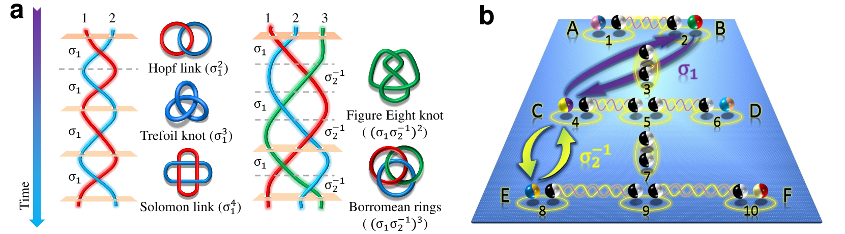
In this study, we calculate Jones polynomial based on the braiding operation of Majorana zero modes. We experimentally simulate the realisation and manipulation of MZMs through our all-optical multi-state interferometers. By employing this photonic quantum simulator that harnesses two-photon correlations and non-dissipative imaginary-time evolution, we implement a sequence of Hamiltonians that induce specific braiding evolutions of MZMs. This approach enables us to perform two distinct braiding operations and apply them to compute the Jones polynomials for five typical links: the Hopf link, Trefoil knot, the Solomon link, Figure Eight knot and Borromean rings [22], as shown in Fig. 1a. The obtained quantum amplitudes demonstrate the topological non-equivalence of these links. Our research demonstrates the feasibility of simulating non-Abelian braiding operations and the subsequent evaluation non-trivial Jones polynomials, setting the stage for further exploration of non-Abelian anyons. Importantly, the topological encoding of quantum information in non-Abelian anyons and its manipulation by braiding them with each other guaranties the highly desired fault-tolerance of the algorithm, throughout its execution. Moreover, it showcases that our photonic quantum simulator, even with its limited scalability, facilitates the experimental realisation of complex topological quantum algorithms.
Results
Majorana-based Jones polynomials. The Jones polynomial of a link , with variable , is related to the quantum amplitude of braided SU(2)k anyons by
| (1) |
where , determines the type of employed anyons, is the quantum dimension of the anyons and is the writhe of the link . State and describe to vacuum anyonic pair creation and annihilation, respectively. We denote by the pair creation of pairs of anyons from the vacuum. The unitary describes the braiding evolution involving one anyon from each pair. The amplitude corresponds to the Markov trace of the braiding operations [23] that span the link with the anyonic worldlines, as shown in Fig. 1a [24].
Strictly speaking the MZMs are not described by a Chern-Simons gauge theory. Nevertheless, the elementary braiding evolutions of Majorana fermions differ from those of SU(2)2 anyons by an overall constant phase factor and they both have quantum dimension . Hence, we can mathematically relate the expectation values, , of arbitrary Majorana evolutions with the Jones polynomial corresponding to the Chern-Simons theory with , in the following way: , where with and the number of anti-clockwise and clockwise exchanges of the link , respectively, and describes the Majorana braiding evolutions that span the link with their worldlines. For the links considered here obtained from the Markov trace of braiding evolutions we always have , resulting in the simple expression
| (2) |
Note that in the conventional algorithm given in [24], Hadamard test is required to measure the amplitude, i.e. the and . However, for the SU(2)2 anyons the Jones polynomial is always a real number (see Supplemental Material for the details). Moreover, to simplify the complexity of our photonic experiment we restrict to the calculation of , which gives us the value of the Jones polynomial up to an overall sign. While this reduces the predictive power of the Jones polynomials, our experiment can still distinguish between several of the targeted links, as we shall see in the following.
We want to realise a set of braiding operations that correspond to a wide family of knots and links, while they are still feasible to implement with our photonic simulator. For that we consider three pairs of Majorana zero modes positioned at the endpoints of three Kitaev chains [25]. Moreover, we choose the size of the chains to be large enough so MZMs are never brought on the same site during the braiding evolution, which would expose the topologically encoded information to local potentials. To achieve fault-tolerance against local potentials at all times during the performance of our algorithm we employ ten fermion sites, as shown in Fig. 1b. Each Tai Chi-like dual-colored sphere represents a Majorana fermion, and two adjacent spheres together constitute a normal fermion. Here, canonical operators and can be used for describing these fermions, with position =1,…,10. The first chain is composed of =1, 2; the second chain is composed of =4, 5, 6 and the third chain is composed of =8, 9, 10. Sites =3 and =7 corresponds to the connections between chains that facilitate the braiding. The Hamiltonian of the initial state in the Kitaev chains can be written as
| (3) |
where and . The Majorana operators satisfies the relations and for . Operators , , , , and are not in the initial Hamiltonian , thus for . Hence, these Majorana modes have zero energy, corresponding to six endpoint MZMs, denoted from A to F in Fig. 1b.
After completing the two sequences of Hamiltonians of braiding operation and (see Methods for the details), the theoretically resulting braiding evolutions in the logical basis are given by and . In (), the last (first) is introduced due to the chain that is not involved in the braiding. According to (2) we can now utilize the combination of the braiding operations and to realise the braiding matrix that corresponds to the desired knots and links shown in Fig. 1a.
Encoding the quantum states based on MZMs. To experimentally implementing the braiding evolution of MZMs, it is necessary to firstly convert the fermionic Hamiltonians into spin Hamiltonians using the Jordan-Wigner (JW) transformation [26]. The resulting spin system exhibits an equivalent spectrum to the original fermion system along the braiding evolution, giving rise to the same non-Abelian Berry phases in their corresponding basis of eigenstates [15]. This enables the simulation of a fermion superconducting system in terms of spin-like degrees of freedom that can be directly encoded in our photonic platform. Methods provide the transformed spin Hamiltonians.
Next, we encode the initial logical state of the three chains in terms of spin states. For convenience, we express the spin states of the system in terms of the eigenvectors , and of the corresponding Pauli operators , and , with eigenvalues , respectively. Then the transformation is given by: , , , , and . Thus, the initial logical state is represented in terms of spins .
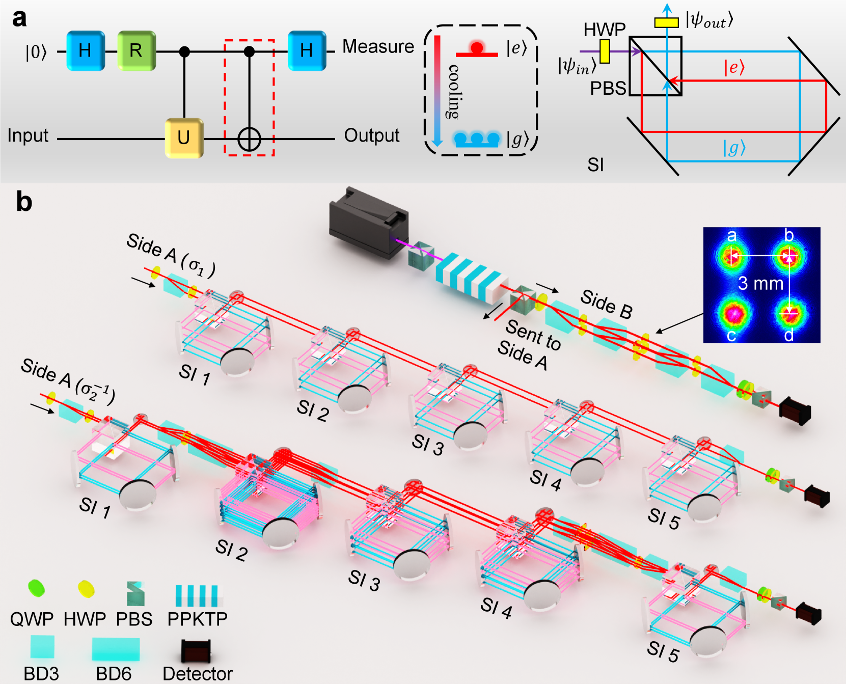
Rather than using single photons to encode the desired spin states we improve the efficiency of our photonic system by employing two-photon correlations [27, 28, 29]. Methods provide the details of two-photon correlations encoding. Fig. 2 shows our experimental setup. A 404 nm continuous wave diode laser is used to pump a type-II periodically poled KTiOPO4 (PPKTP) to generate the two correlated photons through spontaneous parametric down conversion [30]. One of the two photons is sent to side A, and the other photon is sent to side B. On each side, spatial modes of the photon are manipulated via beam displacers (BDs), which are birefringent crystals capable of spatially separating light beams based on their horizontal or vertical polarization. Here, two types of beam displacers are introduced: BD3 with beams separated by 3 mm and BD6 with beams separated by 6 mm. Additionally, half-wave plates (HWPs) and quarter-wave plates (QWPs) are employed to regulate the polarization of the photon, i.e., exchanging the basis between Pauli operators , and .
After completing the initial state preparation, we need to perform the braiding evolution according to their corresponding sequences of Hamiltonians. The braiding can be implemented through a series of imaginary-time evolution (ITE) operators (see Supplemental Material for the details), and the whole process for and can be simplified as and , respectively. Previously [31, 15], we selected an extended evolution time in order to diminish the influence of the high-energy excited states (labeled as ), thereby allowing only the ground states (labeled as ) with the lowest energy to persist following each evolution step.
Here, to avoid the dissipation of the excited states, we design a new scheme inspired by the concept of quantum cooling [32]. The quantum circuit is shown in Fig. 2a. By inserting a control-not (CNOT) gate in the traditional quantum cooling circuit, the non-dissipative ITE is achieved. This can be realised using a designed polarization-dependent Sagnac interferometer (SI). Methods provide the details of the realisation of the CNOT gate. This process emulates quantum cooling by effectively reducing the excited states to their ground states, resulting in zero photon loss during the ITE evolution. The ratio of reflected to transmitted vertical polarization photons exceeds 500:1, ensuring the accuracy of the non-dissipative ITE evolution. This represents a significant advancement compared to our previous experimental approaches, where approximately half of the photons were discarded in each step of the basis transformation (after steps, the total number of photons will decay to of the initial photon numbers) and thus making it challenging to extend the evolution to multiple steps. This enhancement significantly improves our ability to conduct experiments involving multiple evolutionary steps, thereby facilitating the experimental simulation of complex physical processes.
For braiding operation , to realise the non-dissipative evolution according to its spin Hamiltonians, we built five cascaded SIs on side A while keeping the device on side B stationary. For , due to the more complex Hamiltonians, multiple BD3 and BD6 were used alongside the cascaded SIs on side A, which is more experimentally challenging compared with . (The experimental details for these two evolutions can be found in Supplemental Material).
Upon completion of the specific evolution operation, we need to reconstruct the quantum states during the evolution thus ensuring the effectiveness. The states have basis from to , which corresponds to a three-qubit quantum state. We thus project the final state to 64-measurement basis composed of to reconstruct the density matrix of the quantum state such as according to the standard three-qubit quantum state tomography [33].
Specifically, it requires combining the beams from sides A/B into a single beam.
This process involves the use of BDs and HWPs to recombine all the equal-optical path spatial modes on both sides, thus transforming the spatial modes encoded information to polarization information. The relative phase between different states in the interferometer is adjusted by inserting multiple fused silica plates (4×20×0.15 mm, with reflectivity less than 0.2%, not depicted in Fig. 2). The analysis of the polarization information is accomplished through the combination of a QWP, an HWP, and a polarization beam splitter (PBS). (More experimental details for implementing quantum state tomography can be found in Supplemental Material).
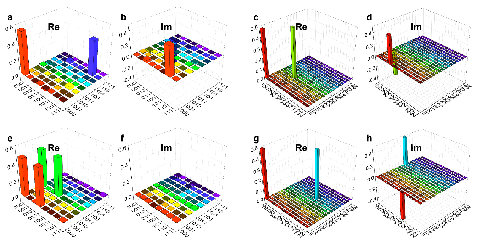
Realisation of braiding operations. We now demonstrate that our experimental setup can faithfully realise the desired braiding evolutions of MZMs. For braiding operation , we perform quantum state tomography on the final state that undergoes the corresponding Hamiltonian transformations. Theoretically, the braiding process transforms the logical Hilbert space with the unitary operation . As a result the initial state should evolve to the final state . The experimentally reconstructed density matrix is shown in Fig. 3a (real part) and b (imaginary part). These measurement results show that we can experimentally produce the final quantum state, , successfully, with a fidelity of 0.992 0.001. We also perform quantum state tomography for all the eigenstates of the Hamiltonians during the braiding process. The average fidelity of these states is 0.991 0.005, indicating the validity and efficacy of each step during the braiding evolution process.
In addition to the reconstruction of the quantum states, we also perform quantum process tomography [34] to characterize the braiding operation . We employ the experimentally intuitive basis and representing the identity, , and , respectively. During the braiding evolution the third chain does not participate so we only need to present the reconstruction of the operator . The experimental results are presented in Fig. 3c (real part) and d (imaginary part). The process fidelity of braiding operation is 0.983 0.014.
Similarly, for braiding operation , we also characterize its performance according to the same procedure in . After the braiding operation , the initial state evolves to the final state . The experimental results are presented in Fig. 3e (real part) and f (imaginary part) with a fidelity of 0.964 0.028. The average fidelity of the final states according to the Hamiltonians during the braiding evolution is 0.978 0.015. Moreover, the reconstructed process matrix (the first chain does not participate) is shown in Fig. 3g (real part) and h (imaginary part) with a fidelity of 0.980 0.015. The experimental results of the state tomography and process tomography demonstrate that we have realised both braiding operations, and , successfully with high fidelity for each step of the evolution.
In our all-optical platform the imperfections of the experimental results stem from flawed interference, imprecise wave plates and fluctuation in the count of photons. Among these three factors, imperfect interference is the primary reason for the incomplete alignment between the experimental results and theoretical values. During the experimental realisation of the main sources of error are imperfections in the five cascaded Sagnac interferometers on Side A, which are experimentally challenging. Meanwhile, the fidelity of both state and process tomography of have decreased slightly compared to . This is because of the additional multiple beam splitters on side A of the setup required for implementing the evolution. For instance, when we implement the ITE process for evolving the final state corresponding to to the final state corresponding to , operation needs to be applied to the final state of . This basis transformation corresponds to experimentally creating eight beams on side A, and then recombining them to four beams which needs interference processes. This process poses significant experimental challenges, especially when these beams have passed through a Sagnac interferometer before recombining. Despite this technical complexity the fidelity of braiding operation still remains exceptionally high, demonstrating the excellent characteristics of our device and its ability to demonstrate Majorana-based Jones polynomial calculations.
Calculation of the Majorana-based Jones polynomials. The braiding operations and are the building blocks for generating a wide variety of links. We consider five combinations of these two braiding operations that give rise to the Jones polynomials of five topologically distinct links when their expectation value with respect to is evaluated. In particular, we realise for the Hopf link, for the Trefoil knot, for the Solomon link, for the Figure Eight knot and for the Borromean rings, as shown in Figs. 1 and 4. The final states after these operations can be directly computed using the experimentally derived process matrix of and .
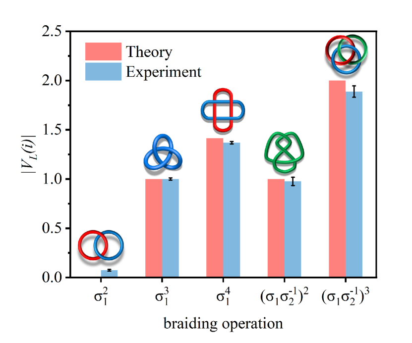
The resulting values of the Jones polynomial for the realised links are shown in Fig. 4. In particular, we obtain that the values of the Jones polynomials for the Hopf link, Trefoil knot, Solomon link, Figure Eight knot and Borromean rings are 0.074 0.008, 1.000 0.011, 1.369 0.013, 0.976 0.042 and 1.888 0.058, respectively. All of these experimentally obtained values match well the theoretical predictions, as shown in Fig. 4. Mathematically, even if the Jones polynomial values of two knots are identical, it does not necessarily mean that they are topologically equivalent [35]. Notably, the Trefoil knot and the Figure Eight knot are topologically distinct despite sharing the same value, . This limitation underscores the difficulty in discerning specific distinct links from their corresponding Jones polynomials when they are evaluated at a specific value [23]. Nevertheless, we can clearly distinguish the links whose values of the Jones polynomials, , are different. Such an advance can greatly contribute in the fields of statistical physics [36], molecular synthesis technology [37] and integrated DNA replication [38], where intricate topological links and knots emerge frequently.
Discussion
In summary, our work utilizes a photonic quantum platform to simulate the braiding operations of Majorana fermions. Two distinct Majorana braiding evolutions are realised that can generate a wide family of topologically distinct links with their worldlines. By measuring the quantum amplitudes of these evolutions we determined the Jones polynomials of the links. Even though these polynomials are evaluated at a non-universal value of their parameter we can directly use them to distinguish between most of the links. In particular, we have experimentally determined the Jones polynomials of five representative links, achieving high-fidelity results that align closely with theoretical predictions.
The topological encoding of information with Majorana anyons is equivalent to encoding information in a quantum error correcting code (QECC) [23]. The added value of manipulating this logical information by braiding anyons is that the information remains encoded in the QECC at all times during the performance of the logical gates. This required a minimum size of ten fermionic sites to fault-tolerantly encode the manipulations between three pairs of anyons, as shown in Fig. 1. Hence, the prototype algorithm we performed for evaluating Jones polynomials is encoded in a QECC that protects it against local errors acting on the fermionic sites at all times. We leave the demonstration of fault-tolerance of our encoded quantum algorithm to a future investigation [15]. The versatility of our platform enables the simulation of a broader range of links, paving the way for the implementation of scalable quantum computation based on fault-tolerant Majorana fermions in various platforms, including superconducting circuits [39], integrated silicon chips [40], and Rydberg atoms [41].
Methods
Hamiltonians during braiding opearion and
We use two basic Majorana braiding operations, and , to generate various knots and links. The first one, , corresponds to the clockwise braiding of MZMs B and C, as shown in Fig. 1b. This evolution is achieved with the following sequence of , , , and back to at last, where
| (4) |
The anticlockwise braiding of C and E implements braiding operation , as shown in Fig. 1b. Its corresponding evolution is achieved with the following sequence: , , , , , and , where
| (5) |
After the Jordan-Wigner (JW) transformation, the superconducting Hamiltonians employed for realising the braiding operation are transformed to spin Hamiltonians
| (6) |
For braiding operation , the superconducting Hamiltonians in (5) are transformed to the spin Hamiltonians
| (7) |
It is worth mentioning that in when evolving from the final state of to that of , we simultaneously change the basis vectors of three Majorana fermions in one step due to the existence of . Such intricate multi-vector transformation is absent in . (The specific ground states of the Hamiltonians in Eqs (6) and (7) can be found in Supplemental Material.)
Two-photon correlation encoding
In Fig. 2, the obtained spatial modes on side A and side B are denoted as and , respectively, where and .
The experiment employs two types of BDs, namely BD3 and BD6, which can spatially separate light beams by 3.0 mm and 6.0 mm, respectively. The coincidence of the spatial modes between the two photons encodes a specific spin bit. Specifically, the two-photon correlation modes are expressed as . For instance, the coincidence between and is regarded as the first term of the state , i.e., , while the rest of the terms of are encoded similarly. The spatial patterns and corresponding encoding relationships of the initial state are summarized in Table I (unnormalized). The subsequent encodings of all states during the evolution exhibit similar characteristics.
Realisation of the CNOT gate
In the Sagnac interferometer (as shown in Fig. 2a), the incoming photon’s horizontal and vertical polarization components are considered as the control qubit and will be equally rotated by an HWP, resulting in . Subsequently, the photon will be split into two paths by a PBS, which transmits the horizontal component and reflects vertical component. Thus, the photons with horizontal polarization propagate in a clockwise direction (blue path) are denoted as the ground state , and the photons with vertical polarization propagate in a counterclockwise direction (red path) are denoted as the excited state , Consequently, the input state can be expressed as . Next, the CNOT gate executes the operation: when the control bit is , the target bit remains unchanged; when the control bit is , the target bit flips, and thus the state becomes . This process corresponds to the emission of the photon’s horizontal and vertical polarization components exiting from the same port of the PBS.
Finally, after the second Hadamard operation (which is realised through an HWP at 22.5°) on the control qubit, the state becomes .
Acknowledgements
This work was supported by the Innovation Program for Quantum Science and Technology (Grants
No. 2021ZD0301200 and No. 2021ZD0301400), the National Natural Science Foundation of China (Grants No. 61975195, No. 11821404, No. 92365205, No. 12374336 and No. 11874343), the Anhui Initiative in Quantum Information Technologies (Grant No. AHY060300) and USTC Research Funds of
the Double First-Class Initiative (Grant No. YD2030002024). J.K.P would like to thank Iason Sofos and Matthew Yusuf for inspiring conversations. J.K.P acknowledges support by EPSRC, Grant No. EP/R020612/1.
Author contributions
Y.-J.H. proposed this project. K.S. designed the experiment. J.-K.L. carried out the
experiment and analysed the experimental results assisted by K.S., Z.-Y.H. and J.-H.L.. J.K.P contributed to the theoretical analysis assisted by S.-J.T.. J.-K.L. and J.K.P wrote the manuscript. J.-S.X., Y.-J.H., C.-F.L. and G.-C.G. supervised the project.
All the authors discussed the experimental procedures and results.
Competing interests
The authors declare no competing interests.
References
- Alexander [1928] J. W. Alexander, Topological invariants of knots and links, Transactions of the American Mathematical Society 30, 275 (1928).
- Kanenobu [1986] T. Kanenobu, Examples on polynomial invariants of knots and links, Mathematische Annalen 275, 555 (1986).
- Kauffman and Lins [1994] L. H. Kauffman and S. L. Lins, Temperley-Lieb Recoupling Theory and Invariants of 3-Manifolds (AM-134) (Princeton University Press, 1994).
- Jones [1985] V. F. R. Jones, A polynomial invariant for knots via von Neumann algebras, Bulletin (New Series) of the American Mathematical Society 12, 103 (1985).
- Podtelezhnikov et al. [1999] A. A. Podtelezhnikov, N. R. Cozzarelli, and A. V. Vologodskii, Equilibrium distributions of topological states in circular dna: Interplay of supercoiling and knotting, Proceedings of the National Academy of Sciences 96, 12974 (1999).
- Taylor [2000] W. R. Taylor, A deeply knotted protein structure and how it might fold, Nature 406, 916 (2000).
- Proment et al. [2012] D. Proment, M. Onorato, and C. F. Barenghi, Vortex knots in a bose-einstein condensate, Phys. Rev. E 85, 036306 (2012).
- Yang et al. [2020] Z. Yang, C.-K. Chiu, C. Fang, and J. Hu, Jones polynomial and knot transitions in hermitian and non-hermitian topological semimetals, Phys. Rev. Lett. 124, 186402 (2020).
- Kuperberg [2009] G. Kuperberg, How hard is it to approximate the jones polynomial?, Theory Comput. 11, 183 (2009).
- Leinaas and Myrheim [1977] J. M. Leinaas and J. Myrheim, On the theory of identical particles, Il Nuovo Cimento B (1971-1996) 37, 1 (1977).
- Wilczek [1982] F. Wilczek, Quantum mechanics of fractional-spin particles, Phys. Rev. Lett. 49, 957 (1982).
- Nayak et al. [2008] C. Nayak, S. H. Simon, A. Stern, M. Freedman, and S. Das Sarma, Non-abelian anyons and topological quantum computation, Rev. Mod. Phys. 80, 1083 (2008).
- Bartolomei et al. [2020] H. Bartolomei, M. Kumar, R. Bisognin, A. Marguerite, J.-M. Berroir, E. Bocquillon, B. Plaçais, A. Cavanna, Q. Dong, U. Gennser, Y. Jin, and G. Fève, Fractional statistics in anyon collisions, Science 368, 173 (2020).
- Witten [1989] E. Witten, Quantum field theory and the jones polynomial, Commun. Math. Phys. 121, 351 (1989).
- Xu et al. [2018] J.-S. Xu, K. Sun, J. K. Pachos, Y.-J. Han, C.-F. Li, and G.-C. Guo, Photonic implementation of majorana-based berry phases, Science Advances 4, eaat6533 (2018).
- Moore and Read [1991] G. W. Moore and N. Read, Nonabelions in the fractional quantum hall effect, Nuclear Physics 360, 362 (1991).
- Sau et al. [2010] J. D. Sau, R. M. Lutchyn, S. Tewari, and S. Das Sarma, Generic new platform for topological quantum computation using semiconductor heterostructures, Phys. Rev. Lett. 104, 040502 (2010).
- Abdumalikov Jr et al. [2013] A. A. Abdumalikov Jr, J. M. Fink, K. Juliusson, M. Pechal, S. Berger, A. Wallraff, and S. Filipp, Experimental realization of non-abelian non-adiabatic geometric gates, Nature 496, 482 (2013).
- Kitaev [2003] A. Y. Kitaev, Fault-tolerant quantum computation by anyons, Ann. Physics 303, 2 (2003).
- Tewari et al. [2007] S. Tewari, S. Das Sarma, C. Nayak, C. Zhang, and P. Zoller, Quantum computation using vortices and majorana zero modes of a superfluid of fermionic cold atoms, Phys. Rev. Lett. 98, 010506 (2007).
- Zhu et al. [2020] S. Zhu, L. Kong, L. Cao, H. Chen, M. Papaj, S. Du, Y. Xing, W. Liu, D. Wang, C. Shen, F. Yang, J. Schneeloch, R. Zhong, G. Gu, L. Fu, Y.-Y. Zhang, H. Ding, and H.-J. Gao, Nearly quantized conductance plateau of vortex zero mode in an iron-based superconductor, Science 367, 189 (2020).
- Alexander and Briggs [1926] J. W. Alexander and G. B. Briggs, On types of knotted curves, Annals of Mathematics 28, 562 (1926).
- Pachos [2012] J. K. Pachos, Introduction to Topological Quantum Computation (Cambridge University Press, 2012).
- Aharonov et al. [2009] D. Aharonov, V. Jones, and Z. Landau, A polynomial quantum algorithm for approximating the jones polynomial, Algorithmica 55, 395 (2009).
- Kitaev [2001] A. Y. Kitaev, Unpaired majorana fermions in quantum wires, Physics-Uspekhi 44, 131 (2001).
- Jordan and Wigner [1928] P. Jordan and E. Wigner, Über das paulische Äquivalenzverbot, Zeitschrift für Physik 47, 631 (1928).
- Ekert [1991] A. K. Ekert, Quantum cryptography based on bell’s theorem, Phys. Rev. Lett. 67, 661 (1991).
- Peruzzo et al. [2010] A. Peruzzo, M. Lobino, J. C. F. Matthews, N. Matsuda, A. Politi, K. Poulios, X.-Q. Zhou, Y. Lahini, N. Ismail, K. Wörhoff, Y. Bromberg, Y. Silberberg, M. G. Thompson, and J. L. OBrien, Quantum walks of correlated photons, Science 329, 1500 (2010).
- Horodecki et al. [2009] R. Horodecki, P. Horodecki, M. Horodecki, and K. Horodecki, Quantum entanglement, Rev. Mod. Phys. 81, 865 (2009).
- Eisaman et al. [2011] M. D. Eisaman, J. Fan, A. L. Migdall, and S. V. Polyakov, Invited review article: Single-photon sources and detectors., The Review of scientific instruments 82 7, 071101 (2011).
- Xu et al. [2016] J.-S. Xu, K. Sun, Y.-J. Han, C.-F. Li, J. K. Pachos, and G.-C. Guo, Simulating the exchange of majorana zero modes with a photonic system, Nature Communications 7, 13194 (2016).
- Xu et al. [2014] J.-S. Xu, M.-H. Yung, X.-Y. Xu, S. Boixo, Z.-W. Zhou, C.-F. Li, A. Aspuru-Guzik, and G.-C. Guo, Demon-like algorithmic quantum cooling and its realization with quantum optics, Nature Photonics 8, 113 (2014).
- Leonhardt [1995] U. Leonhardt, Quantum-state tomography and discrete wigner function, Phys. Rev. Lett. 74, 4101 (1995).
- O’Brien et al. [2004] J. L. O’Brien, G. J. Pryde, A. Gilchrist, D. F. V. James, N. K. Langford, T. C. Ralph, and A. G. White, Quantum process tomography of a controlled-not gate, Phys. Rev. Lett. 93, 080502 (2004).
- Kauffman [2001] L. H. Kauffman, Knots and Physics, 3rd ed. (WORLD SCIENTIFIC, 2001) https://worldscientific.com/doi/pdf/10.1142/4256 .
- Zhou et al. [2021] J.-R. Zhou, Q.-R. Wang, C. Wang, and Z.-C. Gu, Non-abelian three-loop braiding statistics for 3d fermionic topological phases, Nature Communications 12, 3191 (2021).
- Guo et al. [2010] J. Guo, P. C. Mayers, G. A. Breault, and C. A. Hunter, Synthesis of a molecular trefoil knot by folding and closing on an octahedral coordination template, Nature Chemistry 2, 218 (2010).
- Liu et al. [2016] D. Liu, G. Chen, U. Akhter, T. M. Cronin, and Y. Weizmann, Creating complex molecular topologies by configuring dna four-way junctions, Nature Chemistry 8, 907 (2016).
- Khazali and Mølmer [2020] M. Khazali and K. Mølmer, Fast multiqubit gates by adiabatic evolution in interacting excited-state manifolds of rydberg atoms and superconducting circuits, Phys. Rev. X 10, 021054 (2020).
- Zhao et al. [2020] Y. Zhao, Y. Okawachi, J. K. Jang, X. Ji, M. Lipson, and A. L. Gaeta, Near-degenerate quadrature-squeezed vacuum generation on a silicon-nitride chip, Phys. Rev. Lett. 124, 193601 (2020).
- González-Cuadra et al. [2022] D. González-Cuadra, T. V. Zache, J. Carrasco, B. Kraus, and P. Zoller, Hardware efficient quantum simulation of non-abelian gauge theories with qudits on rydberg platforms, Phys. Rev. Lett. 129, 160501 (2022).