Photonic Matrix Multiplier Makes a Direction-Finding Sensor

Direction finding is a pivotal technology for identifying or determining the direction from which a received signal at radio or microwave frequencies originates. This practice is extensively used in a plethora of applications, including radar, wireless communications, and radio astronomy. The essential process involves the use of a radio receiver and antenna system to determine the spatial direction of an incoming radio signal. There are numerous methods applied for direction finding at RF and microwave frequencies [1, 2], such as amplitude and phase comparison monopulse [3, 4, 5], sequential lobing [6, 7] (conical scanning and nutating), frequency interferometry [8], and time difference of arrival [9, 10, 11, 12]. In the optical frequency range, methods for direction finding often fall under the category of optical beamforming or beam steering, which is widely utilized in lidar (light detection and ranging) systems [13, 14, 15, 16, 17], free-space optical communications [18], and various other applications [19]. In recent years, with the progress in developing densely packed photonic integrated circuits, numerous approaches have been undertaken to develop on-chip photonic lidar [20, 21, 22] and remote sensing systems [23, 24].

In the past decade, there has been significant progress in developing programmable photonic integrated circuits capable of performing arbitrary discrete linear operations. This includes solutions based on meshes of Mach-Zehnder interferometers (MZI) [25, 26, 27], multimode interference (MMI) couplers [28], and multiport waveguide arrays [29, 30, 31, 32, 33, 34, 35]. The latter has been possible on platforms based on silicon solutions, such as SiO2 and SiN, where a high contrast refractive index is generated, rendering strongly confined and low-disperse guide modes propagating through waveguides [36]. In turn, tunable phase shifters based on thermo-optical [37] and phase-change materials [38] (PCM) are implemented to program the device for the desired functionality. Given the scalability of these photonic circuits, programmable photonics has become an emerging and attractive technology that holds great promise for numerous applications in classical [39] and quantum information processing [40, 41]. Despite the rapid development of programmable photonic integrated circuits, it remains to fully exploit novel functionalities for various use cases. Recent efforts have been put to deploy optical convolutional layers [42, 43], neuromorphic optical computing [44, 45], and high-speed communication channels [46, 47].

In this work, we aim to focus on the direction-of-arrival finding and investigate the possibility of performing this fundamental task through a photonic matrix-vector multiplier circuit. We derive the required conditions and fundamental limitations so that a photonic circuit architecture for on-chip direction finding can be devised. The proposed architecture, shown schematically in Fig. 1, is based on a linear and equally spaced array of $M$ grating couplers that sample the phasefront of incoming plane waves. This discrete $M$-dimensional vector $\mathbf{x}\in\mathbb{C}^{M}$ is then steered into a photonic matrix-vector multiplier device that maps the phase slope of the incoming wave onto a localized intensity vector $\mathbf{y}\in\mathbb{C}^{N}$ at $N$ output ports. We consider and explore the general scenario in which the number of input ($M$) and output ports ($N$) is different. Thus, the photonic unit is, in general, non-unitary and is devised by imposing transformation rules on a set of incident sampling angles. This allows the transfer matrix of the device to be uniquely defined based on the design parameters, such as the number of grating couplers and their separation, as well as the detection aperture angle and the total number of output ports of the photonic processing unit. The detection functionalities of the device are proven to be continuously extended beyond the discrete sampling angles by introducing suitable tracking functions implemented in a post-processing stage at the output of the core photonic processor. The fundamental limits of each tracking function are discussed through pertinent examples. Lastly, an approximation is discussed so that the photonic operation reduces to a unitary one, rendering a compact device at the expense of compromises on the detection capabilities.

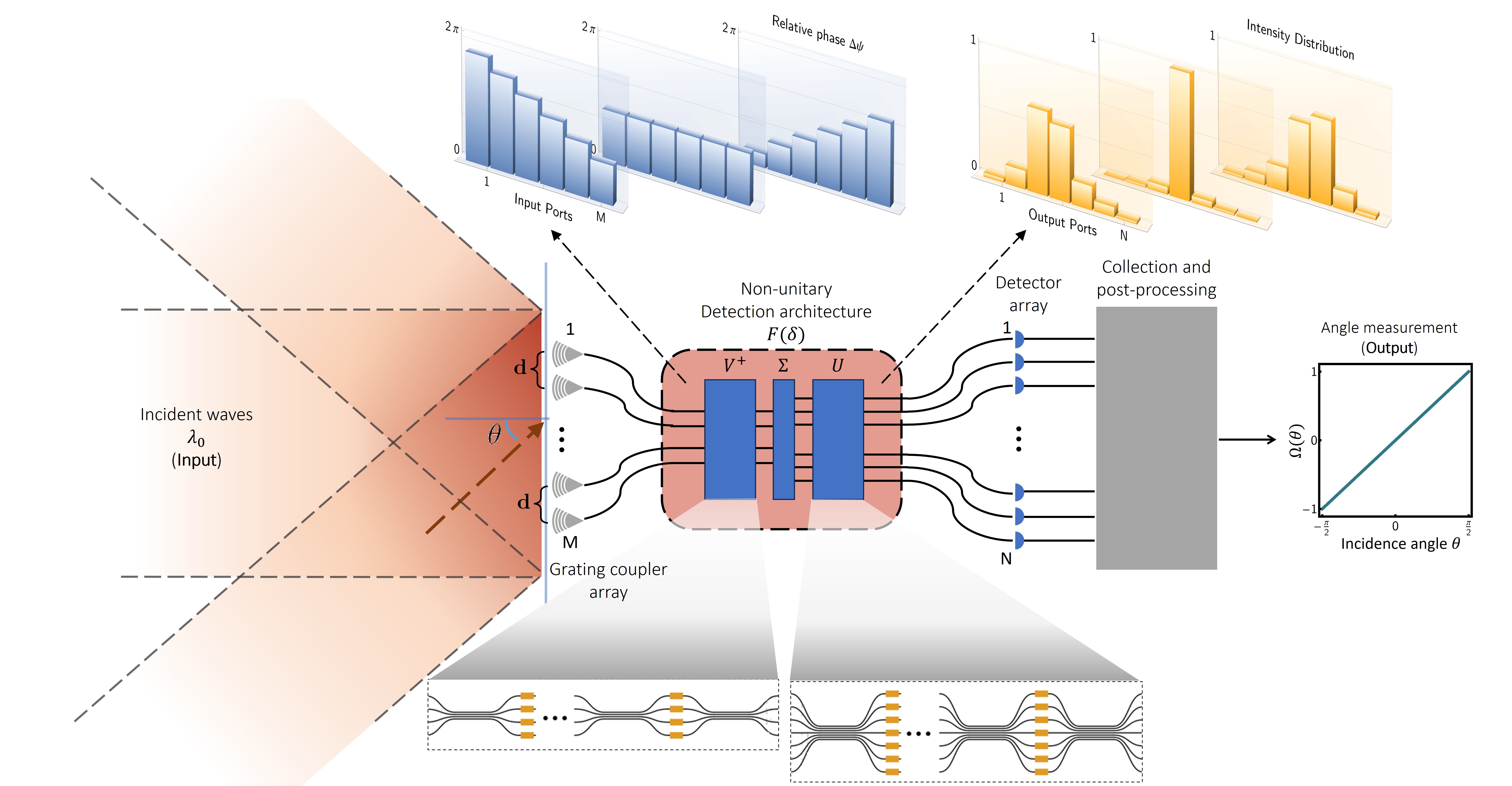
Let us consider an incoming plane wave with wavenumber $k_{0}$ traveling in the direction $\hat{\mathbf{r}}$. The wavefront is assumed to be incident onto an equally spaced linear array of $M$ grating couplers that take discrete samples of the plane wave. The distance between contiguous grating couplers is denoted by $d$, and the wavevector of the incoming plane wave makes an angle $\theta$ with respect to the linear array. These grating couplers collect the plane waves and steer them to a still unknown linear optical processor with transfer matrix $F$ that pre-processes the light gathered at the grating couplers and produces an $N$-port output $\mathbf{y}\in\mathbb{C}^{N}$, which is meant to be further processed to extract the features of the incident angle. The proposed architecture is sketched in Fig. 1. The optical processor is characterized by the linear operator $F\in\mathbb{C}^{N\times M}$, the explicit form of which is determined based on the input and output relations imposed on the system.

We define the incident wave at a particular granting coupler as $e^{i\xi}/\sqrt{M}$, where the factor $1/\sqrt{M}$ is considered for normalization. Thus, straightforward calculations show that the contiguous grating coupler shall collect the wave $e^{i(\xi\pm k_{0}d\sin\theta)}/\sqrt{M}$. In this form, a vector $\mathbf{x}(\theta)$ containing the electric fields as measured at each of the $M$ spots on the grating coupler array, up to a global phase, is given by

$$\mathbf{x}(\theta)=\frac{1}{\sqrt{M}}\left(e^{-i\psi(\theta)},e^{-2i\psi(\theta)},\ldots,e^{-Mi\psi(\theta)}\right)^{T},$$

(1)

where, $\psi(\theta):=k_{0}d\sin\theta$, with $\theta\in(-\pi/2,\pi/2)$, while $(\cdot)^{T}$ denotes the matrix transpose operation, and the factor $1/\sqrt{M}$ is for normalization.

The first stage of the device is then characterized by the set of linear operations $\mathbf{y}_{n}=F\mathbf{x}_{n}$, with $n=1,2,\ldots,N$ and $\mathbf{x}_{n}\in\mathbb{C}^{M}$ and $\mathbf{y}_{n}\in\mathbb{C}^{N}$ the respective input and output vectors of the transformation to be defined.

Here, we focus on a direction-finding device that, for a specific set of wavefronts with discrete incident angles $\{\theta_{n}\}_{n=1}^{N}$, produces a single impulse at the $n$-th output port of the photonic processor. Note that the number of sampling angles $\theta_{n}$ and the number of output ports is $N$, which is, in general, different from the number of grating couplers $M$. The previous requirements allow for the construction of a simple device that requires low computational power and performs a discrete detection operation, while we later discuss that the angle detection can be readily generalized to cover a continuous range. Since the grating couplers are linearly arranged, the maximum detection range (aperture angle) is $\pi$. For symmetry reasons, we choose the following discrete set of incident sampling angles:

$$\theta_{n}(\delta):=\left(-\frac{\pi}{2}+\delta\right)\left(\frac{N-2n+1}{N-1}\right),\quad n\in\{1,\ldots,N\}.$$

(2)

These angles are uniformly distributed in the interval $(-\pi/2+\delta,\pi/2-\delta)$, where $\delta$ controls the aperture angle for the detection scheme. Since we want to steer a specific incident wave with angle $\theta_{n}$ to the $n$-th output port, the direction-finding optical processor $F\equiv F(\delta)$ is devised through reverse engineering by imposing the set of input and output relations of the form

$$\hat{\mathbf{e}}_{n}=F(\delta)\mathbf{x}_{n}(\delta),\quad n\in\{1,\ldots,N\},$$

(3)

where we have defined the set of discrete sampling vectors

$$\mathbf{x}_{n}(\delta):=\mathbf{x}\left(\theta=\theta_{n}(\delta)\right),\quad n\in\{1,\ldots,N\},$$

(4)

with $\hat{\mathbf{e}}_{n}=(0,\ldots,1,\ldots,0)^{T}$ the $n$-th vector of the canonical basis and $\mathbf{x}(\theta)$ is given in (1). To extract a simpler relation for $F(\theta)$, we exploit the fact that $\{\hat{\mathbf{e}}_{n}\}_{n=1}^{N}$ forms an orthonormal basis in $\mathbb{C}^{N}$. We thus multiply (3) by $\hat{\mathbf{e}}_{n}^{\dagger}$ to the right and sum over $n$ to render the relation

$$\mathbb{I}_{N}=F(\delta)G(\delta),\quad G(\delta):=\sum_{n=1}^{N}\mathbf{x}_{n}\hat{\mathbf{e}}_{n}^{\dagger}\equiv\left(\mathbf{x}_{1}(\delta),\ldots,\mathbf{x}_{N}(\delta)\right).$$

(5)

where $\mathbb{I}_{N}$ is the identity matrix in $\mathbb{C}^{N\times N}$ and $G(\delta)\in\mathbb{C}^{M\times N}$. Nevertheless, the exact form and solvability of $F(\delta)$ is constrained to the exact relation between the number of output ports ($N$) and grating couplers ($M$).

For $M=N$, $G(\delta)$ reduces to a non-unitary square matrix. The non-unitarity becomes evident as the column vectors $\mathbf{x}_{n}$ are not orthonormal. However, the invertibility is ensured as $G(\delta)$ takes the form of a non-uniform discrete Fourier transform [48] (NUDFT), alternatively known as Vondermonde matrices [49, 50]. From this, the existence and uniqueness of the inverse of $G(\delta)$ is secured since the determinant of Vondermonde matrices [49] is always non-null. Thus, $F(\delta)$ always exists for $N=M$, and our construction ensures that the output will exactly reproduce an excitation in one single output port for plane waves incident at the exact angle $\theta_{n}$.

In turn, for $M\neq N$, the transforms $F$ and $G$ are defined by rectangular matrices whose inverses either do not exist or are not uniquely defined. This issue is overcome by considering the pseudo-inverse, also known as the Moore-Penrose inverse [51], denoted by $G^{-}$. The latter fulfills the property $GG^{-}G=G$, which holds for square nonsingular matrices, as well as for left-inverse and right-inverse matrices for rectangular matrices. Note that Eq. (5) defines a system of $N^{2}$ equations and $NM$ unknown variables $F_{p,q}$, which leads to an over-parameterized and an under-parameterized problem form $M<N$ and $M>N$, respectively. The former has more than one solution, whereas the latter does not have a solution. Here, the pseudo-inverse $G^{-}$ allows for a solution (5), for its existence and uniqueness are ensured and can be determined from the singular value decomposition (SVD) of the matrix in question. That is, $G=U\Sigma V^{\dagger}$, with $U$ and $V$ unitary matrices and $\Sigma$ a diagonal matrix containing the singular values of $G$. For $M<N$, $G^{-}$ provides a particular exact solution. For $M>N$, $G^{-}$ yields the best approximate solution that minimizes the involved least square problem [52]. Therefore, in all cases, the liner operator characterizing the device is

$$F(\delta)=G^{-}(\delta),\quad G^{-}(\delta)=V\Sigma^{-}U^{\dagger},$$

(6)

where $U$ and $V$ are computed from the SVD of $G(\delta)$, and $\Sigma^{-}$ is the pseudo-inverse of $\Sigma$. To illustrate the two cases posed above, we illustrate in Fig. 2 the out output mode $\mathbf{y}_{n}=F\mathbf{x}_{n}$ for $N=7$ and $M=4,10$, and grating couplers separation in the sub-wavelength domain $d_{0}=\lambda_{0}/2\pi$. In such a case, the output renders the desired operation $\mathbf{y}_{n}=\hat{\mathbf{e}}_{n}$ for $M>N$, as expected. In turn, one might notice a distribution for $M<N$ whose peak is located at the $n$-th port. This solution is the best approximation for the under-parameterized set of equations, which still captures part of the direction-finding operation. Lastly, for $M=N$, the pseudo-inverse reduces to the conventional inverse discussed above.

The operator $F(\delta)$ has been constructed so that the set of discrete incident angles $\mathbf{x}_{n}$ can be exactly detected at the output. However, incident waves at the grating couplers arrive at continuous angles. Thus, to keep a better track of the incident wave angle, a post-processing operation on the signal generated by $F(\delta)$ is required so that the detection capabilities of the device extend beyond the $N$ incident angles $\mathbf{x}_{n}$. To this end, it is convenient to inspect $F(\delta)\mathbf{x}(\theta)$ for a continuum interval $\theta\in(-\pi/2+\delta,\pi/2-\delta)$. Such an operation is portrayed in Fig. 3 for $N=7$ and a grating coupler separation $d=\lambda_{0}\ell=1$, with $\ell=1/2\pi$, and the three possible cases $M=4,7,10$. From the latter, one may note that the intensity distribution has a maximum whose location moves from the first output port ($n=1$) to the last one ($n=N=7$). Additionally, for a fixed $\theta$, the output distribution has small tails around such the maximum, resembling the shape of a probability distribution. The latter is not necessarily normalized as $F(\delta)$ defines a non-unitary transform, even for $M=N$. Likewise, a similar behavior is found for $M>N$, where the pseudo-inverse $G^{-}$ is exact. Although the distribution spreads more for $M<N$, where the pseudo-inverse is only approximated, the overall dynamic is similar to the other cases.

The latter suggests that some aperture detection angles can be detected by either analyzing the intensity distribution across the output ports or pre-processing it before its detection. One way to achieve continuous tracking of the incident wave angle $\theta$ is by defining the position vector $\mathbf{q}:=(1,\ldots,N)^{T}$ and computing the “average position” defined through the matrix-vector multiplication

$$\Omega(\theta;\ell):=|\mathbf{q}^{\dagger}F(\delta;\ell)\mathbf{x}(\theta)|,\quad\mathbf{q}=(1,2,\ldots,N)^{T},\quad d=\ell\lambda_{0},$$

(7)

with $\mathbf{q}^{\dagger}$ the complex transpose (adjoint) of $\mathbf{q}$. In the latter, we have rescaled the grating coupler spacing in terms of the incident wavelength $\lambda_{0}=2\pi/\kappa_{0}$ through the relation $d=\ell\lambda_{0}$, where $\ell$ defines the spacing factor. From now on, we refer to $\Omega(\theta;\ell)$ as the continuous tracking measure. Remark that incident angles in the set $\theta\in\{\theta_{n}\}_{n=1}^{N}$ yield to $\Omega(\theta_{n};\ell)=n$; i.e., the continuous tracking measure leaves invariant the original detection angles scheme of the sampling angles $\mathbf{x}_{n}$. To make a reliable prediction of the incident angle out of the continuous tracking function, the $\Omega(\theta;\ell)$ shall define a one-to-one function so that no ambiguity exists in the output measurement with respect to the incident angle $\theta\in(-\pi/2+\delta,\pi/2-\delta)$ for a fixed grating coupler separation $d=\lambda_{0}\ell$. Otherwise, the angle detection would be ambiguous and thus ill-defined.

Alternatively, a second measure can be established to track the incident wave angle. As pointed out above, the maximum of the intensity distribution $|F(\delta;\ell)\mathbf{x}(\theta)|$ moves in discrete steps along the incident angle $\theta$. This suggests an alternative operation of the form

$$\Phi(\theta;\ell)=max(|F(\delta;\ell)\mathbf{x}(\theta)|),$$

(8)

where $max(|\mathbf{z}|)$ computes the position $n\in\{1,\ldots,N\}$ in which the maximum element $|z_{n}|$ of $|\mathbf{z}|$ is located. Clearly, this measure defines a discrete mapping $\Phi(\theta;\ell):\mathbb{C}^{N}\mapsto\mathbb{N}$, which also preserves the output for the sampling discrete angles $\{\theta_{n}\}_{n}^{N}$; that is, $\Phi(\theta_{n};\ell)=n$, just like the continuous tracking measure does. Henceforth, we refer to $\Phi(\theta;\ell)$ as the discrete tracking measure.

Although the device operator $F(\delta)$ can be precisely constructed for any combination of the parameter set $\{\ell,M,N\}$, the continuous and discrete tracking functions might not be suitable for all arbitrary values of such parameters. Some compromises might arise when dealing with different spacing factors $\ell$. To this end, Fig. 4(a)-(b) illustrates the behaviour of the $\Omega(\theta;\ell)$ and $\Phi(\theta;\ell)$ as a function of both the incident wave angle $\theta$ and the spacing factor $\ell$. Here, we focus on $\ell<1$, which defines grating couplers spaced in the sub-wavelength regime and output ports $N=5$ and $N=20$. For $N=7$, the discrete measure works as required for $\ell\in(0.05,0.31)$ regardless of the values of $M$. Despite the latter, the resolution of the measure is relatively poor, as only seven angles can be reported. In turn, the continuous measure can be used indeed, but only for limited cases of the spacing factor $\ell\lessapprox 0.15$. For larger values of $\ell$, $\Omega(\theta;\ell)$ ceases to be a one-to-one function and is thus discarded as a candidate for tracking function. This is portrayed in Fig. 4(c).

The situation improves by increasing the number of output ports to $N=20$, where $\Omega(\theta;\ell)$ becomes a well-posed tracking function for $\ell\lessapprox 0.28$ when $M=20$ and $M=15$, and similarly for $\ell\lessapprox 0.25$ when $M=25$. For clarity, the reliability is further illustrated in Fig. 4 for $\ell=0.15$ and $\ell=0.3$. For $\ell=0.3$ and $N=7$, $\Omega(\theta;\ell)$ shall be ruled out for any $M$ and be replaced by $\Phi(\theta;\ell)$ instead. Likewise, for $\ell=0.3$ and $N=20$, both $\Omega(\theta;\ell)$ and $\Phi(\theta;\ell)$ are suitable except for $M=25$. This provides some guidelines for the design of the final device based on the accuracy and compactness requirements.

The all-optical implementation for the direction finder architecture described by the non-unitary matrix $F(\delta)$ can be determined, in general, by using singular value decomposition (SVD), which in each case is straightforwardly obtained by numerical means. This is done for every configuration, leading to the factorization

$$F=U\Sigma V^{\dagger},$$

(9)

with $U\in\mathbb{C}^{N\times N}$ and $V\in\mathbb{C}^{MM}$ unitary matrices. In turn, $\Sigma\in\mathbb{C}^{M\times N}$ is a semi-positive definite rectangular diagonal matrix.

The factorization (9) makes it possible to design an equivalent photonic circuit that captures all the properties of the direction-finding element. On the one hand, the two unitary elements can be constructed either through meshes of MZI [53, 54, 55] or arrays of coupled waveguides [29, 56, 33]. In turn, the middle section of the architecture $\Sigma$ involves a semi-positive rectangular diagonal matrix, which can be deployed using a $N$-parametric layer of MZI interferometers. Although each MZI requires two-phase elements to steer both amplitude and phase, one MZI is required in the current approach since the architecture involves only amplitude modulation. Alternatively, amplitude modulation is achievable by utilizing phase-change materials (PCM), which allows for a more compact solution as compared to the MZI array [38, 57, 58]. If $\ell$ is a fixed quantity due to the non-tunability of the grating coupler separation, the transmission matrix $F(\delta)$ is also fixed. This permits designing the corresponding photonic circuit so that no active elements are needed. This holds if we use MZI as the modulation layer, whereas for PCMs, there is still a power consumption requirement to operate them. Here, the unitaries $U$ and $V^{\dagger}$ are implemented using interlaced layers of phase shifters $P^{(n)}$ and waveguide arrays $G$ through the universal factorization [33]

		$\displaystyle\mathcal{U}=GP^{(K+1)}G\ldots GP^{(1)}G,$		(10)
		$\displaystyle G=e^{-iHL},\quad P^{(n)}_{p,q}=e^{i\phi_{p}^{(n)}}\delta_{p,q},$

where $L$ is the coupling length of the waveguide array, $\phi^{(n)}_{p}\in(0,2\pi)$ is the p-th phase element in the n-th layer, $p,q\in\{1,\ldots,K\}$ and $K\in\mathbb{Z}^{+}$. Here, $K$ is the dimension of the corresponding target unitary matrix $\mathcal{U}$, which can be either N and M for $U$ and $V^{\dagger}$, respectively. The tridiagonal matrix $H\in\mathbb{R}^{K\times K}$ corresponds to the JX lattice Hamiltonian [59], with components $H_{p,q}=\kappa_{p+1}\delta_{p+1,q}+\kappa_{p}\delta_{p-1,q}$ for $p,q\in\{1,\ldots,K\}$.

Sketches of the photonic circuits related to the architecture $F(\delta)$ are depicted in Fig. 5. The yellow blocks denote the phase elements, and the red blocks are the amplitude modulation elements. Particularly, Figs. 5(a)-(b) show the cases $M<N$ and $M>N$, respectively, where clearly not all ports of the unitary matrices $V^{\dagger}$ and $U$ are connected. This suggests that $F(\delta)$ can be rendered using lesser elements in one of the unitaries. Indeed, the universality of Eq. (10) was numerically shown for $K(K+1)$ phase elements [56, 33]. Here, for $N\neq M$ and from the SVD, one may note that fewer phase elements are required. To illustrate this, recall that $\Sigma$ is a $M\times N$ rectangular diagonal matrix with $(N-M)$ zero columns and $(M-N)$ zero rows for $M<N$ and $M>N$, respectively. This implies that only the first $M$ rows of $V^{\dagger}$ ($M<N$) and $U$ ($N>M$) are meaningful for the reconstruction of $F(\delta)$, and the resulting unitary architectures shall require less optical elements.

In summary, we showed that the direction-of-arrival sensing for optical waves could be formulated as a proper mapping of phase distributions onto amplitude distributions in multiport photonic devices. More importantly, such a mapping can be efficiently performed through a linear matrix operation. This was achieved by the inverse design of a programmable photonic matrix-vector multiplier device structure based on a set of input and output relations. In doing so, there is a degree of arbitrariness in defining the input/output relations. In this work, a simple set of rules was imposed to map a discrete set of plane waves with contiguous equidistant angles onto single-channel intensity peaks in the output. This simple rule straightforwardly leads to the inverse operator required for such a task in the form of a Non-uniform Discrete Fourier Transform (NUDFT), the inverse of which is ensured from the properties of Vondermonde matrices. One of the main drawbacks of this approach lies in the non-unitarity of the final transformation. Despite the latter, the device can be implemented through all-photonic components by decomposing it into its singular value decomposition. This permits the identification of three components, two unitary parts, and an amplitude modulator in the form of a diagonal matrix. Clearly, this prohibits intensity preservation and, thus, the use of active elements to scale up or attenuate the intensity depending on the case under consideration.

The main advantage of our architecture lies in the capacity to perform continuous tracking of the incident plane wave angles, a task possible by analyzing the intensity pattern at the output. This reveals a distribution-like pattern whose peak moves with the incident wave angle, suggesting the existence of a mathematical operation to track such an angle. Although there is no unique way to perform such an operation, it was found that the position average operation allows the desired tracking. For this, it is required that the separation between the arrays of grating couplers remain in the sub-wavelength regime, as for large values, the continuous measure function (7) ceases to define a one-to-one mapping. Nevertheless, in the latter case, one can define a discrete tracking measure, i.e. (8). This becomes a valuable resource when the number of output ports is relatively large, for the accuracy increases with $N$, which was illustrated for $N=7$ and $N=20$.

We showed that the proposed non-unitary photonic processor can be approximated to a unitary by identifying the appropriate separation distance between the grating coupler arrays and for certain detection aperture angles. This is achieved when the non-uniform sampling $\psi(\theta_{q})$ becomes a linear function of the port number $q\in\{1,\ldots,N\}$. However, this compromise generally reduces the capabilities of the device, limiting the detection aperture angle to a maximum interval of $(-\pi/4,\pi/4)$ and making continuous tracking unfeasible beyond a certain grating coupler spacing. Nonetheless, the approximation does not restrict the total number of ports $N$, allowing for improved detection accuracy. Despite the approximation trade-off, the resulting unitary device is reliable within its range of applicability, and its construction requires less than half of the number of components compared to its non-unitary counterpart and, does not require amplitude modulators, thus significantly reducing the overall footprint of the device.

Although the focus of this work is on direction-of-arrival finding, the device concept and theoretical framework presented here can also be applied to the reverse operation, i.e., beam steering. This framework can be generalized for use with programmable photonic circuits to develop photonic integrated circuit LiDAR systems/subsystems. These systems offer greater flexibility compared to conventional designs based on phased arrays (PAs) and focal plane arrays (FPAs). It remains to explore features such as size and weight, power consumption, resolution, and field of view for such programmable photonic LiDAR systems.

\bmsection

Funding This project is supported by the U.S. Air Force Office of Scientific Research (AFOSR) Young Investigator Program (YIP) Award# FA9550-22-1-0189, and the U.S. National Science Foundation (NSF) FuSe grant # 2329021.

\bmsection

Disclosures The authors declare no conflicts of interest.

\bmsection

Data availability Data underlying the results presented in this paper are not publicly available at this time but may be obtained from the authors upon reasonable request.

References

- [1] J. Yao, “Microwave photonics,” \JournalTitleJournal of Lightwave Technology 27, 314–335 (2009).
- [2] D. Pérez-López, A. Gutierrez, D. Sánchez, et al., “General-purpose programmable photonic processor for advanced radiofrequency applications,” \JournalTitleNature Communications 15, 1563 (2024).
- [3] S. M. Sherman and D. K. Barton, Monopulse principles and techniques (Artech House, 2011).
- [4] T. Ito, R. Takahashi, and K. Hirata, “An antenna arrangement for phase comparison monopulse doa estimation using nonuniform planar array,” in 2011 8th European Radar Conference, (IEEE, 2011), pp. 277–280.
- [5] R. Feng, F. Uysal, P. Aubry, and A. Yarovoy, “Mimo–monopulse target localisation for automotive radar,” \JournalTitleIET Radar, Sonar & Navigation 12, 1131–1136 (2018).
- [6] K. Lo, “Theoretical analysis of the sequential lobing technique,” \JournalTitleIEEE Transactions on Aerospace and Electronic Systems 35, 282–293 (1999).
- [7] Ç. Candan and S. Koç, “Direction finding accuracy of sequential lobing under target amplitude fluctuations,” \JournalTitleIET Radar, Sonar & Navigation 9, 92–103 (2015).
- [8] K.-S. Isleif, O. Gerberding, T. S. Schwarze, et al., “Experimental demonstration of deep frequency modulation interferometry,” \JournalTitleOptics Express 24, 1676–1684 (2016).
- [9] B. Vidal, M. Á. Piqueras, and J. Martí, “Direction-of-arrival estimation of broadband microwave signals in phased-array antennas using photonic techniques,” \JournalTitleJournal of lightwave technology 24, 2741 (2006).
- [10] X. Zou, W. Li, W. Pan, et al., “Photonic approach to the measurement of time-difference-of-arrival and angle-of-arrival of a microwave signal,” \JournalTitleOpt. Lett. 37, 755–757 (2012).
- [11] P. Pertilä, M. Parviainen, V. Myllylä, et al., “Time difference of arrival estimation with deep learning–from acoustic simulations to recorded data,” in 2020 IEEE 22nd International Workshop on Multimedia Signal Processing (MMSP), (IEEE, 2020), pp. 1–6.
- [12] X. Zhang, H. Chi, Y. Gao, et al., “Photonic angle-of-arrival measurement of microwave signals using a triangular wave,” \JournalTitleOptics Letters 48, 5013–5016 (2023).
- [13] C. V. Poulton, A. Yaacobi, D. B. Cole, et al., “Coherent solid-state lidar with silicon photonic optical phased arrays,” \JournalTitleOptics letters 42, 4091–4094 (2017).
- [14] K. Shang, C. Qin, Y. Zhang, et al., “Uniform emission, constant wavevector silicon grating surface emitter for beam steering with ultra-sharp instantaneous field-of-view,” \JournalTitleOptics express 25, 19655–19661 (2017).
- [15] X. Zhang, K. Kwon, J. Henriksson, et al., “A large-scale microelectromechanical-systems-based silicon photonics lidar,” \JournalTitleNature 603, 253–258 (2022).
- [16] K. Sayyah, R. Sarkissian, P. Patterson, et al., “Fully integrated fmcw lidar optical engine on a single silicon chip,” \JournalTitleJournal of Lightwave Technology 40, 2763–2772 (2022).
- [17] S. SeyedinNavadeh, M. Milanizadeh, F. Zanetto, et al., “Determining the optimal communication channels of arbitrary optical systems using integrated photonic processors,” \JournalTitleNature Photonics pp. 1–7 (2023).
- [18] C. V. Poulton, D. Vermeulen, E. Hosseini, et al., “Lens-free chip-to-chip free-space laser communication link with a silicon photonics optical phased array,” in Frontiers in Optics, (Optica Publishing Group, 2017), pp. FW5A–3.
- [19] Q. Cheng, M. Bahadori, M. Glick, et al., “Recent advances in optical technologies for data centers: a review,” \JournalTitleOptica 5, 1354–1370 (2018).
- [20] S. Chung, M. Nakai, S. Idres, et al., “19.1 optical phased-array fmcw lidar with on-chip calibration,” in 2021 IEEE International Solid-State Circuits Conference (ISSCC), vol. 64 (IEEE, 2021), pp. 286–288.
- [21] A. Khachaturian, R. Fatemi, A. Darbinian, and A. Hajimiri, “Discretization of annular-ring diffraction pattern for large-scale photonics beamforming,” \JournalTitlePhotonics Research 10, 1177–1186 (2022).
- [22] A. Khachaturian, R. Fatemi, and A. Hajimiri, “Achieving full grating-lobe-free field of view with low-complexity co-prime photonic beamforming transceivers,” \JournalTitlePhotonics Research 10, A66–A73 (2022).
- [23] A. White, P. Khial, F. Salehi, et al., “A silicon photonics computational lensless active-flat-optics imaging system,” \JournalTitleScientific Reports 10, 1689 (2020).
- [24] G. Serafino, S. Maresca, C. Porzi, et al., “Microwave photonics for remote sensing: From basic concepts to high-level functionalities,” \JournalTitleJournal of Lightwave Technology 38, 5339–5355 (2020).
- [25] W. R. Clements, P. C. Humphreys, B. J. Metcalf, et al., “Optimal design for universal multiport interferometers,” \JournalTitleOptica 3, 1460–1465 (2016).
- [26] F. Shokraneh, S. Geoffroy-Gagnon, and O. Liboiron-Ladouceur, “The diamond mesh, a phase-error-and loss-tolerant field-programmable mzi-based optical processor for optical neural networks,” \JournalTitleOptics Express 28, 23495–23508 (2020).
- [27] K. Rahbardar Mojaver, B. Zhao, E. Leung, et al., “Addressing the programming challenges of practical interferometric mesh based optical processors,” \JournalTitleOptics Express 31, 23851–23866 (2023).
- [28] V. L. Pastor, J. Lundeen, and F. Marquardt, “Arbitrary optical wave evolution with fourier transforms and phase masks,” \JournalTitleOptics Express 29, 38441–38450 (2021).
- [29] R. Tanomura, R. Tang, S. Ghosh, et al., “Robust Integrated Optical Unitary Converter Using Multiport Directional Couplers,” \JournalTitleJournal of Lightwave Technology 38, 60–66 (2020). Publisher: IEEE.
- [30] M. Y. Saygin, I. V. Kondratyev, I. V. Dyakonov, et al., “Robust Architecture for Programmable Universal Unitaries,” \JournalTitlePhysical Review Letters 124, 010501 (2020).
- [31] N. Skryabin, I. Dyakonov, M. Y. Saygin, and S. Kulik, “Waveguide-lattice-based architecture for multichannel optical transformations,” \JournalTitleOptics Express 29, 26058–26067 (2021).
- [32] M. Markowitz and M.-A. Miri, “Universal unitary photonic circuits by interlacing discrete fractional fourier transform and phase modulation,” \JournalTitlearXiv preprint arXiv:2307.07101 (2023).
- [33] M. Markowitz, K. Zelaya, and M.-A. Miri, “Auto-calibrating universal programmable photonic circuits: hardware error-correction and defect resilience,” \JournalTitleOpt. Express 31, 37673–37682 (2023).
- [34] K. Zelaya, M. Markowitz, and M.-A. Miri, “The goldilocks principle of learning unitaries by interlacing fixed operators with programmable phase shifters on a photonic chip,” \JournalTitleScientific Reports 14, 10950 (2024).
- [35] M. Markowitz, K. Zelaya, and M.-A. Miri, “Learning arbitrary complex matrices by interlacing amplitude and phase masks with fixed unitary operations,” \JournalTitlearXiv preprint arXiv:2312.05648 (2023).
- [36] S. Y. Siew, B. Li, F. Gao, et al., “Review of silicon photonics technology and platform development,” \JournalTitleJournal of Lightwave Technology 39, 4374–4389 (2021).
- [37] S. Liu, J. Feng, Y. Tian, et al., “Thermo-optic phase shifters based on silicon-on-insulator platform: State-of-the-art and a review,” \JournalTitleFrontiers of Optoelectronics 15, 9 (2022).
- [38] C. Ríos, Q. Du, Y. Zhang, et al., “Ultra-compact nonvolatile phase shifter based on electrically reprogrammable transparent phase change materials,” \JournalTitlePhotoniX 3, 26 (2022).
- [39] W. Bogaerts, D. Pérez, J. Capmany, et al., “Programmable photonic circuits,” \JournalTitleNature 586, 207–216 (2020).
- [40] N. C. Harris, G. R. Steinbrecher, M. Prabhu, et al., “Quantum transport simulations in a programmable nanophotonic processor,” \JournalTitleNature Photonics 11, 447–452 (2017).
- [41] N. J. Russell, L. Chakhmakhchyan, J. L. O’Brien, and A. Laing, “Direct dialling of haar random unitary matrices,” \JournalTitleNew journal of physics 19, 033007 (2017).
- [42] X. Meng, G. Zhang, N. Shi, et al., “Compact optical convolution processing unit based on multimode interference,” \JournalTitleNature Communications 14, 3000 (2023).
- [43] K. Zelaya and M.-A. Miri, “Integrated photonic fractional convolution accelerator,” \JournalTitlePhotonics Research 12, 1828–1839 (2024).
- [44] A. N. Tait, T. F. De Lima, E. Zhou, et al., “Neuromorphic photonic networks using silicon photonic weight banks,” \JournalTitleScientific reports 7, 7430 (2017).
- [45] B. J. Shastri, A. N. Tait, T. Ferreira de Lima, et al., “Photonics for artificial intelligence and neuromorphic computing,” \JournalTitleNature Photonics 15, 102–114 (2021).
- [46] Y. Shi, Y. Zhang, Y. Wan, et al., “Silicon photonics for high-capacity data communications,” \JournalTitlePhotonics Research 10, A106–A134 (2022).
- [47] W. Shi, Y. Tian, and A. Gervais, “Scaling capacity of fiber-optic transmission systems via silicon photonics,” \JournalTitleNanophotonics 9, 4629–4663 (2020).
- [48] S. Bagchi and S. Mitra, “The nonuniform discrete fourier transform,” \JournalTitleNonuniform Sampling: Theory and Practice pp. 325–360 (2001).
- [49] H. Oruç, “Lu factorization of the vandermonde matrix and its applications,” \JournalTitleApplied mathematics letters 20, 982–987 (2007).
- [50] T. K. Moon and W. C. Stirling, Mathematical methods and algorithms for signal processing (Prentice Hall, New Jersey, 2000).
- [51] R. Penrose, “A generalized inverse for matrices,” in Mathematical proceedings of the Cambridge philosophical society, vol. 51 (Cambridge University Press, 1955), pp. 406–413.
- [52] G. H. Golub and C. F. Van Loan, Matrix computations (Johns Hopkins University Press, 2013).
- [53] M. Reck, A. Zeilinger, H. J. Bernstein, and P. Bertani, “Experimental realization of any discrete unitary operator,” \JournalTitlePhysical review letters 73, 58 (1994).
- [54] W. R. Clements, P. C. Humphreys, B. J. Metcalf, et al., “Optimal design for universal multiport interferometers,” \JournalTitleOptica 3, 1460–1465 (2016).
- [55] D. A. Miller, “Self-configuring universal linear optical component,” \JournalTitlePhotonics Research 1, 1–15 (2013).
- [56] M. Markowitz and M.-A. Miri, “Universal unitary photonic circuits by interlacing discrete fractional fourier transform and phase modulation,” (2023).
- [57] N. Youngblood, C. A. Ríos Ocampo, W. H. Pernice, and H. Bhaskaran, “Integrated optical memristors,” \JournalTitleNature Photonics pp. 1–12 (2023).
- [58] Y. Zhang, J. B. Chou, J. Li, et al., “Broadband transparent optical phase change materials for high-performance nonvolatile photonics,” \JournalTitleNature communications 10, 4279 (2019).
- [59] S. Weimann, A. Perez-Leija, M. Lebugle, et al., “Implementation of quantum and classical discrete fractional fourier transforms,” \JournalTitleNature Communications 7, 11027 (2016).