Photometric redshifts for quasars from WISE-PS1-STRM

The three-dimensional distribution of objects of our Universe is a crucial input in several cosmological studies. Although the known optically observable edge of the Universe is about more than 33 billion light years ($z>11$) away from us (Harikane et al. (2022)), we still have relatively dense redshift measurements only of a near ($z<1.$) region which is a tiny part of the whole observable volume. Precise redshift determination needs spectroscopic surveys such as SDSS (Blanton et al. (2017)). However, faraway objects get so faint that the measurement of their spectra cannot be done or would need extremely long exposure. Due to these difficulties most of the recent and upcoming sky surveys (DES The Dark Energy Survey Collaboration (2005), LSST Abate et al. (2012), WISE Wright et al. (2010), PanSTARRS Chambers et al. (2016)) provide imaging data only. Several methods have been therefore developed in the last decades to create effective models that are able to estimate the redshift from observed fluxes measured in broadband filters. These approaches can be categorized into two groups, namely the template-fitting (Benitez (2000), Bolzonella et al. (2000), Csabai et al. (2000), Ilbert, O. et al. (2006), Coe et al. (2006), Brammer et al. (2008), Leistedt et al. (2016), Beck et al. (2016)) and the empirical (Wadadekar (2005), Boris et al. (2007), Miles et al. (2007), Budavári (2009), Carliles et al. (2010), O’Mill et al. (2011), Krone-Martins et al. (2014), Elliott et al. (2015), Hogan et al. (2015)) methods. Since the template fitting method relies on a physical model, it generalizes/extrapolates typically better than the empirical methods. However the empirical, mostly Machine Learning methods are better at interpolating within a subregion in the feature space specified by the spectroscopic training sample and so to avoid errors from unknown observational biases. In this work we used two empirical models, XGBoost and Artificial Neural Networks to provide reliable photometric redshift estimations for close to three millions of quasars detected in the PS1-WISE cross-match catalog. As a comparison one of the most recent quasar catalog with photometric redshifts contains about one million of objects (Nakoneczny, S. J. et al. (2021)). There are other photometric redshift catalogs as well consisting however much less quasars such as Yang et al. (2017) and Wu & Jia (2010), where the relevance of the infrared bands in the redshift estimation have been confirmed.
This paper is organized as follows: in Section 2 we give all the necessary details of the used data, in Section 3 we give all the information about the used methods, in Section 4 we present and discuss the results and finally in Section 5 we summarize our work.

We used the cross-matched catalogue of the WISE All-Sky and PS1 3$\pi$ DR2 sky surveys presented by Beck et al. 2022 (submitted). They provided a highly accurate source classification with 97.67% purity and 94.28% completeness with respect to quasars. After we successfully trained our photo-z model on the spectroscopically identified quasars we applied the model on the quasar candidates found by Beck et al. 2022 (submitted). The Pan-STARRS survey performed broad-band photometric measurements of about three quarters of the sky mainly in the optical regime using the g, r, i, z, y filters (Tonry et al. (2012), Chambers et al. (2016), Magnier et al. (2020a), Magnier et al. (2020c), Magnier et al. (2020b), Waters et al. (2020)). We used the Kron and PSF (Point-spread function) magnitudes of the objects measured in the mentioned filters. The WISE survey scanned the full sky in four infrared photometric bands (W1, W2, W3, W4) having effective wavelengths of 3.4, 4.6, 12 and 22 $\mu$m, respectively (Wright et al. (2010)). Regarding the high noise level and the relatively large number of missing error estimates of the W3, W4 filters, we only used the measurements obtained in the W1 and W2 filters. We selected the profile fitting photometry – which essentially fits a point-spread function on the data – as well as the aperture magnitudes related to 8.25” radius circular apertures. Finally, we determined the color indices, namely the magnitude differences of the neighboring filters by pairing the PS1 Kron and WISE aperture magnitudes as well as the PS1 PSF and WISE PSF magnitudes to each other. Hence, we ended up with a 12 dimensional feature space. Note that due to model extrapolation considerations it is very important to rely on such input parameters (in our case color indices) that are less sensitive to the actual magnitudes since the spectroscopic training set is typically brighter than the photometric inference set. The PS1 magnitudes have been corrected for the galactic dust extinction using the related extinction coefficients ($\alpha_{g}=3.172$,$\alpha_{r}=2.271$,$\alpha_{i}=1.682$,$\alpha_{z}=1.322$,$\alpha_{y}=1.087$) and the E(B-V) dust extinction values of a map that is based on PS1 observations of Milky Way stars (Schlafly et al. (2014)). For spectroscopic redshifts we used SDSS data (York et al. (2000), Lyke et al. (2020)), where the derived training set consisted of 346,691 quasars.

First of all we estimated the training set coverage to provide a well defined boundary in the normalized feature space¹¹1We transformed all of the features to a distribution having a zero mean and a standard deviation of 1. where our model predictions are reliable. To do this we searched for the 20 nearest neighbors in the 12-dimensional feature space using the ball tree algorithm (Liu et al. (2006)). We then calculated the mean distance from the neighbors for each data point and investigated its distribution (see Figure 1).

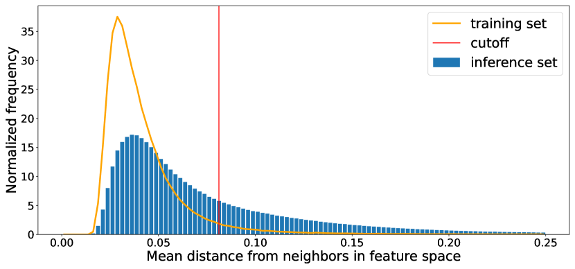
The red vertical line indicates the cut off distance value which corresponds to the 95th percentile. Next, using the previously determined K nearest neighbors model we calculated the distance of each inference data point from the 20 nearest neighbors lying in the training set, and again we calculated the mean of these distances. This way we can accurately determine the overlapping region of the training and inference sets in the feature space. We plotted the distribution of the distances denoted by blue bars in Figure 1. Altogether 2,879,298 from the total 4,849,611 quasar candidates in the inference set are closer to the training set than the cut off value. This means that the photometric redshift estimation based on our training set is the most reliable on this subset of the quasar candidates, otherwise we extrapolate into a less represented region.

We trained an XGBoost regressor (XGB) and an artificial neural network (ANN) on the complex relation between the feature space and the spectroscopic redshifts. We used XGB (Chen & Guestrin (2016)) as a baseline photo-z model and to measure the feature importances. XGB is a boosting algorithm that was developed on the basis of Gradient Boosting Decision Tree (Friedman (2001)). The main difference between the two models is that during the training phase XGB uses both of the first and second derivatives of the loss function. We set the number of estimators to 12 and the maximum depth to 15. The final photo-z catalogue was created however using the ANN, that outperformed XGB on the training set. We used four hidden layers each having 512 neurons and Exponential Linear Unit (ELU) activation function. ELU is more advanced than the widely used Rectified Linear Unit (RELU) since it solves the problem of vanishing gradient, while providing lower training times and higher accuracy. To avoid overfitting we added dropout layers after each hidden layer with a dropout rate of 0.2.

We created a photometric redshift catalog for a total number of 4,849,611 quasars including error estimation. From these, 2,879,298 quasars are within the training set coverage and therefore the redshift estimations are more reliable for them. We presented an XGBoost machine learning model as a base line method and used a more advanced artificial neural network model for the final predictions. We provided a detailed analysis of the results and an explanation for the observed bias in the data. Finally, we validated our redshift catalog using a completely independent, clustering-based redshift estimation method. We found good accordance between the results of the two methods below $z<2.5$ therefore the published catalog will be useful for several cosmological large-scale structure studies.

This work was supported by the Ministry of Innovation and Technology NRDI Office grants OTKA NN 129148 and the MILAB Artificial Intelligence National Laboratory Program. IS acknowledges support from the National Science Foundation (NSF) award 1616974.

The derived photometric redshift catalogue is publicly available at https://doi.org/10.5281/zenodo.6609756.

References

- Abate et al. (2012) Abate A., et al., 2012, Research report, Large Synoptic Survey Telescope: Dark Energy Science Collaboration, http://hal.in2p3.fr/in2p3-00748540. IN2P3, http://hal.in2p3.fr/in2p3-00748540
- Beck et al. (2016) Beck R., Dobos L., Budavári T., Szalay A. S., Csabai I., 2016, Monthly Notices of the Royal Astronomical Society, 460, 1371
- Benitez (2000) Benitez N., 2000, The Astrophysical Journal, 536, 571
- Blanton et al. (2017) Blanton M. R., et al., 2017, AJ, 154, 28
- Bolzonella et al. (2000) Bolzonella M., Miralles J. M., Pelló R., 2000, A&A, 363, 476
- Boris et al. (2007) Boris N. V., L. Sodre J., Cypriano E. S., Santos W. A., de Oliveira C. M., West M., 2007, The Astrophysical Journal, 666, 747
- Brammer et al. (2008) Brammer G. B., van Dokkum P. G., Coppi P., 2008, The Astrophysical Journal, 686, 1503
- Budavári (2009) Budavári T., 2009, The Astrophysical Journal, 695, 747
- Carliles et al. (2010) Carliles S., Budavári T., Heinis S., Priebe C., Szalay A. S., 2010, The Astrophysical Journal, 712, 511
- Chambers et al. (2016) Chambers K. C., et al., 2016, arXiv e-prints, p. arXiv:1612.05560
- Chen & Guestrin (2016) Chen T., Guestrin C., 2016, in Proceedings of the 22nd ACM SIGKDD International Conference on Knowledge Discovery and Data Mining. KDD ’16. Association for Computing Machinery, New York, NY, USA, p. 785–794, doi:10.1145/2939672.2939785, https://doi.org/10.1145/2939672.2939785
- Coe et al. (2006) Coe D., Benítez N., Sánchez S. F., Jee M., Bouwens R., Ford H., 2006, The Astronomical Journal, 132, 926
- Csabai et al. (2000) Csabai I., Connolly A. J., Szalay A. S., Budavári T., 2000, The Astronomical Journal, 119, 69
- Elliott et al. (2015) Elliott J., de Souza R., Krone-Martins A., Cameron E., Ishida E., Hilbe J., 2015, Astronomy and Computing, 10, 61
- Friedman (2001) Friedman J. H., 2001, The Annals of Statistics, 29, 1189
- Harikane et al. (2022) Harikane Y., et al., 2022, ApJ, 929, 1
- Hogan et al. (2015) Hogan R., Fairbairn M., Seeburn N., 2015, Monthly Notices of the Royal Astronomical Society, 449, 2040
- Ilbert, O. et al. (2006) Ilbert, O. et al., 2006, A&A, 457, 841
- Jin et al. (2019) Jin X., Zhang Y., Zhang J., Zhao Y., Wu X.-b., Fan D., 2019, Monthly Notices of the Royal Astronomical Society, 485, 4539
- Krone-Martins et al. (2014) Krone-Martins A., Ishida E. E. O., de Souza R. S., 2014, Monthly Notices of the Royal Astronomical Society: Letters, 443, L34
- Leistedt et al. (2016) Leistedt B., Mortlock D. J., Peiris H. V., 2016, Monthly Notices of the Royal Astronomical Society, 460, 4258
- Liu et al. (2006) Liu T., Moore A. W., Gray A., 2006, J. Mach. Learn. Res., 7, 1135–1158
- Lyke et al. (2020) Lyke B. W., et al., 2020, The Astrophysical Journal Supplement Series, 250, 8
- Magnier et al. (2020a) Magnier E. A., et al., 2020a, The Astrophysical Journal Supplement Series, 251, 3
- Magnier et al. (2020b) Magnier E. A., et al., 2020b, The Astrophysical Journal Supplement Series, 251, 5
- Magnier et al. (2020c) Magnier E. A., et al., 2020c, The Astrophysical Journal Supplement Series, 251, 6
- Ménard et al. (2013) Ménard B., Scranton R., Schmidt S., Morrison C., Jeong D., Budavari T., Rahman M., 2013, arXiv e-prints, p. arXiv:1303.4722
- Miles et al. (2007) Miles N., Freitas A., Serjeant S., 2007, in Ellis R., Allen T., Tuson A., eds, Applications and Innovations in Intelligent Systems XIV. Springer London, London, pp 75–87
- Nakoneczny, S. J. et al. (2021) Nakoneczny, S. J. et al., 2021, A&A, 649, A81
- O’Mill et al. (2011) O’Mill A. L., Duplancic F., García Lambas D., Sodré L., 2011, Monthly Notices of the Royal Astronomical Society, 413, 1395
- Schlafly et al. (2014) Schlafly E. F., et al., 2014, The Astrophysical Journal, 789, 15
- The Dark Energy Survey Collaboration (2005) The Dark Energy Survey Collaboration 2005, The Dark Energy Survey, doi:10.48550/ARXIV.ASTRO-PH/0510346, https://arxiv.org/abs/astro-ph/0510346
- Tonry et al. (2012) Tonry J. L., et al., 2012, ApJ, 750, 99
- Wadadekar (2005) Wadadekar Y., 2005, Publications of the Astronomical Society of the Pacific, 117, 79
- Waters et al. (2020) Waters C. Z., et al., 2020, The Astrophysical Journal Supplement Series, 251, 4
- Wright et al. (2010) Wright E. L., et al., 2010, The Astronomical Journal, 140, 1868
- Wu & Jia (2010) Wu X.-B., Jia Z., 2010, Monthly Notices of the Royal Astronomical Society, 406, 1583
- Yang et al. (2017) Yang Q., et al., 2017, The Astronomical Journal, 154, 269
- York et al. (2000) York D. G., et al., 2000, The Astronomical Journal, 120, 1579