Photometric Re-calibration of VPHAS+ -band Photometry with the Stellar Colour Regression Method and Gaia DR3
Abstract
The band magnitude is vital for determining stellar parameters and investigating specific astronomical objects. However, flux calibration in the band for stars in the Galactic disk presents significant challenges. In this study, we introduce a comprehensive re-calibration of -band photometric magnitudes of the VPHAS+ Data Release 4 (DR4), employing the Stellar Colour Regression (SCR) technique. By leveraging the expansive set of XP spectra and photometry from Gaia Data Release 3 (DR3), as well as the individual stellar extinction values provided by the literature, we have obtained precise model magnitudes of nearly 3 million stars. Our analysis identifies systematic magnitude offsets that exhibit a standard deviation of 0.063 mag across different observational visits, 0.022 mag between various CCDs, and 0.009 mag within pixel bins. We have implemented precise corrections for these observational visits, CCD chips, and pixel bins-dependent magnitude offsets. These corrections have led to a reduction in the standard deviation between the observed magnitudes and the model magnitudes from 0.088 mag to 0.065 mag, ensuring that the calibrated magnitudes are independent of stellar magnitude, colour, and extinction. The enhanced precision of these magnitudes substantially improves the quality of astrophysical research and offers substantial potential for furthering our understanding of stellar astrophysics.
keywords:
techniques: photometric – stars: fundamental parameters – catalogues1 Introduction
In recent years, numerous wide-field photometric surveys have been conducted (York et al., 2000; The Dark Energy Survey Collaboration, 2005; Skrutskie et al., 2006; Wright et al., 2010; Chambers et al., 2016; Gaia Collaboration et al., 2016; Zou et al., 2017; Onken et al., 2019; Željko Ivezić et al., 2019), producing revolutionary impacts on the advancement of astronomy. Uniform and high-precision flux calibration, which ensures a high degree of consistency in the flux measurements between targets that are widely separated in the sky and guarantees that these measurements do not vary with changes in the telescope’s working environment, detector position, or time of observation, is one of the key factors determining the success of wide-field surveys (Kent et al., 2009; Huang et al., 2022). The precision of flux calibration sets the lower limit on the error in stellar brightness measurements, which is significant for the determination of stellar photometric parameters, the selection of special astronomical objects, and the study of the structure of the Milky Way. Therefore, for the successful execution of wide-field photometric surveys, the undertaking of high-precision flux calibration is of utmost importance.
In traditional astronomical observations, absolute flux calibration is commonly performed using standard stars that are known to have a good internal consistency of brightness (Landolt, 1992; Yan et al., 2000; Zhou et al., 2001). However, due to a shortage of standard stars, the Forbes effect, the colour-dependent atmospheric extinction effect, and flat-field precision, the classical standard star method has difficulties to meet the milli-magnitude level calibration precision required by contemporary wide-field photometric surveys (Huang et al., 2022). In recent years, astronomers have developed a series of new flux calibration methods for wide-field photometric surveys. These methods typically focus only on the relative flux calibration process, with the absolute zero point still being provided by observing standard stars or calibrated to specific standard photometric systems. These include the Uber-calibration method (Padmanabhan et al., 2008), the Hyper-calibration method (Finkbeiner et al., 2016), the Forward Global Calibration Method (Burke et al., 2017), and the XP Synthetic Photometry method (Xiao et al., 2023b, 2024); as well as the Stellar Locus Regression method (High et al., 2009), Stellar Locus method (López-Sanjuan et al., 2019), and Stellar Colour Regression (SCR) method (Yuan et al., 2015; Huang & Yuan, 2022), among others.
Through the application of these methods, we have now achieved typical flux calibration precision of a few milli-magnitude in ground-based optical bands (Huang et al., 2022). However, the calibration precision in the near-ultraviolet band, especially for the band photometry in the Galactic disk, is still significantly larger than that in the optical bands. This is due to factors such as more significant atmospheric extinction effects in the band, more sensitive to stellar atmospheric parameters, lower detector response, fainter stellar magnitudes, insufficient numbers of standard stars, and more serious interstellar extinction effects in the Galactic disk. Nevertheless, the band is a very important part of stellar parameter determination and the identification of special astronomical objects. Previous work has attempted to accurately calibrate the band photometry for stars at high Galactic latitudes using stellar atmospheric parameters. Yuan et al. (2015) and Huang & Yuan (2022) have refined the band photometric calibration for the SDSS Stripe 82, achieving a precision of approximately 5 mmag in colour and magnitude, respectively. In a similar vein, Huang et al. (2021) managed to re-calibrate the band data for the SkyMapper Southern Survey at high Galactic latitudes with a precision of up to 1 per cent. Furthermore, the band photometry for the J-PLUS and S-PLUS surveys have been re-calibrated by Xiao et al. (2023c) and Xiao et al. (2023a), respectively, attaining calibration precision around of 5 mmag.
The VST Photometric H Survey (VPHAS+; Drew et al. 2014) uses VST/OmegaCAM to survey the Southern Galactic Plane and Bulge in , H down to magnitudes greater than 20. The band photometric data from VPHAS+ are essential for astronomical research, as they allow for the precise determination of stellar parameters near the Galactic centre and the study of the metallicity of the inner Galactic disk and the bulge. They are also crucial for the selection of OB stars in the inner Galactic disk. Chen et al. (2019b), using the VPHAS+ DR2 band data, identified nearly 27,000 candidates for O-type and early B-type stars, but due to the poor photometric precision, most of these sources were false positives. After validation with Gaia Data Release (DR2) data (Gaia Collaboration et al., 2018), of the nearly 27,000 candidates, only 6,858 were confirmed as candidates for O-type and early B-type stars.
The VPHAS+ observations concluded in 2018, and VPHAS+ Data Release (DR4) released catalogues of objects based on all observational data, including aperture magnitudes in the band for stars. The main goal of this paper is to assess the band photometric precision of stars in this VPHAS+ final data release and attempt to further calibrate the photometry. The structure of this paper is as follows: in Section 2, we introduce the data used; in Section 3, we present the methods employed. Our results are showcased and discussed in Section 4, and concluded in Section 5.


2 Data
2.1 VPHAS+
In this work, we present the utilization of the VPHAS+ DR4. This release encompasses observations conducted from 2015 to 2018. The data set includes reduced images and unstacked single-band source lists. The reduced images retain the original format of 32-CCD OmegaCam pawprints, covering a one-square-degree tile, and are not co-added. The single-band catalogues are derived from these images by the Cambridge Astronomical Survey Unit (CASU) pipeline.
For this study, we predominantly concentrate on -band photometry, archiving 1,544 catalogues including -band magnitudes. The number of objects detected in each catalogue varies significantly, with counts ranging from approximately ten thousand to hundreds of thousands, depending on the observed sky regions. Astrometric calibration was conducted with reference to the Two Micron All Sky Survey (2MASS) catalogue (Skrutskie et al., 2006), while photometric zeropoint calibration was performed nightly using standard stars. The astrometric precision within the data processing pipeline has a typical mean RMS error of 70 – 80 mas with respect to 2MASS. The source fluxes obtained were subjected to an illumination correction by cross-referencing with the AAVSO Photometric All-Sky Survey (APASS; Henden et al. 2009) stellar photometry, which, in turn, further refined the photometric zero-points. Reddening corrections were not applied to the data. The photometric calibration for the band is, however, relatively uncertain. The Vega band zeropoints are typically overestimated by about 0.3 mag, and the AB band zeropoints are extrapolated from longer wavelength bands, which can be unreliable under various atmospheric conditions111See the VPHAS+ DR4 release description via https://www.vphasplus.org/vphasplus-dr4-release-description.pdf.
2.2 Gaia
For further refinement of the VPHAS+ DR4 band photometric calibration, we incorporate data from Gaia Data Release 3 (DR3; Gaia Collaboration et al. 2023). We utilize the high-precision band photometric data and the low-resolution (BP/RP) XP spectra from Gaia DR3. The Gaia band spans wavelengths from 330 to 680 nm, providing photometry for approximately 1.5 billion stars. The calibration errors for the band are generally less than 1 mmag, as per the overall trend, except for very blue and bright sources (Riello et al., 2021; Yang et al., 2021). We have corrected the Gaia magnitudes following the methodology proposed by Yang et al. (2021).
Additionally, Gaia DR3 offers XP spectra for about 220 million stars (Carrasco et al., 2021; Gaia Collaboration et al., 2023). Rather than traditional pixelized wavelength-space measurements, the Gaia DR3 XP spectra are provided as sets of coefficients corresponding to 55 orthonormal Hermite functions for each of BP and RP spectra, resulting in a 110-dimensional coefficient vector for each stellar spectrum. For the purposes of our analysis, we require the spectral data in wavelength space to effectively exclude the influence of interstellar dust extinction. We have therefore transformed the Gaia DR3 XP spectra coefficients into wavelength space, utilizing the corrected spectra provided by Huang et al. (2024). These spectra have been resampled to a uniform wavelength grid spanning 392 to 992 nm, with a resolution of 10 nm, aligning with the methodology of Zhang et al. (2023b). We note that the band encompasses 320 – 390 nm, suggesting the utility of XP spectrum data below 390 nm. However, our decision to limit the spectrum range is driven by two primary considerations. First, the Gaia XP spectra display considerable noise near the boundaries of the BP and RP bands. The spectral data below 390 nm are characterized by elevated uncertainty levels, which could adversely affect the precision of our recalibration efforts. Second, we have incorporated the extinction values and extinction law from Zhang et al. (2023b), which are specifically defined for the wavelength range of 392 to 992 nm. This alignment enables direct comparison with their established extinction curve, which we utilize to ascertain the intrinsic stellar spectra. Despite omitting the spectra at lower wavelengths, the data from 392 - 992 nm are sufficient to accurately determine the intrinsic colours of the stars under study.
Given that the VPHAS+ survey areas are situated at low Galactic latitudes with high extinction values, the commonly used two-dimensional extinction maps (Planck Collaboration et al., 2014) tend to overestimate stellar extinction values in these regions. To address this, we adopt the stellar extinction values derived by Zhang et al. (2023b). They developed a forward model to estimate stellar atmospheric parameters (e.g., , , and ), distances, and extinctions for 220 million stars with XP spectra from Gaia DR3. They also provided an estimate of the optical extinction curve at the resolution of the XP spectra. Utilizing the extinction values and curve from Zhang et al. (2023b), we have obtained the intrinsic XP spectra for the individual stars.
2.3 Sample selection
We cross-match the VPHAS+ DR4 -band photometric catalogue with the Gaia DR3 within a matching radius of 1 arcsecond. To define our ‘Calibration Sample’ for flux calibration, we apply the following selection criteria:
-
1.
The source type from VPHAS+ is classified as a star with MERGEDCLASS = -1;
-
2.
The default VPHAS+ -band aperture-corrected magnitude is between 12 and 21.5 mag, and the magnitude errors are smaller than 0.08 mag;
-
3.
The Gaia phot_bp_rp_excess_factor is less than ;
-
4.
The Gaia XP spectra signal-to-noise ratio (SNR) for the full wavelength range is greater than 15;
-
5.
The extinction errors from Zhang et al. (2023b) are less than 0.02 mag.
Following these criteria, we have obtained a total of 2,974,582 stars for our Calibration Sample. From this sample, we further select a ‘Control Sample’ with relatively small dust extinction values. This sample is confined to a specific sky region defined by the following coordinates: right ascension RA deg, declination Dec deg, and Galactic latitude deg. The Control Sample comprises 18,002 stars. Fig. 1 illustrates the spatial distribution of stars in both the Calibration and Control Samples, as well as the total line-of-sight (LOS) extinction for these regions. Thanks to the extensive stellar count and all-sky distribution of stars provided by the Gaia XP spectra catalogue, we have obtained a substantial VPHAS+ -band Calibration Sample. This sample is distributed across each -band observation visit, a feat unachievable with traditional SCR methods which adopt spectroscopic catalogues. The extinction values are derived from two-dimensional extinction maps by Planck Collaboration et al. (2014). The areas covered by the VPHAS+ survey generally exhibit significant LOS extinction. We selected areas with relatively low LOS extinction as reference regions to minimize the impact of extinction on the -band photometric precision, thus obtaining a reference sample with more uniform photometry. The maximum extinction in the Control Sample region does not exceed 0.4 mag.
3 Method
In this work, we adopt an updated SCR (Yuan et al., 2015) method. Unlike the initial implementation of SCR, which predicted intrinsic stellar colours based on stellar atmospheric parameters such as effective temperature and metallicity [Fe/H] from spectroscopic surveys, our method predicts intrinsic stellar colours from intrinsic Gaia XP spectra. The detailed methodology employed is as follows.
-
1.
We begin by establishing the relationship between a star’s intrinsic XP spectrum and its intrinsic colour using the selected Control Sample. When obtaining the intrinsic XP spectra, we have applied a fixed extinction coefficient at each wavelength, sourced from Zhang et al. (2023b). This approach is justified given that the wavelength range corresponding to each flux measurement is only 10 nm. However, to obtain the intrinsic colour , considering the broad band and the band that covers the near-ultraviolet portion of the stellar SED where variations are prominent, the extinction coefficient cannot be assumed as a constant (e.g., Zhang & Yuan 2023; Sun et al. 2023). Here, is the extinction from Zhang et al. (2023b), and must at least vary with the effective temperature (or intrinsic colour) of the star. Initially, we use the extinction coefficient values provided by Zhang et al. (2023b) as a starting point for calculating the intrinsic colour .
After establishing the intrinsic colour , we employ a machine learning method, random forest regression (RFR), to train the relationship between the intrinsic XP spectra and . We randomly divide the Control Sample, using 75% for training and 25% for testing. The RFR model’s input parameters are the standardized intrinsic XP spectra (, where and are the original and standardized fluxes, respectively, and and are the mean and standard deviation). The output parameter is . This study uses the Python SCIKIT-LEARN package (Pedregosa et al., 2011) to train the RFR model. After testing a range of RFR model parameters, we select the best-performing set for training.
-
2.
The RFR model obtained from the previous step will be applied to the intrinsic XP spectra of stars in the Calibration Sample to obtain the predicted colour . Thus, we can determine the reddening value for each star in the Calibration Sample as . By combining this with the extinction values provided by Zhang et al. (2023b), we can fit the extinction coefficient and the zero-point offset . We use the following formula to relate to :
(1) where is the intrinsic colour , , , and are coefficients describing how the extinction coefficient varies with intrinsic colour , and represents the zero-point differences between the control and calibration samples. We iterate this step with the newly obtained extinction coefficients fed back into step (i), limiting the iterations to no more than five, as results generally stabilize after two or three iterations.
-
3.
With the relationship between intrinsic stellar spectra and colours obtained in step (i), and the extinction coefficient obtained in step (ii), we can predict the model magnitudes for each star in the Calibration Sample:
(2) The magnitude offsets between the model and observed magnitudes can then be determined using:
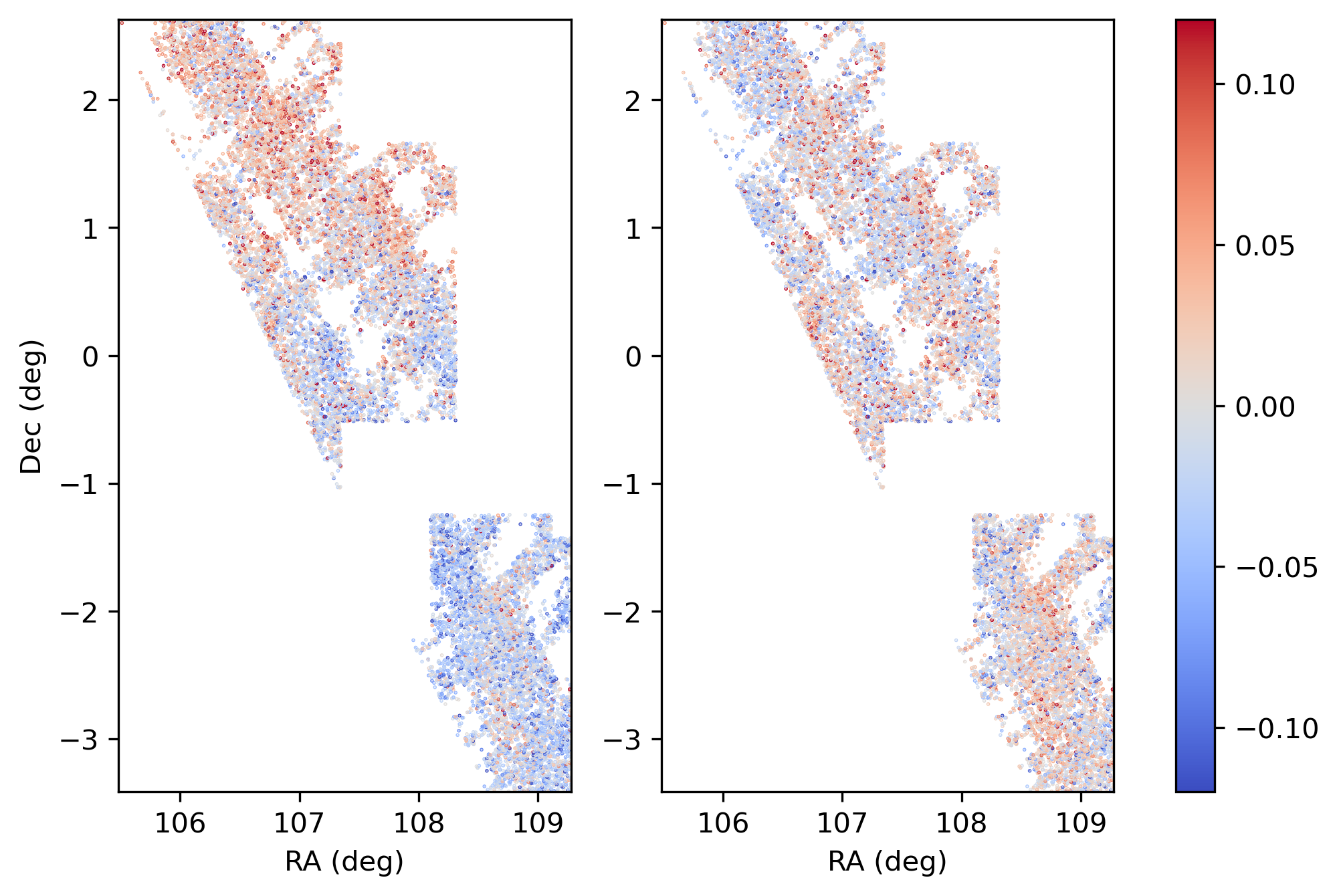
(3) After obtaining the initial magnitude offsets , we have performed a preliminary photometric calibration on the Control Sample to achieve a more uniform photometry across the reference stars. This preliminary calibration entails a straightforward adjustment of the zero-point differences in the magnitudes observed during each visit. We have computed the average for the Calibration Sample stars across each observational visit and applied the correction to derive the calibrated -band magnitudes: , where and are the post- and pre-calibration -band magnitudes respectively, and represents the average magnitude offset for each observational visit. The corrected magnitudes are then fed back into step (i) to iterate the calibration process.
Fig. 2 illustrates the spatial distribution of the for the Control Sample both before and after the preliminary flux calibration following the first iteration. Prior to the correction, a clear spatial variation in the magnitude offsets can be observed, with larger offsets in the upper-left region of the Diagram (Dec deg) compared to the lower-right region (Dec deg). The post-correction panel shows a more uniform distribution of magnitude offsets across different visits.


4 Result and discussion
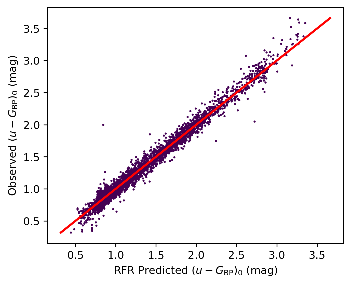
We first present some intermediate results obtained during the process of deriving the -band model magnitudes. For training, a subset consisting of 25 per cent of the Control Sample is randomly selected as the test sample to gauge the performance of our RFR model. Fig. 3 displays a comparison between the intrinsic colours predicted by our RFR model for the test sample stars and the observed values. The prediction closely matches the observations with a consistency parameter, the score, reaching 0.98. The dispersion between predicted and observed values is 0.064 mag. This outcome aligns with our expectations since the intrinsic XP spectra of stars contain essential information about their atmospheric parameters and intrinsic colours. In modelling the intrinsic colours, we utilized spectral fluxes directly, avoiding possible systematic errors inherent in measuring atmospheric parameters (Shen et al., 2022; Yang et al., 2024).
Fig. 4 shows the relationship between the reddening values for the Calibration Sample stars and the values from Zhang et al. (2023b). There are clear differences in the values for stars of different intrinsic colours (or effective temperatures). Our fitted results, based on Equation (1), correspond well with the data. The fitted relation for the extinction coefficient is as follows:
| (4) |
The magnitude difference between the Control Sample and the Calibration Sample is determined to be 0.009 mag.
4.1 Validating the -band photometric calibration
4.1.1 Magnitude differences across observational visits
Upon calculating the magnitude discrepancy, , for each star within our Calibration Sample, we proceed to investigate the consistency of this discrepancy across separate observational visits. Fig. 5 illustrates the spatial variability of the average values (denoted as ) relative to equatorial coordinates for each visit. A clear large-scale spatial variation in magnitude differences is evident, where (visit) values tend to be similar within adjacent sky regions at the same declination. However, there is a more significant variation across different right ascension intervals. For instance, (visit) is notably smaller in regions with RA 250 deg, and significantly larger within the 150 RA 175 deg interval.
We have also examined the temporal evolution of (visit), as depicted in the upper panel of Fig. 6. The mean magnitude difference exhibits a distinct seasonal trend. This trend is more pronounced in the bottom panel of Fig. 6, which shows the dispersion of magnitude differences over time for each observational visit. Typically, starting from October of each observing season, which corresponds to the Southern Hemisphere’s spring, the mean value of (visit) approaches zero with a smaller dispersion, approximately 0.1 mag. As time progresses, the mean increasingly deviates from zero, and the dispersion grows, reaching its maximum during the summer. These variations in (visit) with time and space reflect the unaccounted observational conditions, such as seeing and atmospheric quality, during photometric measurements. Quantitatively, the mean and standard deviation of are mag and mag, respectively.
4.1.2 Magnitude differences across individual CCD chips
We have then corrected the observed magnitude differences (visit) for each target field, obtaining a new set of corrected magnitudes (visit). These newly derived magnitudes should exhibit greater uniformity across both large spatial scales and over time, though discrepancies may persist among different CCDs. To test for systematic photometric calibration differences across the CCD array, we have compiled the CCD identifiers of each Calibration Sample star as well as their and image coordinates. We then examine the mean stellar magnitude difference averaged across different CCDs for each visit.
Fig. 7 displays the distribution of these mean magnitude discrepancy values, , for two arbitrarily selected observation sessions across different CCDs within the field of view (FOV). Post-correction for (visit) on a large spatiotemporal scale, the new (CCD, visit) values show reduced variation across different CCDs, generally lying within the range of to mag. However, these variations also exhibit temporal fluctuations.
Fig. 8 illustrates the time evolution of the mean magnitude differences (CCD, visit) for eight selected CCDs. CCDs numbered 1 through 4 reside at the FOV periphery (positioned in the lower-left quarter as depicted in Fig. 7), while CCDs 25 through 28 are situated nearer to the FOV center. These figures collectively unmask a gradual, long-term shift in the mean magnitude discrepancy, (CCD, visit). This could be attributed to variations in the gain factors of the individual CCDs, as well as to imperfections in the flat-field correction process. The computed mean and standard deviation of (CCD, visit) across the entire ensemble of CCDs for all observational visits are mag and mag, respectively.
4.1.3 Magnitude differences across individual pixel bins
The performance and accuracy of CCDs in astronomical observations can be influenced by a multitude of factors. These include, but are not limited to, electronic bias, defective pixels, pixel response non-uniformity, electronic interference, and variations in the optical throughput of the telescope system. Moreover, despite careful dark current subtraction and flat-field correction, some residual noise and non-uniform response may persist. This can introduce intermediate-scale flux variations in the astronomical data, potentially impacting the scientific interpretation of the measurements.
Corrections to the observed magnitude differences are also applied for each CCD chip to derive new corrected magnitudes . We compile observational data for each observing quarter, which corresponds to a one-year span, and scrutinize the new magnitude differences for stars in the Calibration Sample across individual pixels within each CCD. To reduce the influence of stochastic errors, we group stars within each pixel area and calculate the mean magnitude offset, .
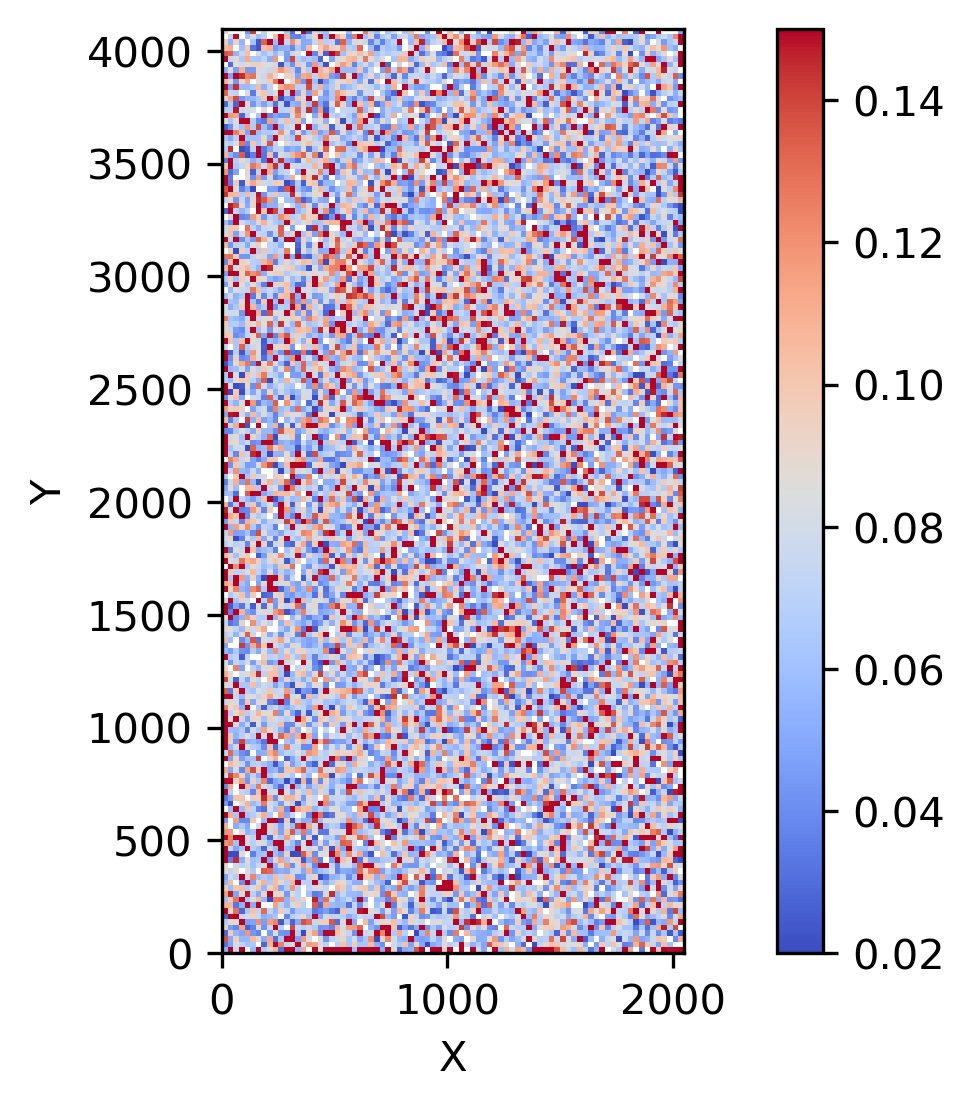
Fig. 9 illustrates the spatial distribution of values across the pixel coordinates for CCDs numbered 1 and 25, encompassing four years of observational quarters. Within an individual CCD, the average uncovers small-scale patterns—evident as larger values at the top of CCD 1 and smaller ones at the bottom, with an opposite pattern for CCD 25. Remarkably, these structural features persist with consistency through various observing quarters, suggesting intrinsic, temporally stable attributes.
In Fig. 10, we amalgamate the data from all observing quarters and visualize the variation of the mean magnitude difference, , within each CCD using the same pixel binning scheme. The resulting patterns of magnitude offset variation display pronounced values at the periphery of the FOV and at the centre of the entire field. The composite mean and standard deviation of across all pixels are mag and mag, respectively.
Finally, We turn our attention to the variability of individual star magnitude differences across the CCD array. Within a given CCD, a star’s magnitude difference can fluctuate by as much as mag. Moreover, nearly all CCDs exhibit faint structural features, characterized by two horizontal and two vertical bands, which are indicated by black arrows in Fig. 11.
For a detailed analysis, we compute the mean magnitude differences and their standard deviations within each pixel bin. The results suggest that these features become less pronounced, to the point of being nearly indiscernible, upon averaging. Stars aligned with these features tend to show marginally lower mean magnitude differences and slightly higher standard deviations.
In pursuit of the origins of these patterns, we have examined a selection of processed scientific images along with their respective twilight flat field images. However, these structural features are not apparent in the inspected images. Consequently, the origins of the faint horizontal and vertical bands remain elusive and are the subject of ongoing investigation.
Furthermore, we have identified a pronounced anomaly in the lower right corner of CCD 11, characterized by lower mean magnitude differences and increased standard deviations. It is depicted by a blue arrow in the mean value diagram and a red arrow in the standard deviation diagram in Fig. 11. This aberration corresponds to a defective column on the CCD chip, a flaw that is readily apparent in the downloaded images.
4.2 Enhancing the -band photometric calibration
In light of the findings presented earlier, we have refined the photometric calibration of the VPHAS+ -band data. We introduce a correction that is dependent on the individual visits, CCDs, and pixels to enhance photometric accuracy. The corrected -band magnitudes () are calculated as follows:
| (5) |
where represents the observed magnitude, and , , and are the magnitude offsets averaged by the visits, CCDs, and pixel bins, respectively. These offsets are derived in the previous section. We calculate these offsets only when a minimum of 20 stars from the Calibration Sample is present within the visit, CCD, or pixel bin. We have not applied corrections for a subset of stars (1.6 per cent of the Calibration Sample, amounting to 46,135 stars) due to the lack of sufficient star counts within their corresponding visit, CCD, or pixel bin.
The term is akin to a flux calibration zero point. In this work, we have chosen to utilize model magnitudes as reference standards to compute . This computation involves selecting stars that fall within the magnitude range of mag, the colour index range of mag, and have extinction values less than mag. We then average the magnitude offsets for this subset of stars to determine the zero point . Our findings yield a photometric zero point of mag.
Fig. 12 illustrates the post-correction magnitude offset, , as it relates to the stellar magnitude , colour index , and extinction . Consistent with our expectations, the post-correction magnitude offset generally approaches zero. Notable exceptions occur in regions with either a sparse stellar population or high extinction, which induce minor deviations from zero. We specifically select stars for which is nearest to zero, confined to the magnitude range mag, colour index range mag, and extinction mag. A Gaussian function is used to model the distribution of the magnitude offset both before () and after () the correction is applied. The fitting results, shown in Fig. 13, reveal that the pre-correction magnitude offset exhibits a systematic bias with a mean of mag and a standard deviation of 0.088 mag. The post-correction analysis demonstrates the elimination of the systematic bias and a reduction in the standard deviation to 0.065 mag. The improvement in photometric precision post-correction is approximately = 0.059 mag. This precision enhancement is consistent with the standard deviation of (visit), which is 0.063 mag (as shown in Fig. 6), which suggest that the systematic discrepancies in the VPHAS+ DR4 -band data have been successfully mitigated.
4.3 Estimation of Uncertainties in Model Magnitudes
In this section, we analyze the magnitude errors of our new SCR method. The sources of error in model magnitudes primarily stem from uncertainties in observational data, the fitting errors of intrinsic colours using the RFR model, and the quadratic function fitting errors associated with the extinction coefficients. To quantify the uncertainties associated with the model magnitudes, we have adopted a Monte Carlo (MC) simulation approach. The observational inputs include photometric uncertainties from the VPHAS+ band and Gaia band, flux measurement errors in Gaia XP spectra, and the uncertainties in extinction as reported by Zhang et al. (2023b). Our methodology involves defining two distinct sets of observational uncertainties: a ‘median set’ representing the median errors across all data, and a ‘90th set’ comprising errors at the 90th percentile, indicative of extreme error scenarios.
For the median set, the errors in , , and are 0.005 mag, 0.003 mag, and 0.014 mag, respectively, while the Gaia XP spectra have an SNR of 118. For the 90th set, the errors in , , and are 0.021 mag, 0.005 mag, and 0.019 mag, respectively, and the Gaia XP spectra have an SNR of 57. For each uncertainty set, we generate 10 MC realizations, resulting in a total of 20 MC samples.
By applying our SCR algorithm to these 20 MC data sets, we derive 20 corresponding sets of revised model magnitudes. The variability among these new magnitudes, when compared to our initial Calibration Sample-derived values, provides a statistical measure of the model magnitude uncertainties. The distributions of the magnitude differences for both the median and 90th set MC samples are presented in Fig. 14. Gaussian fits to these distributions indicate that the standard deviation is 0.027 mag for the median set and 0.036 mag for the 90th set.
It is important to note that in our MC analysis, we have not considered the potential impact of variations in the dust extinction law, specifically changes in the total-to-selective extinction coefficient (Zhang et al., 2023a). Additionally, we acknowledge that the -band magnitude errors reported in the VPHAS+ catalogue are significantly underestimated.
We have also calculated the -band model magnitudes for stars in the VPHAS+ catalogue by employing atmospheric parameters provided by the Apache Point Observatory Galactic Evolution Experiment (APOGEE; Majewski et al. 2017). These parameters include the effective temperature () and metallicity ([M/H]), following a methodology similar to that described by Xiao & Yuan (2022). Our analysis begins by selecting stars from the Sloan Digital Sky Survey Data Release 17 (SDSS DR17; Abdurro’uf et al. 2022) that have corresponding observations in APOGEE. These stars are then cross-matched with the VPHAS+ catalogue to form our primary dataset.
For the Calibration Sample, we have applied selection criteria that included: an SNR in APOGEE spectra greater than 20; in the range of 4300–5300 K; log values from 2.0 to 3.5 dex; and [M/H] greater than 1 dex. The Control Sample is further refined to include stars with right ascension less than 120 deg, declination greater than deg, and reddening values calculated from the APOGEE stellar parameters (Chen et al., 2019a; Sun et al., 2023) less than 0.5 mag. This selection process yields a total of 4,367 stars for the Calibration Sample and 532 stars for the Control Sample. We then determine the model magnitudes for the Calibration Sample using the same approach as Xiao & Yuan (2022).
Owing to the limited sample sizes of Calibration and Control Sample stars from APOGEE, we refrain from a direct comparison of these model magnitudes with those derived from Gaia XP spectra. Instead, we first compare the APOGEE-based model magnitudes with the observed VPHAS+ magnitudes to derive a magnitude offset. We proceed by computing the average magnitude offset for each VPHAS+ observation visit, denoted as . This is subsequently compared to the average offset obtained from the Gaia XP spectra. The comparative analysis, depicted in Fig. 15, demonstrates a strong agreement between the traditional SCR method utilizing APOGEE stellar parameters and the updated SCR method based on Gaia XP spectra. For observation visits with more than 20 stars, the standard deviation of the differences in between the two approaches is 0.036 mag.
5 Conclusions
Based on the corrected XP spectra (Huang et al., 2024) and the photometric data from Gaia DR3, along with the individual stellar extinction values provided by Zhang et al. (2023b), we have applied the novel SCR method to valid and enhance the photometric calibration of the -band magnitudes for the VPHAS+ DR4. In this work, we improve the previously established SCR approach by employing a machine learning technique, specifically RFR, to train the relationship between the extinction-corrected intrinsic XP spectra and the intrinsic stellar colours. Our method leverages the vast number of XP spectra available in Gaia DR3, effectively overcoming the limitations of traditional SCR methods, which rely heavily on spectroscopic survey data. As a result, we obtain a high-quality Calibration Sample of nearly 3 million stars, even for the surveys near the Galactic centre of VPHAS+. The RFR model, trained to predict the intrinsic colours of stars based on their XP spectra, shows remarkable consistency with the actual observations, achieving an score of 0.98. We also explore the relationship between colour excess and extinction values from Zhang et al. (2023b), observing how the extinction coefficients vary with intrinsic colour.
In this study, we have determined the model -band magnitudes for stars in our Calibration Sample. Through our analysis, we have unveiled spatial and temporal variations in the -band magnitude offsets within the VPHAS+ dataset, potentially linked to differing observational conditions. For each observational visit, the computed average magnitude offset, , exhibits a mean value of mag and a standard deviation of mag. Moreover, we have discerned variations in the magnitude offsets among different CCD chips within a single visit, which also fluctuate over time. These differences, denoted as , yield a mean value of mag and a standard deviation of mag. Additionally, we report the detection of consistent magnitude differences at the pixel level within each CCD, which appear to be stable over time, with a mean offset of mag and a standard deviation of mag.
Upon correcting for these varying magnitude offsets across observational visits (), CCD chips (), and pixel bins (), we have derived the revised -band magnitudes. These corrections led to a reduction in the standard deviation between the corrected magnitudes and the model magnitudes, decreasing from mag to mag. Notably, the corrected magnitudes exhibit no residual dependence on the stellar magnitude, colour, or extinction values. This improvement underscores the significance of our corrections and the enhanced reliability of the -band magnitude determinations as a result of this study.
Acknowledgements
This work is partially supported by the National Key R&D Program of China No. 2019YFA0405500, National Natural Science Foundation of China 12173034, 12322304, 12222301 and 12173007, and Yunnan University grant No. C619300A034. We acknowledge the science research grants from the China Manned Space Project with NO. CMS-CSST-2021-A09, CMS-CSST-2021-A08 and CMS-CSST-2021-B03.
This work is based on data products from observations made with ESO Telescopes at the La Silla Paranal Observatory under programme ID 177.D-3023, as part of the VST Photometric H Survey of the Southern Galactic Plane and Bulge (VPHAS+, www.vphas.eu).
This work has made use of data from the European Space Agency (ESA) mission Gaia (https://www.cosmos.esa.int/gaia), processed by the Gaia Data Processing and Analysis Consortium (DPAC, https://www.cosmos.esa.int/web/gaia/dpac/consortium). Funding for the DPAC has been provided by national institutions, in particular the institutions participating in the Gaia Multilateral Agreement.
Data availability
The data underlying this article is available in the manuscript.
References
- Abdurro’uf et al. (2022) Abdurro’uf et al., 2022, ApJS, 259, 35
- Burke et al. (2017) Burke D. L., et al., 2017, The Astronomical Journal, 155, 41
- Carrasco et al. (2021) Carrasco J. M., et al., 2021, A&A, 652, A86
- Chambers et al. (2016) Chambers K. C., et al., 2016, arXiv e-prints, p. arXiv:1612.05560
- Chen et al. (2019a) Chen B. Q., et al., 2019a, MNRAS, 483, 4277
- Chen et al. (2019b) Chen B. Q., et al., 2019b, MNRAS, 487, 1400
- Drew et al. (2014) Drew J. E., et al., 2014, MNRAS, 440, 2036
- Finkbeiner et al. (2016) Finkbeiner D. P., et al., 2016, The Astrophysical Journal, 822, 66
- Gaia Collaboration et al. (2016) Gaia Collaboration et al., 2016, A&A, 595, A1
- Gaia Collaboration et al. (2018) Gaia Collaboration et al., 2018, A&A, 616, A1
- Gaia Collaboration et al. (2023) Gaia Collaboration et al., 2023, A&A, 674, A1
- Henden et al. (2009) Henden A. A., Welch D. L., Terrell D., Levine S. E., 2009, in American Astronomical Society Meeting Abstracts #214. p. 407.02
- High et al. (2009) High F. W., Stubbs C. W., Rest A., Stalder B., Challis P., 2009, The Astronomical Journal, 138, 110
- Huang & Yuan (2022) Huang B., Yuan H., 2022, ApJS, 259, 26
- Huang et al. (2021) Huang Y., et al., 2021, ApJ, 907, 68
- Huang et al. (2022) Huang B., Xiao K., Yuan H., 2022, Scientia Sinica Physica, Mechanica & Astronomica, 52, 289503
- Huang et al. (2024) Huang B., et al., 2024, ApJS, 271, 13
- Kent et al. (2009) Kent S., et al., 2009, in astro2010: The Astronomy and Astrophysics Decadal Survey. p. 155 (arXiv:0903.2799), doi:10.48550/arXiv.0903.2799
- Landolt (1992) Landolt A. U., 1992, AJ, 104, 340
- López-Sanjuan et al. (2019) López-Sanjuan C., et al., 2019, A&A, 631, A119
- Majewski et al. (2017) Majewski S. R., et al., 2017, AJ, 154, 94
- Onken et al. (2019) Onken C. A., et al., 2019, Publ. Astron. Soc. Australia, 36, e033
- Padmanabhan et al. (2008) Padmanabhan N., et al., 2008, The Astrophysical Journal, 674, 1217
- Pedregosa et al. (2011) Pedregosa F., et al., 2011, Journal of Machine Learning Research, 12, 2825
- Planck Collaboration et al. (2014) Planck Collaboration et al., 2014, A&A, 571, A11
- Riello et al. (2021) Riello M., et al., 2021, A&A, 649, A3
- Shen et al. (2022) Shen H., Chen B. Q., Guo H. L., Yuan H. B., Sun W. X., Li J., 2022, MNRAS, 514, 4398
- Skrutskie et al. (2006) Skrutskie M. F., et al., 2006, The Astronomical Journal, 131, 1163
- Sun et al. (2023) Sun M., Chen B., Guo H., Zhao H., Yang M., Cui W., 2023, AJ, 166, 126
- The Dark Energy Survey Collaboration (2005) The Dark Energy Survey Collaboration 2005, arXiv e-prints, pp astro–ph/0510346
- Wright et al. (2010) Wright E. L., et al., 2010, The Astronomical Journal, 140, 1868
- Xiao & Yuan (2022) Xiao K., Yuan H., 2022, AJ, 163, 185
- Xiao et al. (2023a) Xiao K., et al., 2023a, arXiv e-prints, p. arXiv:2309.11533
- Xiao et al. (2023b) Xiao K., Yuan H., Huang B., Zhang R., Yang L., Xu S., 2023b, The Astrophysical Journal Supplement Series, 268, 53
- Xiao et al. (2023c) Xiao K., et al., 2023c, ApJS, 269, 58
- Xiao et al. (2024) Xiao K., et al., 2024, ApJS, 271, 41
- Yan et al. (2000) Yan H., et al., 2000, Publications of the Astronomical Society of the Pacific, 112, 691
- Yang et al. (2021) Yang L., Yuan H., Zhang R., Niu Z., Huang Y., Duan F., Fang Y., 2021, ApJ, 908, L24
- Yang et al. (2024) Yang L., Yuan H., Duan F., Zhang R., Huang B., Xiao K., Xu S., Zhang J., 2024, ApJS, 271, 37
- York et al. (2000) York D. G., et al., 2000, The Astronomical Journal, 120, 1579
- Yuan et al. (2015) Yuan H., Liu X., Xiang M., Huang Y., Zhang H., Chen B., 2015, The Astrophysical Journal, 799, 133
- Zhang & Yuan (2023) Zhang R., Yuan H., 2023, ApJS, 264, 14
- Zhang et al. (2023a) Zhang R., Yuan H., Chen B., 2023a, ApJS, 269, 6
- Zhang et al. (2023b) Zhang X., Green G. M., Rix H.-W., 2023b, MNRAS, 524, 1855
- Zhou et al. (2001) Zhou X., Jiang Z.-J., Xue S.-J., Wu H., Ma J., Chen J.-S., 2001, Chinese Journal of Astronomy and Astrophysics, 1, 372
- Zou et al. (2017) Zou H., et al., 2017, Publications of the Astronomical Society of the Pacific, 129, 064101
- Željko Ivezić et al. (2019) Željko Ivezić et al., 2019, The Astrophysical Journal, 873, 111