Photometric and Spectroscopic Observations of GRB 190106A: Emission from Reverse and Forward Shocks with Late-time Energy Injection
Abstract
Early optical observations of gamma-ray bursts can significantly contribute to the study of the central engine and physical processes therein. However, of the thousands observed so far, still only a few have data at optical wavelengths in the first minutes after the onset of the prompt emission. Here we report on GRB 190106A, whose afterglow was observed in optical bands just 36 s after the Swift/BAT trigger, i.e., during the prompt emission phase. The early optical afterglow exhibits a bimodal structure followed by a normal decay, with a faster decay after 1 day. We present optical photometric and spectroscopic observations of GRB 190106A. We derive the redshift via metal absorption lines from Xinglong 2.16-m/BFOSC spectroscopic observations. From the BFOSC spectrum, we measure . The double-peak optical light curve is a significant feature predicted by the reverse-forward external shock model. The shallow decay followed by a normal decay in both the X-ray and optical light curves is well explained with the standard forward-shock model with late-time energy injection. Therefore, GRB 190106A offers a case study for GRBs emission from both reverse and forward shocks.
1 Introduction
Since their discovery in the 1960s, the understanding of gamma-ray bursts (GRBs) has been greatly advanced by various space satellites and ground-based telescopes (see Zhang, 2018, for a review). Based on statistics of their prompt emission, GRBs are divided into two categories defined by their duration and spectral hardness, i.e., short bursts with hard spectra (also called type I bursts) with s and long bursts with soft spectra (also called type II bursts) with s (Kouveliotou et al., 1993; Zhang et al., 2009). The association of the short GRB 170817A with the gravitational wave event GW170817 confirmed the longstanding prediction (Eichler et al., 1989) that neutron star mergers can indeed produce short bursts (Abbott et al., 2017a, b; Zhang et al., 2018). Long GRBs are generally believed to originate from massive star collapse (Woosley & Bloom, 2006). GRB 980425/SN 1998bw demonstrated that some stellar collapses produce long bursts and broad-lined Type Ic supernovae (Galama et al., 1999). The comparison between long-duration GRBs and broad-lined SN rates suggests the ratio GRBs/CC-SNe is a few (Guetta & Della Valle, 2007).
Recent observations suggest that collapsing stars can also produce GRBs that last shorter than 2 s (Ahumada et al., 2021; Zhang et al., 2021; Rossi et al., 2022), compact star mergers seem to be also able to produce long GRBs (Rastinejad et al., 2022), indicating that classification of GRBs is more complex than the simple temporal division. Since its launch in 2004, the Neil Gehrels Swift Observatory (Swift hereafter) has detected more than 1700 GRBs with accurate position, enabling easy follow-up observations with ground-based telescopes (Gehrels et al., 2004). The typical isotropic equivalent energy (since it is the energy equivalent to the one that the GRB should have if the emission were isotropic) of GRBs ranges between ergs within a few seconds to minutes (Atteia et al., 2017). The jet break predicted by the collimated jet model has been observed in some GRBs, leading to the estimates of the true energy being orders of magnitude lower than the isotropic energy release (Frail et al., 2001).
Previous studies have shown that the X-ray light curves of GRB afterglows typically have several stages of power-law decay (): a steep decay phase (typically ), a shallow decay phase also called a plateau (typically ), a normal decay phase (typically ), a post-jet-break phase (typically ), with some bursts also accompanied by flares (Zhang et al., 2006). The typical optical light curve is an early rise followed by a normal decay, then sometimes followed by a re-brightening or a post-jet-break decay. Some long bursts, when at low enough redshift to allow a search, are found to be accompanied by a supernova bump (Zeh et al., 2004; Li et al., 2012).
In the standard model of GRBs, the afterglow is believed to involve a relativistically expanding fireball. Considering a relativistic thin shell with energy , initial Lorentz factor , opening angle , and a width in laboratory frame expanding into the interstellar medium (ISM) with density . The interaction between the shell and ISM is described by two shocks: 1) a forward shock (FS) propagating into the ISM. The shell first undergoes a coasting phase, where it moves at a nearly constant speed . It starts to decelerate and evolves into the second stage when the mass of the ISM swept by the forward shock is about of the rest mass of the shell. The third phase is the post-jet-break phase when the cone becomes larger than the geometric cone defined by . Finally, the blastwave enters the Newtonian phase (its velocity is much smaller than the speed of light) when it has swept up the ISM with the total rest mass energy comparable to the energy of the shell. During all these three phases, electrons are believed to be accelerated at the forward shock front to a power-law distribution . A fraction of the shock energy is distributed into electrons, and a fraction is in the magnetic field generated behind the shock. Accounting for the radiative cooling and the continuous injection of new accelerated electrons at the shock front, one expects a broken power-law energy spectrum of them, which leads to a multi-segment broken power-law radiation spectrum at any epoch (Gao et al., 2013, for a review). The typical afterglow observations are successfully described by the synchrotron emission of electrons from the forward shocks. However, the information of the properties of the fireball is lost in the forward shock, especially when it has been decelerated by the ISM; 2) a reverse shock (RS) propagating into the shell, which occurs in the very early afterglow epoch. In the thin shell case, the reverse shock is too weak to decelerate the shell effectively. The Lorentz factor of the shocked shell material is almost constant while the shock propagates in the shell. The reverse shock crosses the shell at the fireball deceleration time. At this time, the reverse and forward shocked regions have the same Lorentz factor and internal energy density. However, the typical temperature of RS is lower since the mass density of the shell is higher. Consequently, the typical frequency of RS is lower, and RS may play a noticeable role in the low-frequency bands, e.g., optical or radio (Mészáros & Rees, 1997). After the RS crosses the shell, the Lorentz factor of the shocked shell may be assumed to have a general power-law decay behavior . The shell expands adiabatically in the shell’s comoving frame. The emission from the RS is sensitive to the properties of the fireball. The observations of RS can thus provide important clues on the nature of the GRB source.
Catching very early (a few minutes after the trigger) optical emission from GRBs is not an easy task. There are only a few GRBs with optical observations during the prompt phase (Gao & Mészáros, 2015, for a review). Oganesyan et al. (2019) provided a sample of 21 GRBs with at least one observation during the prompt emission phase, and several GRBs in the sample are well observed (eg., GRB 070616, GRB 081008, GRB 121217A). Recently, Oganesyan et al. (2021) reported that they began to observe GRB 210619B 28s after the Swift trigger with D50 clear band during the prompt emission phase. However, our understanding of the earlier phases of GRBs continues to be quite incomplete compared to the later afterglow phases (occurring tens of minutes after the trigger).
In this paper, we report a special burst, GRB 190106A, for which optical observations began during the prompt emission phase, showing a double-peaked early optical light curve. We present optical photometric and spectroscopic observations of GRB 190106A with the NEXT (Ningbo Bureau Of Education And Xinjiang Observatory Telescope) and the Xinglong 2.16-m Telescopes. With the Xinglong 2.16-m/BFOSC spectroscopic observation, we present the redshift and calculate the equivalent widths of absorption lines in the afterglow spectrum. Combining our data with the Swift/XRT data and other observations from GRB Coordinates Network (GCN) reports, we constrain the parameters in an external shock model of the afterglow.
Our observations and data reduction are described in Section 2. The spectroscopic data analysis and redshift measurements are presented in Section 3. The optical and X-ray afterglow data analysis and the modeling of the afterglow light curve are reported in Section 4. We discuss possible models and present the conclusions in Section 5 and Section 6, respectively. A standard cosmology model is adopted with , =0.315, =0.685 (Planck Collaboration et al., 2014).
2 Observations
GRB 190106A triggered Neil Gehrels Swift Observatory (short as Swift) Burst Alert Telescope (BAT, Barthelmy et al. 2005) at 13:34:44 UT on 2019 Jan 06 (Sonbas et al., 2019). It is a long-duration burst with s. Konus-Wind also detected the burst with s (Tsvetkova et al., 2019). The MASTER-Amur robotic telescope quickly slewed to the burst position, starting observations 36 s after the BAT trigger. An optical transient (with a magnitude of 15.23 in the P-band) was discovered within the Swift/BAT error circle in the second 10 s exposure image (Yurkov et al., 2019; Lipunov et al., 2019) located at equatorial coordinates (J2000.0): , , consistent with the Swift/UVOT position , (Kuin & Sonbas, 2019). XRT and UVOT started observations at 81.8 s and 90 s after the BAT trigger, respectively. The BAT data files were downloaded from the Swift data archive111https://www.swift.ac.uk/swift_portal/. We extracted the BAT light curve and spectrum by the HEASoft software package (v6.27.2). The 15-150 keV spectra are analyzed in XSPEC (version 12.12) with power-law approximation over the time interval from 71 s to 81 s after the BAT trigger. We adopted the analysis results of the XRT repository products (Evans et al., 2007, 2009) and downloaded the 0.3-10 keV unabsorbed light curve from the UK Swift Science Data Centre222https://www.swift.ac.uk/xrt_curves/.
In our subsequent ground-based optical follow-up observations, the Xinglong 2.16-m obtained spectroscopic observations from which the redshift was determined (Xu et al., 2019), also confirmed by GMG (Mao et al., 2019) and X-shooter (Schady et al., 2019). We also collected observations from the GCNs reported by MASTER (Lipunov et al., 2019) and Sayan Observatory, Mondy (Belkin et al., 2019a, b). The MASTER data are converted to -band by adding mag following Xin et al. (2018). The corrected MASTER magnitude and Mondy optical observations are shown in Fig. 2 in gray color.


2.1 NEXT optical observations
NEXT is a fully automated telescope with a diameter of 60 centimeters, located at Nanshan, Xingming Observatory. NEXT is equipped with a E2V 230-42 back-illuminated CCD, and the CCD controller was made by the Finger Lakes Instrumentation (FLI). The size of the CCD is pixels, with a pixel size of . The pixel scale is , and the field of view (FOV) is according to the size of the CCD. The typical gain is , and typical readout noise is with readout speed. The equipped filters were in the standard Johnson-Cousins system.
NEXT is connected to GCN/TAN alert system, but did not observe GRB 190106A immediately as the dome was still closed at the very beginning of the event. NEXT began to obtain the first image at 13:57:21 UT, 22.6 minute after the BAT trigger, and the final one ended at 20:09:26 UT when the airmass was . The NEXT image of the burst location is also shown in Fig. 1. We obtained 88 images, all in the filter. Five of them were discarded for poor quality. The observing center time and exposure time of each image used are presented in Table 4.
The data reduction was carried out by standard processes in the IRAF packages (Tody, 1986), including bias, flat and dark current corrections. The cosmic rays were also removed by the filtering described in van Dokkum (2001). The final five useful images were combined using the task in IRAF. The astrometry was calibrated using Astrometry.net (Lang et al., 2010). The magnitudes were measured using (Bertin & Arnouts, 1996) using a circular aperture with a nine-pixel diameter. The photometric calibration was derived using the 14th data release (Abolfathi et al., 2018), with flux/mag conversion of the SDSS system into the Johnson-Cousins system333https://www.sdss.org/dr12/algorithms/sdssUBVRITransform/##Lupton. The light curve is shown in Fig. 2 and the photometric results are presented in Table 4.

2.2 Xinglong 2.16-m Observations
The spectroscopic observations were carried out with the National Astronomical Observatories, Chinese Academy of Sciences (NAOC) 2.16 m telescope (Fan et al., 2016) in Xinglong Observatory on 06 Jan 2019 at 14:02:39, minutes after the BAT trigger. The optical spectrum was obtained with the Beijing Faint Object Spectrograph and Camera (BFOSC) equipped with a back-illuminated E2V55-30 AIMO CCD. The optical afterglow magnitude was mag in R band and the airmass was approximately 1.3 at the beginning of the spectroscopic observations. Due to a seeing of about a slit-width of was used. The slit was oriented in a south-north direction. The grating used was G4 and the order-sorter filter 385LP was also used, leading to a spectral coverage of 3800 to 9000 Å at a resolution of about 10 Å. A total of two spectra were obtained with exposure time of 3600 s and 2400 s, respectively.
The BFOSC spectroscopic data were reduced by the IRAF standard processes to obtain clean images, including bias subtraction, flat-field correction and cosmic-ray removal. With the using of “NOAO” package provided in IRAF, we extracted the one-dimensional spectrum of the burst, and calibrated the wavelength with arc-spectra from an iron-argon lamp. The flux-calibration was performed by the standard star HD+19445 (Oke & Gunn, 1983) obtained with the same instrumental setup on the same night. After the processing above, the extracted spectrum is shown in Fig. 3.
The photometric observations were carried out on 7, 8 and 10 of Jan in the R filter again using the BFOSC (Fan et al., 2016). The exposure times were s, s, and s, respectively. The data reduction and processing was the same as NEXT, except dark current, which was negligible. The subsequent magnitude measurements were also performed as described above. The photometric data are presented in Table 4 and shown in Fig. 2. A comparison with a sample of historical GRB optical light curves is shown in Fig. 4.
3 Spectroscopic analysis
As the blue end of the BFOSC spectrum has poor signal-to-noise ratio, our spectral analysis starts at Å. After excluding the A and B band absorption and sky emission lines, we identified the metal absorption lines detected at more than significance. We detected lines from C IV, Al II, Al III, Fe II, and Mg II. Line centroids were determined by fitting a Gaussian function to the line profiles. We obtain a redshift of . The identified lines with the rest-frame equivalent widths () are listed in Table 5 and also shown in Fig. 3.

3.1 Line strength analysis
We analyzed the strong features of the GRB host galaxy interstellar medium detected by BFOSC, following de Ugarte Postigo et al. (2012). The Line Strength Parameter (LSP) of the spectrum is , which is very similar to the average value of the sample presented in the paper above. The line strength of the burst compared with the sample is shown in Fig. 5.

4 Optical and X-ray analysis and external shock Modeling
4.1 Temporal Analysis
The R-band, -ray and X-ray at 10 keV light curves are shown in Fig. 2. The optical light curve started at s and ended at d after the burst. According to the decay of the light curve, the optical and X-ray light curves can be divided into five and four stages, respectively. We fit the temporal indices of the light curves in Fig. 2 using .
The optical afterglow of the -band light curve can be divided into five stages with different decay indices, which are listed in Table 1, where the start and end times of different stages are also listed. The first stage is called fast rising, from the beginning of observation to s after the burst. This is followed by a fast decay until s. In the third stage (slow rising) it is still rising, the index has decreased by about 1 compared with the first stage. The fourth stage, normal decay, it starts from s and continues to s with a decay index of 0.63. In the final stage, late decay, the decay index increases to 1.29.
The light curve in X-rays seems simpler than in optical, and can be divided into the stages directly. The first stage is the tail of the prompt emission (steep decay) with a decay index of , observations started at s. It is followed by a shallow decay from s to s, with an index of 0.36. This stage can also be called a plateau phase, resulting from the small index. In the final stage, which called late decay, the decay index has increased to .
| Band | Segment | Start (s) | End (s) | |
| X-ray | steep decay | - | ||
| shallow decay | ||||
| late decay | - | |||
| Optical | fast rising | - | ||
| fast decay | ||||
| slow rising | ||||
| shallow decay | ||||
| late decay | - |
The BAT ( keV) count rates are also shown in the Fig. 2. The light curve can be simply divided into six episodes. The start, end and peak times of each episode are shown in Table 2. We note that between 71 s and 81 s of the prompt emission, the optical light curve has a similar evolutionary behavior: they all peak around 70 s and then fade. However, the peak time is slightly different, i.e., 76 s for , 76 s for X-ray, and 68 s for optical. The two high energy bands are almost simultaneous, but the optics peak about 8 s earlier. In addition, the BAT and XRT spectrum of this period can be described using a single power-law , and , , which is shown in Fig. 6. Although the UVOT optical data are not included in the spectral fitting, they are shown in the best-fit spectra in Fig. 6. As we see, the optical data are much lower than the extrapolation of the best spectral fits for high energies. The SED containing optical and high energy (X-ray, -ray) can’t be fitted by a single power-law.

| Episode | Start(s) | End(s) | Peak(s) | Duration(s) |
|---|---|---|---|---|
| Episode 1 | 0.2 | 9.2 | 2.8 | 9.0 |
| Episode 2 | 9.2 | 23.5 | 11.0 | 14.3 |
| Episode 3 | 50.6 | 57.1 | 52.1 | 6.5 |
| Episode 4 | 57.1 | 61.1 | 57.3 | 4.0 |
| Episode 5 | 71.0 | 75.2 | 73.3 | 4.2 |
| Episode 6 | 75.2 | 80.9 | 76.4 | 5.7 |
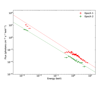
4.2 Afterglow SED analysis
To study the spectral energy properties of the afterglow, we select two epochs to construct its Spectral Energy Distribution (SED) with the best multi-band data: 28.8 ks (epoch 1) and 147.6 ks (epoch 2). The X-ray time sliced spectrum are obtained from the online repository444https://www.swift.ac.uk/xrt_spectra/, and the optical data are from Izzo et al. (2019) and Dichiara et al. (2019). We utilized the “grpph” tool of the Xspec package to re-bin the X-ray data to guarantee that each bin contains at least 20 counts to improve the SNR. We fit the spectrum by the power law function from “zdust*zphabs*phabs*powerlaw” model in the Xspec package, where “zdust” represents extinction by dust grains from the host galaxy of the burst, “zphabs” and “phabs” are neutral hydrogen photoelectric absorption of the host galaxy and Galaxy, respectively. The redshift and the Galactic hydrogen column is fixed to 1.86 and (HI4PI Collaboration et al., 2016), respectively. Small Magellanic Clouds extinction law is used as the host galaxy extinction model. The best fitted extinction E(B-V) of the host galaxy is 0.1 for epoch 1, which is also fixed in the fit of epoch 2. The best fitting result gives the photon index and for epoch 1 and 2, respectively. The results of these two epochs are shown in Fig. 7.
4.3 Theoretical Interpretation
The afterglow light curve of GRB 190106A is unusual. There is an optical flash followed by a second bump in the early optical light curve, and then a shallow decay followed by a normal decay. The X-ray light curve shows a steeper decay at the end of the prompt emission, followed by a shallow decay, and finally a normal decay.
To understand the multi-band observational data of GRB 190106A, we consider a relativistic thin shell with energy , initial Lorentz factor , opening angle , and a initial width in laboratory frame expanding into the ISM with density . The interaction between the shell and ISM is described by two shocks: an RS propagating into the shell and an FS propagating into the ISM (Rees & Meszaros, 1992; Mészáros & Rees, 1997; Sari et al., 1998; Sari & Piran, 1999; Zou et al., 2005). There are four regions separated by the two shocks: Region 1, the ISM with density ; Region 2, the shocked ISM; Region 3, the shocked shell material; Region 4, the unshocked shell material with density . First, the pair of shocks (FS and RS) propagating into the ISM and the shell, respectively. After the RS crosses the shell, the blastwave enters the deceleration phase. We now briefly describe these shocks separately.
The FS model we adopt was described in Lei et al. (2016). The dynamical evolution of the shell are calculated numerically using a set of hydrodynamical equations (Huang et al., 2000)
| (1) |
| (2) |
| (3) |
where and are the radius and time of the event in the burster frame, is the swept-up mass, is the ejecta mass, is the proton mass, and . The last equation might be replaced with (Geng et al., 2013)
| (4) |
when there is energy injection from GRB central engine. For , the injected power is , where is the initial injection power, is the decay power law index, and are the start and end time for energy injection. By solving these equations with the initial conditions, one can find the evolution of and .
During the dynamical evolution of FS, electrons are believed to be accelerated at the shock front to a power-law distribution . Assuming a fraction of the shock energy is distributed into electrons, this defines the minimum injected electron Lorentz factor,
| (5) |
where is electron mass. We also assume that a fraction of the shock energy is in the magnetic field generated behind the shock. This gives the comoving magnetic field
| (6) |
The synchrotron power and characteristic frequency from electron with Lorentz factor are
| (7) |
| (8) |
where is the Thomson cross-section, is electron charge. The peak spectra power occurs at
| (9) |
By equating the lifetime of electron to the time , one can define a critical electron Lorentz factor
| (10) |
the electron distribution shape should be modified for when cooling due to synchrotron radiation becomes significant. Accounting for the radiative cooling and the continuous injection of new accelerated electrons at the shock front, one expects a broken power-law energy spectrum of them, which leads to a multi-segment broken power-law radiation spectrum separated by three characteristic frequencies at any epoch (Gao et al., 2013, see Equations 15-17 therein).The first two characteristic frequencies and in the synchrotron spectrum are defined by the two electron Lorentz factors and . The third characteristic frequency is the self-absorption frequency , below which the synchrotron photons are self-absorbed (self-absorption optical depth larger than unity). The maximum flux density is , where is the total number of electrons in Region 2 (shocked ISM) and is the distance of the source.
Besides the numerical calculation of FS as described above, we can also provide an analytical description of the main properties of the evolution and emission of FS. Generally, the evolution includes four phases. The first is a coasting phase, in which we have . In the second phase, the shell starts to decelerate at the deceleration time
| (11) |
when the mass of the ISM swept by FS is about of the rest mass in the ejecta . After , the shell approaches the Blandford & McKee (1976) self-similar evolution and . Later, as the ejecta is decelerated to the post-jet-break phase at the time
| (12) |
when the cone becomes larger than . Finally, the blastwave enters the Newtonian phase when it has swept up the ISM with the total rest mass energy comparable to the energy of the ejecta. The dynamics is described by the well-known Sedov-Taylor solution. The synchrotron flux can be described by a series of power-law segments (Sari et al., 1998; Gao et al., 2013). For example, in the second phase (deceleration phase), and , one has the scalings for FS spectra parameters, i.e., , and (Gao et al., 2013, see Equation 49 therein). In the regime , one has . In the regime , one has (Gao et al., 2013, see Table 13 therein).
The RS model are described in Kobayashi (2000). In the thin shell case, the RS is Newtonian . The Lorentz factor of the shocked shell is nearly constant during the shock crossing the shell. The shell begins to spread around . The scalings before RS crossing time are (Kobayashi, 2000).
| (13) |
where is the total number of electrons in the ejecta.
We also assume that electrons are accelerated at the RS front to a power-law distribution , a fraction of the shock energy is distributed into electrons and a fraction to the magnetic field in Region 3. Follow the similar procedure as FS, we can obtain the scalings for parameters in the RS synchrotron spectrum (Gao et al., 2013, see Equation 26 therein),
| (14) |
In the regime , one has .
After the RS crosses the shell, i.e.,, the Lorentz factor of the shocked shell may be assumed to have a general power-law decay behavior . The shell expands adiabatically in the shell’s comoving frame. The dynamical behavior in Region 3 are expressed with the scalings (with ),
| (15) |
In the same way, we can obtain the scalings for parameters in the RS synchrotron spectrum for (Gao et al., 2013, see Equation 31 therein),
| (16) |
where is the cut-off frequency. After RS crossing, no new electrons are accelerated, will be replaced with . In the regime , one has .
In this section, we will show that the double-peak optical light curve as well the X-ray observations of GRB 190106A can be well-explained by synchrotron emission from reverse and forward shocks with late-time energy injection. We adopt a numerical code described above for both FS and RS to model the multi-band observational data. The modeled X-ray and optical light curves corresponding to the above-mentioned parameters (i.e., kinetic energy , initial Lorentz factor and opening angle of the relativistic shell, microphysics parameters for FS (,,) and RS (,,), and energy injection parameters (,,, ) ) are displayed in Fig. 8. However, these model parameters still suffer degeneracy when fitting the optical and X-ray data. In this work, we do not attempt to fit the data across a large parameter space. We present a set of parameter values that interpret the data well, as shown in Table 3. The subscripts “f ” and “r” denote the FS and RS emission, respectively.
4.3.1 Early Double-peak Optical Light curve
Zhang et al. (2003) pointed out that, depending on parameters, there are two types of early optical light curve for a fireball interacting with a constant-density ISM, that is, “rebrightening”, in which a distinct reverse-shock peak (with and , see the description of RS model above and also Tables 4 and 5 in Gao et al. (2013)) and forward-shock peak ( crossing peak) are detectable, and “flattening”, in which the FS peak is buried beneath the RS peak. The early optical light curve during the time span s post-trigger shows a double-peak feature, which is clearly a “rebrightening” case.
The first bump ( s) with rising temporal index and decay index can be interpreted as the combinations of a reverse-shock peak (see the blue dashed line in Fig. 8) and forward-shock emission (see the blue dotted line in Fig. 8). We find the results with can roughly explain such bump.
The first peak is also the RS crossing time (or deceleration time) . We can estimate the initial Lorentz factor , if we put and into Equation (11).
The second peak ( s) of the optical light curve occurs when the typical synchrotron frequency crosses the observed frequency (Sari et al., 1998). The slow-rising index of the second optical bump ( s) is consistent with emission below in a slow-cooling scenario, i.e., (Gao et al., 2013, see Table 13 therein). For such FS peak ( crossing peak), one has (Gao et al., 2013, see Equation 49 therein). The values of jet isotropic kinetic energy , ISM density and the microphysics parameter are chosen to fit this peak.
4.3.2 Shallow Decay Phase
GRB 190106A shows quite a long shallow decay in both X-rays (following the sharp decay) and the optical (following the second bump). In a slow-cooling regime of the forward shock, we expect for , which corresponds to using (Gao et al., 2013, see Table 13 therein) . Our observed values and are shallower than those expected. This phase can be understood within the standard external-shock model with nearly constant energy injection (see Fig. 8, and Xin et al. 2012 for a similar case). In Table 3, we present the parameter values that interpret the data well, i.e., the index , initial injection power , and starting time s. The energy injection shuts off at s.
There are two popular models for the energy injection, i.e., the spin-down of a magnetar and the fall-back accretion onto a stellar mass black hole (BH). First, we consider a fast-spinning magnetar as the central engine. The characteristic spin-down luminosity and the characteristic spin-down timescale are related to the magnetar initial parameters as (Zhang & Mészáros, 2001):
| (17) |
| (18) |
For the NS equation of state (EoS), we adopt EoS GM1 (the radius of the magnetar and the rotational inertia ) as suggested by the recent studies with GRB data (Lü et al., 2015; Gao et al., 2016). Inserting and into the above two equations, one can thus infer a magnetar initial period of ms and a magnetic field G.
For a black hole central engine model, the hyper-accreting BH system can launch a relativistic jet via neutrino-antineutrino annihilation (Popham et al., 1999; Narayan et al., 2001; Di Matteo et al., 2002; Janiuk et al., 2004; Gu et al., 2006; Chen & Beloborodov, 2007; Liu et al., 2007, 2015; Lei et al., 2009; Xie et al., 2016) or Blandford-Żnajek mechanism (hereafter BZ; Blandford & Żnajek 1977; Lee & Kim 2000; Li & Paczyński 2000; Lei et al. 2005, 2013). The neutrino annihilation mechanism is too “dirty” to account for a GRB jet (Lei et al., 2013; Xie et al., 2017). For this reason, we suppose that the energy injection is dominated by the BZ mechanism. The BZ power can be rewritten as a function of mass accretion rate as (Lei et al., 2013)
| (19) |
where is the dimensionless accretion rate, is the spin parameter of the BH, and . Assuming , the peak accretion rate is .
As we can see, both central engine models can give rise to the energy injection required. However, a fall-back accreting BH tends to produce a giant bump in GRB afterglow light curves (Wu et al., 2013). The plateau phase is a natural expectation from a magnetar central engine (Zhang & Mészáros, 2001; Lü et al., 2015). The small injection index (as shown in Table 3) favors the magnetar model.
4.3.3 Late Decay Phase
As shown in Table 1, just after the shallow decay phase, a break appears in X-ray at s and in optical light curve at s. Apparently, the X-ray break time is earlier than optical. In fact, this break time is affected by a large uncertainty. In Section 4.1, the X-ray light curve is divided into three segments, i.e., steep decay, shallow decay and late decay, as shown in Table 1. It can also be fit with four-segment broken power law: 1) steep decay (ends at s); 2) plateau (from s to s); 3) normal decay (from s to s); 4) late decay (starting from s) 555https://www.swift.ac.uk/xrt_live_cat/00882252/. In such case, the X-ray break time ( s) is roughly consistent with optical ( s). Therefore, the X-ray and optical breaking simultaneously cannot be ruled out.
The forward-shock model predicts temporal indices of and for optical and X-rays at late times, respectively, which correspond to and using (Gao et al., 2013, see Table 13 therein) . Our observed values and are larger than those expected.
Assuming that this break is due to the jet break, the predicted temporal index will become and by adopting . As shown in Fig. 8, our model can roughly fit the late time optical and X-ray light curves. Using this jet break time, we can estimate the opening angle if we inset erg, and s into the analytical expression Equation (12). As shown in Table 3, our numerical modeling gives the opening angle , which is slightly larger than this analytical estimation.

| Forward shock parameters | ||||||
| Reverse shock parameters | ||||||
| Energy injection parameters | ||||||
5 Discussion
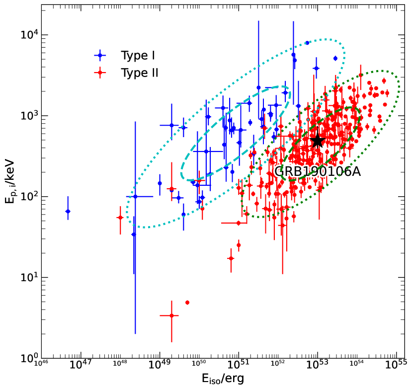

With the redshift measurement in this work, we tested the GRB by using two well-known relations, namely the Amati (Amati et al., 2002; Amati, 2006) and Yonetoku (Yonetoku et al., 2004) relations, as show in Fig. 9 left and right panel, respectively. The positions of the burst lie within the prediction regions, consistent with both Amati and Yonetoku relations, which is also mentioned by Tsvetkova et al. (2019). The result suggests that GRB 190106A is a typical type II GRB.
The early double-peak optical light curve was expected by Zhang et al. (2003). We show that GRB 190106A is a good case with reverse-forward shocks, just like GRB 041219A (Fan et al., 2005) and GRB 110205A (Zheng et al., 2012). Such double-peak (“rebrightening”) light curve is typical for RS+FS emission combinations in a homogeneous ISM case (Zhang et al., 2003; Kobayashi & Zhang, 2003). The rising temporal index favors the RS in thin-shell regime. Therefore, we adopted a thin-shell reverse-forward shock model in a constant ISM case to investigate GRB 190106A. In this scenario, the first optical peak (RS peak) gives the fireball deceleration time (Zhang et al., 2003), which can be used to estimate the initial Lorentz factor of the GRB, . The second optical peak appears when crosses the optical band. This peak flux can be used to constrain the values of jet isotropic kinetic energy , ISM density and the microphysics parameter . Based on the fit with this scenario, we infer that the magnetic field strength ratio in RS and FS is , suggesting a magnetic flux carried by the ejecta from the central engine. Therefore, a magnetized central engine model, i.e., a BH central engine powered by the BZ process or a magnetar central engine, is preferred in GRB 190106A.
It is worth to note that the first optical peak, like GRB 041219A, can be interpreted with a reverse shock (Fan et al., 2005), internal shocks (Vestrand et al., 2005; Wei, 2007), or tail emission (Panaitescu, 2020). The last two models assume that the prompt optical and -ray emissions have a common origin. However, the radiation mechanism for the prompt -ray emission is still poorly understood (Kumar & McMahon, 2008).
The shallow decays in both X-ray and optical bands demand a nearly constant late-time energy injection with and lasting from s to s. We investigated several energy injection sources, such as the spin-down of a magnetar, hyper-accreting BH powered by neutrino annihilation, and BH powered by BZ mechanism. The neutrino annihilation mechanism is less efficient for powering the jet at shallow decay phase. Both magnetar and BH central engine with BZ mechanism can give rise to the energy injection required. In general, the flat light curve feature favors the magnetar central engine model. A BH-accreting central engine can also makes a flat light curve, but requires a very small value of viscosity parameter (and thus a very slow accretion) (Lei et al., 2017). On the other hand, the disk will be dominated by advection and contains a strong wind at his afterglow phase. The light curve will then become steeper due to the suppression by the wind (Lei et al., 2017).
In Section 4.1, we divided the X-ray light curve into three stages (steep decay, shallow decay, late decay). As a result, the break time between shallow decay and late decay in X-ray is significantly different with that in optical band ( s vs s), as show in Table 1. However, the X-ray break time will be roughly consistent with optical if we fit the X-ray light curve with four segments (steep decay, plateau, normal decay, late decay). Considering this uncertainty, we attribute such break to the jet break, revealing an opening angle . From the observations and modeling, we found that the total jet energy is erg. The opening angle-corrected jet energy will be erg, which is well below the maximum rotational energy of erg (Lattimer & Prakash, 2016) erg (Haensel et al., 2009) for a standard neutron star with mass . Therefore, our data do not require a BH as the central engine of this GRB.
6 summary
We present our optical observation of the afterglow of GRB 190106A with the NEXT telescope, and the Xinglong 2.16-m telescope equipped with BFOSC. With the spectrum obtained from BFOSC, we measured the redshift of the burst and calculated the Line Strength Parameter. The unusual optical light curve obtained by NEXT and Xinglong 2.16-m, combined with the MASTER observations, show a normal decay light curve with early double peak and late break. Therefore, the optical light curve can be divided into five stages: rapid rise in the early stage, followed by decay, then a slow rise reaching a second peak at around 200 s, followed by a shallow decay (plateau), and faster decay from about 1 d onward. The evolution of the X-ray light curve can be divided more simply into three stages: rapid decay, plateau and normal decay.
The multi-band observations, especially the early optical data of GRB 190106A, provide rich information to study the nature of GRB. It is found that GRB 190101A can be successfully explained by the reverse-forward shock model. Our conclusions are summarized as follows:
1. The redshift of the burst is . The Line Strength Parameter, which is very similar to the average value of the sample.
2. The studies with the Amati and Yonetoku diagrams indicate that GRB 190106A is a typical type II burst.
3. The early double-peak optical light curve can be well interpreted with combination of the RS and FS models.
4. The modeling with RS and FS models indicate that the magnetic field strength ratio in RS and FS is , suggesting a magnetic flux carried by the ejecta from the central engine. This favors a strongly magnetized central engine model, such as a magnetar central engine model or a BH central engine powered by the BZ process.
5. The initial Lorentz factor can be estimated with the first optical peak time (or deceleration time) as .
6. The multi-band afterglow data can be interpreted with external shock model. From the observations and modeling, we found that the total jet energy is erg.
7. The shallow decays in both X-ray and optical bands are explained by nearly constant late-time energy injection with and lasting for s. Both magnetar and BH central engine models can give rise to such amount of injected energy, but the flat light curve feature favors a magnetar central engine.
8. The breaks at a few s in both X-ray and optical bands are roughly consistent with the jet break, revealing an opening angle . The opening angle-corrected jet energy will be erg.
acknowledgments
We are very grateful to Yong Ma for the help with the NEXT observations. We acknowledge the support of the staff of the Xinglong 2.16-m telescope. This work was also partially supported by the Open Project Program of the Key Laboratory of Optical Astronomy, National Astronomical Observatories, Chinese Academy of Sciences. This work is supported by the National Key R&D Program of China (Nos. 2020YFC2201400), the National Natural Science Foundation of China under grants U2038107, U1931203 and 12021003. D.X. acknowledges support by the science research grants from the China Manned Space Project with NO. CMS-CSST-2021-A13 and CMS-CSST-2021-B11. W. H. Lei and H. Gao acknowledge support by the science research grants from the China Manned Space Project with NO.CMS-CSST-2021-B11. W. Xie acknowledges support from the Guizhou Provincial Science and Technology Foundation (Grant No. QKHJC-ZK[2021] 027). H. Gao acknowledges support from the National SKA Program of China (grant No. 2022SKA0130101). J. Z. Liu acknowledges the science research grants from the China Manned Space Project with No. CMSCSST-2021-A08. Data resources are supported by the China National Astronomical Data Center (NADC) and the Chinese Virtual Observatory (China-VO). This work is supported by the Astronomical Big Data Joint Research Center, co-founded by the National Astronomical Observatories, the Chinese Academy of Sciences, and the Alibaba Cloud. We acknowledge the use of public data from the Swift data archive.
References
- Abbott et al. (2017a) Abbott, B. P., Abbott, R., Abbott, T. D., et al. 2017a, Phys. Rev. Lett., 119, 161101, doi: 10.1103/PhysRevLett.119.161101
- Abbott et al. (2017b) —. 2017b, ApJ, 848, L12, doi: 10.3847/2041-8213/aa91c9
- Abolfathi et al. (2018) Abolfathi, B., Aguado, D. S., Aguilar, G., et al. 2018, ApJS, 235, 42, doi: 10.3847/1538-4365/aa9e8a
- Ahumada et al. (2021) Ahumada, T., Singer, L. P., Anand, S., et al. 2021, Nature Astronomy, 5, 917, doi: 10.1038/s41550-021-01428-7
- Amati (2006) Amati, L. 2006, MNRAS, 372, 233, doi: 10.1111/j.1365-2966.2006.10840.x
- Amati et al. (2002) Amati, L., Frontera, F., Tavani, M., et al. 2002, A&A, 390, 81, doi: 10.1051/0004-6361:20020722
- Astropy Collaboration et al. (2022) Astropy Collaboration, Price-Whelan, A. M., Lim, P. L., et al. 2022, ApJ, 935, 167, doi: 10.3847/1538-4357/ac7c74
- Atteia et al. (2017) Atteia, J. L., Heussaff, V., Dezalay, J. P., et al. 2017, ApJ, 837, 119, doi: 10.3847/1538-4357/aa5ffa
- Barthelmy et al. (2005) Barthelmy, S. D., Barbier, L. M., Cummings, J. R., et al. 2005, Space Sci. Rev., 120, 143, doi: 10.1007/s11214-005-5096-3
- Belkin et al. (2019a) Belkin, S., Klunko, E., Pozanenko, A., et al. 2019a, GRB Coordinates Network, 23640, 1
- Belkin et al. (2019b) Belkin, S., Pozanenko, A., Minaev, P., et al. 2019b, GRB Coordinates Network, 23661, 1
- Bertin & Arnouts (1996) Bertin, E., & Arnouts, S. 1996, A&AS, 117, 393, doi: 10.1051/aas:1996164
- Blandford & McKee (1976) Blandford, R. D., & McKee, C. F. 1976, Physics of Fluids, 19, 1130, doi: 10.1063/1.861619
- Blandford & Żnajek (1977) Blandford, R. D., & Żnajek, R. L. 1977, MNRAS, 179, 433, doi: 10.1093/mnras/179.3.433
- Chen & Beloborodov (2007) Chen, W.-X., & Beloborodov, A. M. 2007, ApJ, 657, 383, doi: 10.1086/508923
- de Ugarte Postigo et al. (2012) de Ugarte Postigo, A., Fynbo, J. P. U., Thöne, C. C., et al. 2012, A&A, 548, A11, doi: 10.1051/0004-6361/201219894
- Dey et al. (2019) Dey, A., Schlegel, D. J., Lang, D., et al. 2019, AJ, 157, 168, doi: 10.3847/1538-3881/ab089d
- Di Matteo et al. (2002) Di Matteo, T., Perna, R., & Narayan, R. 2002, ApJ, 579, 706, doi: 10.1086/342832
- Dichiara et al. (2019) Dichiara, S., Gatkine, P., Durbak, J. M., et al. 2019, GRB Coordinates Network, 23744, 1
- Eichler et al. (1989) Eichler, D., Livio, M., Piran, T., & Schramm, D. N. 1989, Nature, 340, 126, doi: 10.1038/340126a0
- Evans et al. (2007) Evans, P. A., Beardmore, A. P., Page, K. L., et al. 2007, A&A, 469, 379, doi: 10.1051/0004-6361:20077530
- Evans et al. (2009) —. 2009, MNRAS, 397, 1177, doi: 10.1111/j.1365-2966.2009.14913.x
- Fan et al. (2005) Fan, Y. Z., Zhang, B., & Wei, D. M. 2005, ApJ, 628, L25, doi: 10.1086/432616
- Fan et al. (2016) Fan, Z., Wang, H., Jiang, X., et al. 2016, PASP, 128, 115005, doi: 10.1088/1538-3873/128/969/115005
- Frail et al. (2001) Frail, D. A., Kulkarni, S. R., Sari, R., et al. 2001, ApJ, 562, L55, doi: 10.1086/338119
- Galama et al. (1999) Galama, T. J., Vreeswijk, P. M., van Paradijs, J., et al. 1999, A&AS, 138, 465, doi: 10.1051/aas:1999311
- Gao et al. (2013) Gao, H., Lei, W.-H., Zou, Y.-C., Wu, X.-F., & Zhang, B. 2013, New A Rev., 57, 141, doi: 10.1016/j.newar.2013.10.001
- Gao & Mészáros (2015) Gao, H., & Mészáros, P. 2015, Advances in Astronomy, 2015, 192383, doi: 10.1155/2015/192383
- Gao et al. (2016) Gao, H., Zhang, B., & Lü, H.-J. 2016, Phys. Rev. D, 93, 044065, doi: 10.1103/PhysRevD.93.044065
- Gehrels et al. (2004) Gehrels, N., Chincarini, G., Giommi, P., et al. 2004, ApJ, 611, 1005, doi: 10.1086/422091
- Geng et al. (2013) Geng, J. J., Wu, X. F., Huang, Y. F., & Yu, Y. B. 2013, ApJ, 779, 28, doi: 10.1088/0004-637X/779/1/28
- Gu et al. (2006) Gu, W.-M., Liu, T., & Lu, J.-F. 2006, ApJ, 643, L87, doi: 10.1086/505140
- Guetta & Della Valle (2007) Guetta, D., & Della Valle, M. 2007, ApJ, 657, L73, doi: 10.1086/511417
- Haensel et al. (2009) Haensel, P., Zdunik, J. L., Bejger, M., & Lattimer, J. M. 2009, A&A, 502, 605, doi: 10.1051/0004-6361/200811605
- Harris et al. (2020) Harris, C. R., Millman, K. J., van der Walt, S. J., et al. 2020, Nature, 585, 357, doi: 10.1038/s41586-020-2649-2
- HI4PI Collaboration et al. (2016) HI4PI Collaboration, Ben Bekhti, N., Flöer, L., et al. 2016, A&A, 594, A116, doi: 10.1051/0004-6361/201629178
- Huang et al. (2000) Huang, Y. F., Gou, L. J., Dai, Z. G., & Lu, T. 2000, ApJ, 543, 90, doi: 10.1086/317076
- Hunter (2007) Hunter, J. D. 2007, Computing in Science & Engineering, 9, 90, doi: 10.1109/MCSE.2007.55
- Izzo et al. (2019) Izzo, L., Kann, D. A., de Ugarte Postigo, A., Blazek, M., & Thoene, C. C. 2019, GRB Coordinates Network, 23660, 1
- Janiuk et al. (2004) Janiuk, A., Perna, R., Di Matteo, T., & Czerny, B. 2004, MNRAS, 355, 950, doi: 10.1111/j.1365-2966.2004.08377.x
- Kann et al. (2010) Kann, D. A., Klose, S., Zhang, B., et al. 2010, ApJ, 720, 1513, doi: 10.1088/0004-637X/720/2/1513
- Kobayashi (2000) Kobayashi, S. 2000, ApJ, 545, 807, doi: 10.1086/317869
- Kobayashi & Zhang (2003) Kobayashi, S., & Zhang, B. 2003, ApJ, 597, 455, doi: 10.1086/378283
- Kouveliotou et al. (1993) Kouveliotou, C., Meegan, C. A., Fishman, G. J., et al. 1993, ApJ, 413, L101, doi: 10.1086/186969
- Kuin & Sonbas (2019) Kuin, N. P. M., & Sonbas, E. 2019, GRB Coordinates Network, 23626, 1
- Kumar & McMahon (2008) Kumar, P., & McMahon, E. 2008, MNRAS, 384, 33, doi: 10.1111/j.1365-2966.2007.12621.x
- Lang et al. (2010) Lang, D., Hogg, D. W., Mierle, K., Blanton, M., & Roweis, S. 2010, AJ, 139, 1782, doi: 10.1088/0004-6256/139/5/1782
- Lattimer & Prakash (2016) Lattimer, J. M., & Prakash, M. 2016, Phys. Rep., 621, 127, doi: 10.1016/j.physrep.2015.12.005
- Lee & Kim (2000) Lee, H. K., & Kim, H. K. 2000, Journal of Korean Physical Society, 36, 188. https://arxiv.org/abs/astro-ph/0008360
- Lei et al. (2005) Lei, W.-H., Wang, D.-X., & Ma, R.-Y. 2005, Chinese Journal of Astronomy and Astrophysics Supplement, 5, 279
- Lei et al. (2009) Lei, W. H., Wang, D. X., Zhang, L., et al. 2009, ApJ, 700, 1970, doi: 10.1088/0004-637X/700/2/1970
- Lei et al. (2016) Lei, W.-H., Yuan, Q., Zhang, B., & Wang, D. 2016, ApJ, 816, 20, doi: 10.3847/0004-637X/816/1/20
- Lei et al. (2013) Lei, W.-H., Zhang, B., & Liang, E.-W. 2013, ApJ, 765, 125, doi: 10.1088/0004-637X/765/2/125
- Lei et al. (2017) Lei, W.-H., Zhang, B., Wu, X.-F., & Liang, E.-W. 2017, ApJ, 849, 47, doi: 10.3847/1538-4357/aa9074
- Li et al. (2012) Li, L., Liang, E.-W., Tang, Q.-W., et al. 2012, ApJ, 758, 27, doi: 10.1088/0004-637X/758/1/27
- Li & Paczyński (2000) Li, L.-X., & Paczyński, B. 2000, ApJ, 534, L197, doi: 10.1086/312678
- Lipunov et al. (2019) Lipunov, V., Kuznetsov, A., Gorbovskoy, E., et al. 2019, GRB Coordinates Network, 23616, 1
- Liu et al. (2007) Liu, T., Gu, W.-M., Xue, L., & Lu, J.-F. 2007, ApJ, 661, 1025, doi: 10.1086/513689
- Liu et al. (2015) Liu, T., Hou, S.-J., Xue, L., & Gu, W.-M. 2015, ApJS, 218, 12, doi: 10.1088/0067-0049/218/1/12
- Lü et al. (2015) Lü, H.-J., Zhang, B., Lei, W.-H., Li, Y., & Lasky, P. D. 2015, ApJ, 805, 89, doi: 10.1088/0004-637X/805/2/89
- Mao et al. (2019) Mao, J., Xin, Y. X., Li, Y., et al. 2019, GRB Coordinates Network, 23630, 1
- Mészáros & Rees (1997) Mészáros, P., & Rees, M. J. 1997, ApJ, 476, 232, doi: 10.1086/303625
- Minaev & Pozanenko (2020) Minaev, P. Y., & Pozanenko, A. S. 2020, MNRAS, 492, 1919, doi: 10.1093/mnras/stz3611
- Narayan et al. (2001) Narayan, R., Piran, T., & Kumar, P. 2001, ApJ, 557, 949, doi: 10.1086/322267
- Nava et al. (2012) Nava, L., Salvaterra, R., Ghirlanda, G., et al. 2012, MNRAS, 421, 1256, doi: 10.1111/j.1365-2966.2011.20394.x
- Oganesyan et al. (2019) Oganesyan, G., Nava, L., Ghirlanda, G., Melandri, A., & Celotti, A. 2019, A&A, 628, A59, doi: 10.1051/0004-6361/201935766
- Oganesyan et al. (2021) Oganesyan, G., Karpov, S., Jelínek, M., et al. 2021, arXiv e-prints, arXiv:2109.00010. https://arxiv.org/abs/2109.00010
- Oke & Gunn (1983) Oke, J. B., & Gunn, J. E. 1983, ApJ, 266, 713, doi: 10.1086/160817
- Panaitescu (2020) Panaitescu, A. 2020, ApJ, 895, 39, doi: 10.3847/1538-4357/ab8bdf
- Planck Collaboration et al. (2014) Planck Collaboration, Ade, P. A. R., Aghanim, N., et al. 2014, A&A, 571, A16, doi: 10.1051/0004-6361/201321591
- Popham et al. (1999) Popham, R., Woosley, S. E., & Fryer, C. 1999, ApJ, 518, 356, doi: 10.1086/307259
- Rastinejad et al. (2022) Rastinejad, J. C., Gompertz, B. P., Levan, A. J., et al. 2022, arXiv e-prints, arXiv:2204.10864. https://arxiv.org/abs/2204.10864
- Rees & Meszaros (1992) Rees, M. J., & Meszaros, P. 1992, MNRAS, 258, 41, doi: 10.1093/mnras/258.1.41P
- Rossi et al. (2022) Rossi, A., Rothberg, B., Palazzi, E., et al. 2022, ApJ, 932, 1, doi: 10.3847/1538-4357/ac60a2
- Sari & Piran (1999) Sari, R., & Piran, T. 1999, ApJ, 520, 641, doi: 10.1086/307508
- Sari et al. (1998) Sari, R., Piran, T., & Narayan, R. 1998, ApJ, 497, L17, doi: 10.1086/311269
- Schady et al. (2019) Schady, P., Xu, D., Heintz, K. E., et al. 2019, GRB Coordinates Network, 23632, 1
- Schlafly & Finkbeiner (2011) Schlafly, E. F., & Finkbeiner, D. P. 2011, ApJ, 737, 103, doi: 10.1088/0004-637X/737/2/103
- Sonbas et al. (2019) Sonbas, E., Barthelmy, S. D., Beardmore, A. P., et al. 2019, GRB Coordinates Network, 23615, 1
- Tody (1986) Tody, D. 1986, in Society of Photo-Optical Instrumentation Engineers (SPIE) Conference Series, Vol. 627, Instrumentation in astronomy VI, ed. D. L. Crawford, 733, doi: 10.1117/12.968154
- Tsvetkova et al. (2019) Tsvetkova, A., Golenetskii, S., Aptekar, R., et al. 2019, GRB Coordinates Network, 23637, 1
- van Dokkum (2001) van Dokkum, P. G. 2001, PASP, 113, 1420, doi: 10.1086/323894
- Van Rossum & Drake (2009) Van Rossum, G., & Drake, F. L. 2009, Python 3 Reference Manual (Scotts Valley, CA: CreateSpace)
- Vestrand et al. (2005) Vestrand, W. T., Wozniak, P. R., Wren, J. A., et al. 2005, Nature, 435, 178, doi: 10.1038/nature03515
- Virtanen et al. (2020) Virtanen, P., Gommers, R., Oliphant, T. E., et al. 2020, Nature Methods, 17, 261, doi: 10.1038/s41592-019-0686-2
- Wei (2007) Wei, D. M. 2007, MNRAS, 374, 525, doi: 10.1111/j.1365-2966.2006.11156.x
- Woosley & Bloom (2006) Woosley, S. E., & Bloom, J. S. 2006, ARA&A, 44, 507, doi: 10.1146/annurev.astro.43.072103.150558
- Wu et al. (2013) Wu, X.-F., Hou, S.-J., & Lei, W.-H. 2013, ApJ, 767, L36, doi: 10.1088/2041-8205/767/2/L36
- Xie et al. (2016) Xie, W., Lei, W.-H., & Wang, D.-X. 2016, ApJ, 833, 129, doi: 10.3847/1538-4357/833/2/129
- Xie et al. (2017) —. 2017, ApJ, 838, 143, doi: 10.3847/1538-4357/aa6718
- Xin et al. (2012) Xin, L. P., Pozanenko, A., Kann, D. A., et al. 2012, MNRAS, 422, 2044, doi: 10.1111/j.1365-2966.2012.20681.x
- Xin et al. (2018) Xin, L.-P., Zhong, S.-Q., Liang, E.-W., et al. 2018, ApJ, 860, 8, doi: 10.3847/1538-4357/aabf3d
- Xu et al. (2019) Xu, D., Zhu, Z. P., Wang, Y., et al. 2019, GRB Coordinates Network, 23629, 1
- Yonetoku et al. (2004) Yonetoku, D., Murakami, T., Nakamura, T., et al. 2004, ApJ, 609, 935, doi: 10.1086/421285
- Yurkov et al. (2019) Yurkov, V., Gabovich, A., Sergienko, Y., et al. 2019, GRB Coordinates Network, 23614, 1
- Zeh et al. (2004) Zeh, A., Klose, S., & Hartmann, D. H. 2004, ApJ, 609, 952, doi: 10.1086/421100
- Zhang (2018) Zhang, B. 2018, The Physics of Gamma-Ray Bursts, doi: 10.1017/9781139226530
- Zhang et al. (2006) Zhang, B., Fan, Y. Z., Dyks, J., et al. 2006, ApJ, 642, 354, doi: 10.1086/500723
- Zhang et al. (2003) Zhang, B., Kobayashi, S., & Mészáros, P. 2003, ApJ, 595, 950, doi: 10.1086/377363
- Zhang & Mészáros (2001) Zhang, B., & Mészáros, P. 2001, ApJ, 552, L35, doi: 10.1086/320255
- Zhang et al. (2009) Zhang, B., Zhang, B.-B., Virgili, F. J., et al. 2009, ApJ, 703, 1696, doi: 10.1088/0004-637X/703/2/1696
- Zhang et al. (2021) Zhang, B. B., Liu, Z. K., Peng, Z. K., et al. 2021, Nature Astronomy, 5, 911, doi: 10.1038/s41550-021-01395-z
- Zhang et al. (2018) Zhang, Q., Lei, W. H., Zhang, B. B., et al. 2018, MNRAS, 475, 266, doi: 10.1093/mnras/stx3229
- Zheng et al. (2012) Zheng, W., Shen, R. F., Sakamoto, T., et al. 2012, ApJ, 751, 90, doi: 10.1088/0004-637X/751/2/90
- Zitouni et al. (2022) Zitouni, H., Guessoum, N., & Azzam, W. 2022, Ap&SS, 367, 74, doi: 10.1007/s10509-022-04100-2
- Zou et al. (2005) Zou, Y. C., Wu, X. F., & Dai, Z. G. 2005, MNRAS, 363, 93, doi: 10.1111/j.1365-2966.2005.09411.x
| (s) | Exp (s) | Filter | Mag (Vega) | Telescope | (s) | Exp (s) | Filter | Mag (Vega) | Telescope |
|---|---|---|---|---|---|---|---|---|---|
| 1387 | 60 | 16.92 +/- 0.02 | NEXT | 10661 | 200 | 18.27 +/- 0.04 | NEXT | ||
| 1482 | 60 | 16.98 +/- 0.02 | NEXT | 11109 | 200 | 18.39 +/- 0.05 | NEXT | ||
| 1569 | 60 | 17.01 +/- 0.02 | NEXT | 11337 | 200 | 18.41 +/- 0.05 | NEXT | ||
| 1673 | 90 | 17.05 +/- 0.02 | NEXT | 11564 | 200 | 18.36 +/- 0.05 | NEXT | ||
| 1786 | 90 | 17.10 +/- 0.02 | NEXT | 11791 | 200 | 18.40 +/- 0.05 | NEXT | ||
| 1898 | 90 | 17.11 +/- 0.02 | NEXT | 12017 | 200 | 18.39 +/- 0.05 | NEXT | ||
| 2068 | 200 | 17.24 +/- 0.01 | NEXT | 12239 | 200 | 18.42 +/- 0.05 | NEXT | ||
| 2291 | 200 | 17.30 +/- 0.02 | NEXT | 12462 | 200 | 18.42 +/- 0.05 | NEXT | ||
| 2513 | 200 | 17.42 +/- 0.02 | NEXT | 12733 | 300 | 18.47 +/- 0.04 | NEXT | ||
| 2786 | 300 | 17.45 +/- 0.02 | NEXT | 13052 | 300 | 18.45 +/- 0.04 | NEXT | ||
| 3105 | 300 | 17.53 +/- 0.02 | NEXT | 13370 | 300 | 18.41 +/- 0.05 | NEXT | ||
| 3425 | 300 | 17.64 +/- 0.02 | NEXT | 13688 | 300 | 18.43 +/- 0.05 | NEXT | ||
| 4063 | 300 | 17.76 +/- 0.02 | NEXT | 14005 | 300 | 18.50 +/- 0.05 | NEXT | ||
| 4388 | 300 | 17.80 +/- 0.02 | NEXT | 14321 | 300 | 18.52 +/- 0.05 | NEXT | ||
| 4654 | 120 | 17.77 +/- 0.03 | NEXT | 14637 | 300 | 18.47 +/- 0.04 | NEXT | ||
| 4799 | 120 | 17.84 +/- 0.03 | NEXT | 14955 | 300 | 18.55 +/- 0.05 | NEXT | ||
| 4945 | 120 | 17.86 +/- 0.03 | NEXT | 15272 | 300 | 18.62 +/- 0.05 | NEXT | ||
| 5089 | 120 | 17.90 +/- 0.03 | NEXT | 15589 | 300 | 18.61 +/- 0.06 | NEXT | ||
| 5236 | 120 | 17.94 +/- 0.04 | NEXT | 15905 | 300 | 18.69 +/- 0.06 | NEXT | ||
| 5381 | 120 | 17.90 +/- 0.03 | NEXT | 16222 | 300 | 18.63 +/- 0.05 | NEXT | ||
| 5529 | 120 | 17.92 +/- 0.03 | NEXT | 16539 | 300 | 18.54 +/- 0.05 | NEXT | ||
| 5675 | 120 | 17.98 +/- 0.04 | NEXT | 16855 | 300 | 18.48 +/- 0.05 | NEXT | ||
| 5912 | 200 | 18.00 +/- 0.03 | NEXT | 17172 | 300 | 18.62 +/- 0.06 | NEXT | ||
| 6138 | 200 | 17.97 +/- 0.03 | NEXT | 17489 | 300 | 18.52 +/- 0.05 | NEXT | ||
| 6363 | 200 | 18.04 +/- 0.03 | NEXT | 17806 | 300 | 18.59 +/- 0.06 | NEXT | ||
| 6589 | 200 | 18.01 +/- 0.03 | NEXT | 18123 | 300 | 18.61 +/- 0.07 | NEXT | ||
| 6813 | 200 | 18.09 +/- 0.03 | NEXT | 18440 | 300 | 18.41 +/- 0.06 | NEXT | ||
| 7042 | 200 | 18.05 +/- 0.03 | NEXT | 18756 | 300 | 18.68 +/- 0.07 | NEXT | ||
| 7267 | 200 | 18.10 +/- 0.03 | NEXT | 19074 | 300 | 18.64 +/- 0.07 | NEXT | ||
| 7491 | 200 | 18.14 +/- 0.03 | NEXT | 19391 | 300 | 18.63 +/- 0.07 | NEXT | ||
| 7717 | 200 | 18.12 +/- 0.03 | NEXT | 19709 | 300 | 18.84 +/- 0.09 | NEXT | ||
| 7946 | 200 | 18.16 +/- 0.03 | NEXT | 20025 | 300 | 18.83 +/- 0.10 | NEXT | ||
| 8172 | 200 | 18.12 +/- 0.03 | NEXT | 20342 | 300 | 18.85 +/- 0.10 | NEXT | ||
| 8397 | 200 | 18.12 +/- 0.03 | NEXT | 20658 | 300 | 18.75 +/- 0.10 | NEXT | ||
| 8624 | 200 | 18.23 +/- 0.04 | NEXT | 20975 | 300 | 18.72 +/- 0.10 | NEXT | ||
| 8852 | 200 | 18.28 +/- 0.04 | NEXT | 21292 | 300 | 18.96 +/- 0.13 | NEXT | ||
| 9078 | 200 | 18.30 +/- 0.04 | NEXT | 21609 | 300 | 18.84 +/- 0.12 | NEXT | ||
| 9302 | 200 | 18.28 +/- 0.04 | NEXT | 21925 | 19.12 +/- 0.12 | NEXT | |||
| 9529 | 200 | 18.32 +/- 0.04 | NEXT | 84911 | 19.77 +/- 0.06 | Xinglong 2.16-m | |||
| 9756 | 200 | 18.30 +/- 0.04 | NEXT | 165878 | 20.70 +/- 0.05 | Xinglong 2.16-m | |||
| 9980 | 200 | 18.31 +/- 0.04 | NEXT | 345290 | 21.73 +/- 0.06 | Xinglong 2.16-m |
| (Å) | Feature(Å) | (Å) | |
|---|---|---|---|
| 4428.26 | C IV/ C IV1549 | 1.859 | |
| 4604.72 | Fe II1608 | 1.864 | |
| 4776.51 | Al II1670 | 1.860 | |
| 5304.92 | Al III1854 | 1.861 | |
| 5329.60 | Al III1862 | 1.862 | |
| 6704.71 | Fe II2344 | 1.860 | |
| 6789.60 | Fe II2374 | 1.860 | |
| 6811.21 | Fe II2382 | 1.859 | |
| 7397.92 | Fe II2586 | 1.861 | |
| 7435.47 | Fe II2600 | 1.860 | |
| 8011.58 | Mg II/Mg II 2800 | 1.861 | |
| 8158.45 | Mg I 2852 | 1.861 |