[SM-]SM[SM.pdf]
Phonon-Mediated Nonlinear Optical Responses and Quantum Geometry
Abstract
Unraveling the complexities of nonlinear optical (NLO) responses, particularly the intricate many-body interactions among photons, electrons, and phonons, remains a significant challenge in condensed matter physics. Here, we present a diagrammatic approach to explore NLO responses with electron-phonon coupling (EPC), focusing on the phonon-mediated nonlinear optical (Ph-NLO) responses up to the second order in photon perturbation. We systematically analyze the shift and ballistic mechanisms responsible for phonon-mediated electron-photon interactions. By incorporating EPC effects, we elucidate phenomena such as phonon-mediated shift current (Ph-SC) and second-harmonic generation (Ph-SHG) in a comprehensive Ph-NLO framework. This approach enables below-gap resonant responses at terahertz photon frequencies, offering a promising mechanism for terahertz optical applications that surpasses the constraints of conventional pure-electronic NLO theories. Additionally, we explore the geometric and topological consequences of Ph-NLO responses by introducing the EPC Berry curvature, EPC quantum metric, and EPC shift vector. These concepts unveil a unique quantum geometric structure within the Hilbert space, parameterized by both the electronic wavevector and phonon-displacement, thereby extending the established pure-electronic quantum geometry. Using a general Rice-Mele model, we demonstrate the connection between Ph-NLO responses and EPC geometry, discussing the implications and predicting observable effects for future experimental validation. This framework also provides a foundation for advancing first-principles calculations aimed at the discovery and engineering of NLO materials. The insights gained from this study contribute to a more profound understanding of NLO responses and EPC quantum geometry.
- Keywords
-
nonlinear optical responses; electron-phonon coupling; Feynman diagram; quantum geometry
I Introductions
Nonlinear optics investigates the interactions between light and matter under high-intensity light conditions. Since its first observation in the late 19th century, nonlinear optics has seen substantial advancements [1, 2], offering promising applications in fields such as ultrafast optics [3], bulk photovoltaics (BPVE) [4, 5, 6], nonlinear optical (NLO) sensing and imaging [7], optical transistors [1], and efficient generation of entangled photon pairs for quantum computing [8].
One key area for advancement in nonlinear optics involves addressing the limitations of the resonant NLO frequency spectrum at low-energy ranges, where the incident photon’s energy must exceed the material’s band gap to excite electrons. Electron-phonon coupling (EPC) has emerged as a promising solution to this challenge. Previous studies have demonstrated the phonon-assisted inter-band optical absorption in silicon and BaSnO3 from both first-principles calculation and experiments as a first-order linear effect [2, 9], and phonon-assisted ballistic current as a second-order NLO effect [10]. More recently, strong second-order shift current signals have been observed in BaTiO3 with a resonant frequency far below the electronic band gap, suggesting a phonon-mediated mechanism [11]. Gu et al. also experimentally demonstrated phonon-assisted BPVE in MoSe2 [12], achieving enhanced performance. These findings indicate that the phonon-mediated linear and nonlinear optical (Ph-LO and Ph-NLO) responses are sensitive to the low-energy photons (in the meV range), which could greatly broaden the frequency response spectrum and hold substantial potential for THz applications.
Recent studies have deeply rooted nonlinear optics in the quantum geometry, which explores the geometric structure of the Hilbert space spanned by electronic eigenstates. A fundamental concept of quantum geometry is the quantum geometric tensor (QGT), also known as the Fubini–Study metric [13, 14]. This gauge-invariant tensor quantifies the geodesic distance between quantum states, encompassing both the symmetric quantum metric and the antisymmetric Berry curvature [15]. These quantities, along with extensions like the Berry curvature dipole and quantum metric dipole, serve as the foundation for various transport phenomena [16, 17, 18, 19, 20, 21, 22, 23, 24]. In nonlinear optics, the QGT plays a pivotal role in establishing direct connections with the inter-band optical transitions and optical absorption strength [25] and is extensively discussed in the NLO responses, including the photovoltaic effect [26, 27] and second-harmonic generation (SHG) [28], with particular emphasis on cases involving time-reversal-symmetry breaking [14] and low-frequency divergence [26]. On the experimental measurement of QGT, a Bloch-state tomography method has been developed to extract the QGT from an optical Raman lattice in ultracold atoms [29]. Furthermore, a direct measurement of the QGT has been conducted in an optically active system [30], underscoring the nontrivial band geometry [31].
In addition to the QGT, significant attention has been directed toward the Hermitian connection geometry [13] associated with even-order NLO responses, which is present exclusively in noncentrosymmetric materials [32, 33, 34, 35]. A key concept is the shift mechanism for the BPVE, which arises from the real-space displacement of charge carrier wave packets upon photon absorption. This effect is characterized by the shift vector [36, 37, 38], and is revealed in high-harmonic generation from noncentrosymmetric topological insulators [39]. Unlike extrinsic mechanisms, such as ballistic currents in the relaxation of excited carriers or p-n junctions, the intrinsic shift mechanism enables more efficient, near-instantaneous energy transfer with minimal dissipation [11, 40], making it promising for applications in solar cells and photodetectors [34, 41, 42, 40, 43].
Previous studies have predominantly concentrated on the geometric effect associated with the pure-electronic transition dipole moment. However, quantum geometry and nonlinear optics are deeply intertwined with many-body interactions, including those involving phonons and excitons. For instance, the nontrivial quantum geometry can enhance the strength of EPC in multi-band electron systems, highlighting the significance of electron band geometry and the Fubini-Study quantum metric in superconductivity [44]. The quantum metric is also crucial in governing the characteristics of single exciton excitations and exciton condensates [45]. Additionally, the shift current BPVE is influenced by quasiparticle and exciton [46]. Phonon can significantly influence the electronic states in various materials, particularly in ferroelectric (FE) systems. Recent studies have demonstrated that in systems with strong EPC, the amplitude of the ‘shift heat current’, as a type of heat current analog of the optical shift current, can be enhanced to the electronic energy scale, even when only phonons are excited by an external field [47].
Motivated by these insights, we present a comprehensive diagrammatic study of generalized Ph-NLO and EPC quantum geometry. We start with discussing the elementary vertices in Sec. II, followed by the derivation of two fundamental types of phonon-mediation vertices, namely the shift and ballistic types in Secs. III, based on which we propose the full Ph-NLO responses in Sec. IV up to the second order of photon perturbation. The phonon-mediated shift current (Ph-SC) and phonon-mediated second harmonic generation (Ph-SHG) are discussed as two special limits. We further reveal the EPC quantum geometry and its relation with Ph-NLO responses in Sec. V, along with further discussions on symmetry, the Rice-Mele model, and experimental measurement in Sec. VII. Our work aims to shed light on the development of Ph-NLO responses and its connection to quantum geometry.
| Symbol | Expression | Unit | Description |
|---|---|---|---|
| – | 1/s | Photon frequency polarized along -direction | |
| eV | Energy of (quasi) electronic state | ||
| - | eV | Energy of (quasi) phonon mode . | |
| eV | Electronic energy difference | ||
| 1 | Occupance of state at temperature | ||
| 1 | Occupance difference | ||
| eV | Zeroth-order EPC matrix element (:phonon mode) | ||
| eVÅ | First-order covariant derivative of Hamiltonian over | ||
| Å | Off-diagonal matrix element of positional operator | ||
| Å | Diagonal matrix element of positional operator | ||
| eVÅ2 | Second-order covariant derivative of Hamiltonian | ||
| eVÅ | First-order EPC matrix element | ||
| 1/eV | Electronic Green’s function projected on eigen-state | ||
| 1/eV | Phononic Green’s function projected on mode |
II Elementary vertices
We adopt the framework presented Ref [48] to describe the electronic states in a -dimensional crystalline material. The unperturbed electronic Hamiltonian is expressed as:
| (1) |
where refers to the normalized integral over the -dimensional first Brillouin zone (BZ) with unit cell volume , and is the band index. and ’s are single-particle fermion creation and annihilation operators. The single-electron wave functions is written as:
| (2) |
where are the periodic parts over unit cell, and serve as eigenfunctions of the Hamiltonian in -space :
| (3) |
The unperturbed phononic Hamiltonian is given by:
| (4) |
where is the phonon mode index. and ’s are single-particle bosonic creation and annihilation operators. For notation simplification, we incorporate the electronic wave vector and phononic wave vector into electron band index (typically labeled by Latin indices ) and phonon mode index , respectively, in subsequent discussions.
Next, we consider the electronic Hamiltonian with EPC:
| (5) |
where is the EPC operator for the -mode phonon, with representing the phonon displacement quantum, and denotes the partial derivative with respect to the phonon displacement (see further discussions in Appendix. A). The influence of to is renormalized into electronic self-energy , modifying the bare electron Green’s function -state as:
| (6) |
Similarly, EPC contributes to the phononic self-energy , which affects the -mode phonon Green’s function . In following discussions, and will not be explicitly written, as we assume the effects are included in the quasi-energies and , unless otherwise specified. The imaginary part of self-energy, which characterizes the lifetime of quasi-particles, will be discussed in the context of resonance analysis.
The light illumination is classically considered as the time-dependent electric field intensity . In the velocity gauge, the electric component of the electromagnetic field is defined from the vector potential as . The impact of is accounted for the electron-phonon system through the minimum substitution [48]:
| (7) |
Expanding in a Taylor series yields:
| (8) | ||||
In the frequency domain, with -direction electric field intensity , the Hamiltonian becomes:
| (9) | ||||
where are the covariant derivatives, and the Berry connections are denoted by with the partial derivative to -direction wave vector . The covariant derivative acts on any operator as [48]
| (10) |
with the matrix element:
| (11) |
We specifically denote the -order covariant derivative of unperturbed electronic Hamiltonian as: , and similarly for the EPC operator as .
The optical current density in the -direction , is generally evaluated as the expectation value of the velocity operator multiplied by the elementary charge , and can be expanded in the time domain as:
| (12) | ||||
where and are the first- and second-order optical conductivities, respectively. The time-dependent polarization density along the -direction is related to the optical current by [49]. Thus, the series expansion yields the following relations between optical conductivity and electric susceptibility (up to the second order):
| (13) | ||||
Unlike the purely electronic NLO responses [48], the velocity operator for Ph-NLO responses pertains to an electronic system perturbed by both photon and phonon interactions. It is expressed as:
| (14) | ||||
which involves both the -order velocity of electronic system , and the EPC contribution .

Similar to the Feynman diagrammatic approach adopted in pure-electronic NLO responses [48], the input photon perturbations in the Hamiltonian (Eq. 9) can be interpreted as ‘input-photon vertices’. Analogously, the current generation in Eq. 14 corresponds to ‘output photon vertices’. With the relevant quantities defined in Table 1, representative elementary vertices are listed in Fig. 1. Panels (b) and (c) show electron-photon and EPC-photon interactions with different photon perturbation orders. In this work, unless otherwise specified, the “order” of a process refers to the number of photons involved, which is in line with the terminology used in nonlinear optics. However, it is important to remember that EPC itself constitutes a perturbation to the electronic system. It is well-established that direct electron-photon vertices refer to the inter-band electric dipole moment. The EPC, in contrast, arises from the interaction between the electronic charge and the crystal potential variations induced by phonon displacements. Consequently, the input-photon modulation of EPC (i.e. diagrams in Fig. 1(c2,c4,c5)) can be interpreted as the phonon-perturbed electric dipole interacting with the optical electric field. Furthermore, the crystal potential includes both electron-electron interactions (e.g. exchange-correlation interaction) and electron-ion interactions (also known as external potential). Thus, the output-photon modulation of EPC (i.e. diagrams in Fig. 1(c3,c5)) can be understood as the charge flow resulting from both the ionic and electronic charge redistributions.
Building upon these elementary vertices, we can develop the vertices of phonon-mediated electron-photon (Ph-EPt) interactions, as discussed in Sec. III. These intermediate-level sub-diagrams allow us to derive the full Ph-NLO conductivities in Sec. IV by substituting the direct electron-photon vertices in the pure-electron NLO diagrams with the Ph-EPt. This hierarchical Feynman diagram approach is intended to reduce the likelihood of overlooking significant processes while clearly elucidating the role of phonon mediation in NLO phenomena.
III Phonon-mediation vertices
As mentioned, the primary challenge of developing Ph-NLO responses lies in identifying the Ph-EPt vertices, which can be conceptualized as a ‘black box’ of photon-electron interaction. An external electron enters the box and undergoes scattering through interactions with internal electrons and phonons, which are perturbed by photons. Energy and momentum are conserved throughout this process, and the diversity of transfer processes leads to complex vertex structures. Analogous to the pure-electronic nonlinear optics, there are two distinct types of Ph-EPt vertices: the shift mechanism and the ballistic mechanism. The following section will discuss and contrast the two types of Ph-EPt interactions.
III.1 Comparison between shift and ballistic mechanisms


Similar to the pure-electronic NLO responses, there are two distinct mechanisms of Ph-EPt vertices:
Shift mechanism, associated with shift vertices. Fig. 2(a) shows a representative shift vertex with one input photon, where the phonon propagator connects two isolated pairs of electronic excitations. As illustrated in Fig. 2(b) and 2(c) in -space and real space, respectively, the shift vertex includes three stages: (i) an internal electron at state with frequency is excited to state with frequency by absorbing a photon polarized in direction with frequency and then (ii) is de-excited by releasing an -mode phonon, which (iii) further scatters the external electron from input state with frequency to output state with frequency . Since the photon momentum can often be neglected (due to the long wavelength of light compared to the size of crystalline unit cells), only phonons (i.e. ) are involved in the shift mechanism, acting as a global perturbation field throughout the material bulk.
Ballistic mechanism, corresponding to ballistic vertices. Fig. 3(a) shows a representative ballistic vertex with one input photon. In this process, the external electron is first excited by absorbing a phonon, then further excited by the input photon, and finally de-excited through phonon emission. The stages of this process (i-iii), illustrated in Fig. 3(c), exemplify its physical essence as relaxation of photo-excited carriers.
The distinction between shift and ballistic mechanism can be further understood from various perspectives. Regarding photon perturbation, in the shift mechanism, the photons directly excite or de-excite the equilibrium electrons, whereas in the ballistic mechanism, photons interact with electrons already perturbed by phonons. In terms of the phonon’s role, the phonon mediates the excitation energy in the shift mechanism, whereas it mediates the charge carriers in the ballistic mechanism. From a diagrammatic standpoint, the phonon propagator in the shift mechanism connects two isolated pairs of electronic excitations, whereas in the ballistic mechanism, internal and external states are intertwined. These differences lead to two crucial consequences: (i) the shift mechanism can exhibit pure-phononic resonance, becoming resonant when the photon energy approaches the phonon energy, independent of the electronic energy structure, while the ballistic mechanism does not; and (ii) the shift mechanism has a clear quantum geometric interpretation, often associated with the coherent evolution of quantum wave packets determined by quantum geometry. Therefore, this work primarily focuses on the microscopic theory and quantum geometry of the shift mechanism.
III.2 One-photon shift vertex
Based on the elementary vertices shown in Fig. 1, the zeroth-order EPC shift vertex with a single input photon (as shown in Fig. 4(a1) and Fig. 2(a)) can be expressed as:
| (15) | ||||
where is the wave vector of internal states , and the superscript denotes the zeroth-order EPC (i.e. photon-free EPC). The direction indices before and after “;” refer to the polarization of output and input photons, respectively. The integral , which has the unit of velocity (over ), is defined as:
| (16) |
and is termed the zeroth-order EPC-mediated velocity.
The two additional diagrams shown in Fig. 4(a2,a3), where the EPC is modulated by the input photon, lead to the following expression:
| (17) | ||||
where is the total electronic energy, and quantifies the total electronic energy shift induced by -mode phonon vibration. The second term of Eq. 17, which lacks phonon resonance, is disregarded. A detailed discussion of the physical interpretation of is provided in Sec. LABEL:SM-sec:intra_band_EPC of Ref [50]. The first term, when further simplified using Eq. LABEL:SM-eq:g_salpha_mn of Ref [50], becomes:
| (18) | ||||
which indicates that the first-order EPC diagram behaves as a zero-frequency correction. The total one-photon-input shift vertex, represented as a filled green square in Fig. 4(a), is then given by:
| (19) | ||||
The key contribution of both zeroth- and first-order EPC is captured by:
| (20) |
which is termed as EPC-mediated velocity (modulo ). Similarly, the total one-photon-output shift vertex of Fig. 4(b) is calculated as:
| (21) |
For simplicity in diagrammatic calculations, the factor associated with the velocity operator in output-photon vertices is omitted.
III.3 Two-photon shift vertex
The two-photon-input shift vertex , as shown in Fig. 5(a), can be discussed in analogy to the one-photon scenario. The diagram in Fig. 5(a1), where input photons excite electrons without modifying EPC, and is evaluated as follows:
| (22) |
with the key component defined similarly to Eq. 16:
| (23) |
The diagrams in Figs. 5(a2,a4), where one input photon excites the electron while the other modulates EPC, are calculated as follows:
| (24) | ||||
The key component is defined as:
| (25) |
The diagram in Fig. 5(a5), where both input photons modulate the EPC, is calculated as:
| (26) | ||||
Similarly, the diagram in Fig. 5(a3) also has two photons both modulating EPC, which modifies into as:
| (27) |
Similar to the discussion of Eq. 17, the last diagram Fig. 5(a6) has no phonon resonance and therefore is ignored. By combining all these diagrams, the total two-photon-input vertex is expressed as:
| (28) | ||||
The one-input-one-output shift vertex has a similar diagrammatic structure to the two-photon case, as shown in Fig. 5(b), and is directly given as:
| (29) | ||||
III.4 Three-photon shift vertex


For second-order Ph-NLO responses, only the two-input-one-output third-order vertices are required, as listed in Fig. 6. Most of these vertices consist of sub-diagrams previously discussed, i.e., the combinations of one- and two-photon vertices, with the exception of the direct third-order perturbation terms. The first vertex, shown in Fig. 6(a1), involves the direct interaction of three photons with electrons and is expressed as:
| (30) | ||||
where the key component is defined consistently with the one- and two-photon cases as:
| (31) |
Another third-order perturbation, represented in Fig. 6(a4), is given as:
| (32) | ||||
Similar to Eq. 18 we have:
| (33) | ||||
and it is symmetric to index exchange among . The remaining diagrams in Fig. 6 can be obtained similarly, leading to the total two-input-one-output Ph-EPt vertex:
| (34) | ||||
Consequently, higher-order photon perturbations can be derived similarly, composed of higher-order EPC-mediated velocities. With this, all necessary expressions for second-order Ph-NLO processes have been obtained. A brief discussion of higher-order phonon perturbations can be found in Sec. LABEL:SM-sec:multi_shift of Ref [50].
III.5 One-photon ballistic vertex
The one-photon-input ballistic Ph-EPt vertex, shown in Fig. 3(a), is calculated as follows:
| (35) | ||||
where , and are the wave vectors of electronic states , and phononic states , respectively. The ballistic mechanism induces asymmetric electron scattering, leading to a net momentum transfer . This phonon-assisted momentum transfer has been reported to enhance the linear optical absorption of indirect bandgap materials [2, 51].
From the calculation in Sec LABEL:SM-sec:integrals of Ref [50], the first contribution is:
| (36) |
where the abbreviated notations are introduced. Compared with the excitation factor of equilibrium electrons in Eq. LABEL:SM-eq:I_mn of Ref [50], exhibits a similar form, differing only by the inclusion of two additional phononic Green’s functions. This reflects the fact that, in the ballistic mechanism, non-equilibrium electrons excited by phonons interact with photons. This term accounts for phonon-assisted optical absorption, as derived using Fermi’s golden rule in previous studies on phonon-mediated absorption [52, 2].
The second contribution to the ballistic Ph-EPt vertex is given by:
| (37) | ||||
where and are electronic propagators of phonon-modified energy levels . The term does not involve phononic Green’s function but instead incorporates the equilibrium phonon density , suggesting that it represents the response of unperturbed phonon system and its influence on modifying electronic bands. In the low-temperature limit, the thermal activation of phonon is vanishing and only the zero-point vibration survives, leaving as:
| (38) | ||||
which is a purely quantum mechanical effect.
As discussed in Sec. III.1, this work focuses on shift Ph-NLO responses. Therefore, higher-order ballistic vertices are not explored in depth. However, the methodology employed is equally applicable for studying higher-order effects. Even the first-order ballistic mechanism can lead to intriguing physical effects, as detailed in Sec. LABEL:SM-sec:1st_ballistic_conductivity of Ref [50].
IV Phonon-mediated Optical Responses

IV.1 General Formula
The total Ph-NLO response along -direction driven by -polarized input-photon(s) can be formulated by incorporating both the shift and ballistic Ph-EPt vertices:
| (39) |
As outlined in Ref [53], a full -th order optical conductivity accounts for interactions involving input photons (i.e. optical electric field) and the generation of one output photon (i.e. optical current). In pure-electronic NLO responses, photons directly interact with electrons through the transition dipole moment. Substituting the total Ph-EPt vertex for direct electron-photon interaction given in Fig. 1(b) allows for the conversion of any pure-electronic optical process into phonon-mediated one. In the case of the lowest order phonon mediation, the first order Ph-LO with diagrams shown in Fig. 7(a) leads to the linear optical conductivity, expressed as:
| (40) | ||||
where we still fix the first polarization index for the output photon. The second-order response with diagrams shown in Fig. 7(b) leads to the optical conductivity as:
| (41) | ||||
In the following sections, we derive and discuss several Ph-NLO effects in detail.
IV.2 Pure-phononic resonance

In conventional pure-electronic NLO responses, a significant response is typically achieved only by electronic resonance. As shown in Fig. 8(a-c), the propagation amplitudes along state channels (i.e. Green’s function ) have Lorentz-form spectral distributions. The distribution center can be excited to by a photon with energy . If the excitation energy does not match the eigen-energy difference , the spectral overlap is weak, indicating a non-resonant excitation. Conversely, when , the spectral overlap becomes strong (approaching a delta function), leading to the resonant excitation. Therefore, resonant pure-electronic NLO responses require the input photon energy to be at least near the electronic band gap. However, Ph-NLO responses are driven by both electronic and phononic excitations. The physical mechanism behind phononic excitation is similar to that of electronic excitation, as presented in Fig. 8(d). For terahertz light sources, with photon energies in the range of - eV, triggering electronic resonance is challenging in wide- and moderate-gap semiconductors. Nevertheless, pure-phononic resonance can generate a significant response, distinguishing Ph-NLO responses from pure-electronic NLO responses.
Thus, the focus is on the pure-phononic resonance regime where . In this case, a small smearing factor , related to the phonon lifetime, is explicitly considered in the -mode phononic Green’s function as follows:
| (42) |
In the limit of an infinitesimal , we obtain the following identity:
| (43) |
where refers to the Cauchy principal value, and the imaginary component associated with delta-function represents the resonance. Consequently, the phononic Green’s function under the phonon resonance approximation simplifies to:
| (44) |
where . With this approximation, the ballistic contributions can be neglected, allowing the next section to focus on the shift responses.
IV.3 First- and Second-order Shift Responses
In the Ph-LO response as described by Eq. 40, energy conservation requires that the output frequency equals the input frequency . Therefore, we simplify the notation by setting , transforming Eq. 40 into:
| (45) | ||||
The first term exhibits pure-phononic resonance at , which is a novel in-gap response beyond the scope of pure-electronic linear optics, and has been observed in experiments [11]. The second term refers to the phonon-mediated Drude conductivity, driven by the intra-band EPC matrix element . Since the -related Drude term only has trivial resonance at the static limit (where a relaxation time is typically included [48]: ). Sec. LABEL:SM-sec:intra_band_EPC of Ref [50] explores the connection between and the electronic contribution to the first-order thermodynamic force conjugate to the -mode phonon displacement, which will be examined in future research.
The resonant second-order Ph-NLO response includes two types of diagrams. The first, illustrated in Fig. 7(b1-b4), takes a ‘bubble shape’ and is fully constructed from diagram components given in Eqs. 20, 23 and 27:
| (46) | ||||
The second type of diagram, shown in Fig. 7(b5-b7), takes a ‘triangular shape’ and is expressed as:
| (47) | ||||
Both types of diagrams exhibit pure-phononic resonance structures with one or two photons. Non-resonant contributions (similar to Eq. 45, proportional to ) are ignored. A full list of expanded diagrams is provided in Appendix C for clarity. The underlying physics and quantum geometry of the shift responses will be discussed in detail later.
Based on the general expressions of second-order Ph-NLO responses, we now analyze two specific limits to derive more practical forms and to further elucidate the resonance structure. For phonon-mediated shift current (Ph-SC) with , the optical conductivity is expressed as:
| (48) | ||||
which describes the resonant BPVE for below-gap photon energies. For phonon-mediated second harmonic generation (Ph-SHG) with , the optical conductivity becomes:
| (49) | ||||
with clear resonance at and .
In summary, we have derived the shift-type Ph-LO and Ph-NLO responses, which exhibit novel physical effects with below-gap, pure-phononic resonance. These effects extend beyond the conventional framework of pure-electronic optics and are responsible for the abnormally strong optical responses observed in the terahertz frequency range in semiconductors. In the next section, we will elucidate its physical and geometric origins.
V Quantum geometry of phonon-mediated optics
V.1 Geometry of transition dipole moment
The exploration of quantum geometry in optical responses starts with the matrix element of inter-band position operator , expressed as:
| (50) |
which is one particular component of the -dimensional complex-valued tangent vector in -parametric Hilbert space ( is the number of eigen-states at each ) [13], as the schematic shown in Fig. 9(a). Similarly, as detailed in Appendix A, the inter-band EPC matrix element takes a form analogous to within the adiabatic approximation:
| (51) |
only by substituting the derivative of real-space ionic displacement along the -mode phonon displacement for the derivative of wave vector . is the phonon displacement quantum in the length unit. The notation is proposed in analogy with , which takes a similar geometric representation as the inner product between tangent vector and state vector in -parametric Hilbert space illustrated in Fig. 9(b).
Building upon the transition dipole moments and , the corresponding Hermitian metric (quantum geometric tensor) and Hermitian connection (related to the shift vector) can be formally formulated through their inner products and covariant derivatives, respectively [13]. In the following sections, we will delve into these concepts in depth, focusing on a detailed analysis of the Ph-EPt interactions and Ph-NLO responses.

V.2 EPC curvature geometry
The EPC-mediated velocity defined in Eq. 20 carries the essential curvature geometry of Ph-NLO effects. To reveal this, it is beneficial to first revisit the quantum geometry of complex Riemannian structure, which arises from the natural inner product in the space of matrices. As introduced in Sec. I, the Hermitian metric tensor in the tangent subspace spanned by the tangent basis vectors , also known as the quantum geometric tensor [15, 25], is defined by the Hilbert-Schmidt inner product between [13]. The real part of the quantum geometric tensor, named quantum metric, quantifies the distance of two proximate quantum states , while the imaginary part, called Berry curvature, is akin to a magnetic field in parameter space, influencing the quantum states.
There are two widely recognized types of quantum geometric tensors. The first, a pure-electronic type, consists solely of derivatives with respect to the electronic wave vector [26]:
| (52) |
while the molecular type involves derivatives with respect to the phonon displacements of phonon modes . The term ‘molecular’ is adopted here to align with earlier studies on chiral phonons and ferroelectricity-driven topology [54, 55]. Using Eq. 51 and Eq. LABEL:SM-eq:h_alpha_mn of Ref [50], the pure-electronic quantum geometric tensor can be reformulated as , and the molecular quantum geometric tensor becomes .
To investigate the complex Riemannian structure of shift Ph-EPt interaction, we consider the scenario where input frequency is much smaller than the electronic band gap . In this regime, the expression for from Eq. 16 can be approximated as follows:
| (53) |
Using Eqs. 50 and 51, Eq. 53 can be further reformulated as:
| (54) | ||||
where a quantum geometric tensor term emerges:
| (55) |
which differs from the pure-electronic and pure-phononic (molecular) types due to its hybridization of the phonon-related derivative and electron-related derivative , reflecting the quantum geometric effect of EPC. In the following discussions, is referred to as the EPC geometric tensor, and its imaginary part, , is termed the EPC Berry curvature. Both geometric quantities are dimensionless and gauge invariant. In the one-dimensional case, we have:
| (56) |
where is lattice constant in the -direction. The dimensionless quantity , referred to as the EPC character number, is expressed as:
| (57) | ||||
In the second line, the factor is rewritten as an integral of from to , where is invariant because the EPC matrix elements is the first-order approximation with respect to the perturbation . It shows that the EPC character number corresponds to the surface integral of the EPC Berry curvature over the --parameterized Hilbert space. As shown in the left panel of Fig. 10(a), this space has a cylindrical shape with -dimension closed and -dimension open, meaning that the EPC character number is generally non-integer. In contrast, the celebrated (pure-electronic) Chern number reads:
| (58) |
which is the surface integral of the pure-electronic Berry curvature over the fully closed - space (a torus shape, shown in the right panel of Fig. 10(a)), and thus yields integer values.

EPC character number shares the same underlying physics as the Chern number, both related to the Berry phase. According to the modern theory of polarization [56, 49], the electronic polarization accumulated as the phonon displacement varies from to is given by:
| (59) | ||||
which agrees with previous study on topological ferroelectrics [57]. Comparing this with Eq. 56, we have:
| (60) |
which mirrors the form of the direct electron-photon transition dipole moment as shown in Fig. 1(b1). This further supports the interpretation that the shift Ph-EPt vertex in Fig. 2(a) represents an indirect electron-photon interaction mediated by phonon-induced polarization. It can also be understood as the adiabatic current driven by EPC-mediated velocity accumulated across the first BZ, that is, . In addition, times is the Berry phase accumulated by electronic states during the adiabatic evolution as a function of phonon displacement , which equals the flux of EPC Berry magnetic field in - space, as illustrated in Fig. 10(b). According to the physical meaning of Berry phase and polarization, in real space, as shown in Fig. 10(c,d), represents the displacement of Wannier charge center in the -direction induced by lattice dynamics (i.e. phonon). These results extend beyond the scope of previous studies on the quantum geometry of rigid crystal lattices.
V.3 EPC metric geometry
To reveal Ph-NLO responses driven by the quantum metric, we reformulate Eq. 47 under the two-band and wide-gap approximation () as:
| (61) | ||||
with two integrals defined as:
| (62) | ||||
| (63) | ||||
Note that take the unit of length. We further consider more straightforward physical pictures of quantum metric. With Eq. 51 the first-order perturbation of -mode EPC to state is:
| (64) |
Hence the EPC-induced velocity of state (up to the first order) is found:
| (65) | ||||
which is directly driven by EPC quantum metric . As a comparison, consider the first-order perturbation of -direction-polarized electric field to state as:
| (66) |
which states the pure-electronic Berry curvature as the source of (pure-electronic) anomalous velocity [18]:
| (67) | ||||
Plug Eq. 65 into Eq. 62 and 63, we could conclude that the EPC quantum metric, as shown in Fig. 11(a), drives Ph-NLO responses as EPC-induced velocity and interacts with optical electric field in the length scale of band dispersion (i.e. ), while the pure-electronic quantum metric plays the role of two-band transition probability and absorption strength, and its current generation is driven by EPC asymmetry (i.e. ).

V.4 EPC shift geometry
To reveal the EPC shift geometry in , we firstly consider the symmetry of index exchange, and expand it up to the second order of ( is the energy gap) as:
| (68) | ||||
where the even-order and odd-order terms of are purely real and imaginary respectively, and the latter are zero under TRS. Therefore, plug Eq. LABEL:SM-eq:h_alphabeta_2_R of Ref [50] into Eq. 68 we have up to the second order of as:
| (69) | ||||
Note that and take the unit of length, and because . The quantum geometry of EPC quantum metric and EPC Berry curvature has been discussed in Secs. V.2 and V.3, while a different type of quantum geometric quantity, the (pure-electronic) shift vector , is found in , which is defined as:
| (70) |
where is the argument angle of the (pure-electronic) transition dipole moment . corresponds to the real-space charge center shift of excitation pair along -direction induced by -direction photon scattering [25], as shown in Fig. 11(a). Since has even parity to , as discussed in Sec. V.2, only the combination of EPC Berry curvature and is non-zero after being integrated over the first BZ.
Similarly with Eq. LABEL:SM-eq:h_alphabeta_2_R of Ref [50], we obtain the diagram component defined in Eq. 27 up to the second-order of dependence as:
| (71) | ||||
which involves the EPC shift vector given as:
| (72) |
Analogous to electronic shift vector , EPC shift vector quantifies the shift in the real-space charge center along the -direction caused by scattering of the -mode phonon, as shown in Fig. 11(a). It is independent of the strength of EPC and depends on the phase factor , and has been previously reported with the geodesic nature and quantization, intriguing generality and diverse physical meanings [58].
As illustrated in Eq. 46, diagram components and always appear as pairs in Ph-NLO conductivities. Under the wide-gap approximation ( is the band gap), we have the pairs up to the second order as:
| (73) |
The zeroth-order term reads:
| (74) | ||||
The first-order term reads:
| (75) |
which is purely imaginary. It refers to the pure-electronic anomalous transport (i.e. pure-electronic Berry curvature ) and is driven by EPC asymmetry . The second-order term reads:
| (76) | ||||
which includes the dynamical shift effect represented as the summation of pure-electronic and EPC shift vectors. It describes such a physical process that when electron wave packets oscillate under the alternating electric field with frequency , the electronic charge redistribution will unavoidably distort the crystal lattice through EPC, which leads to the ‘current leakage’ from electrons to crystal lattice through EPC in Ph-NLO conductivities. In other words, EPC shift geometry acts as the relaxation of pure-electronic shift geometry [59], which is beyond the description of previous studies only concerning static crystal lattice [34, 42, 26].
V.5 Example: physical mechanisms of phonon-mediated shift current
In the above three sections, we have demonstrated that the diagram components , and , and are the key components of below-gap Ph-NLO response, and are driven by the EPC Berry curvature, EPC metric, and EPC shift vector, respectively. The geometric quantities involved in the EPC are summarized in the table. 2, accompanied by a comparison with pure-electronic quantum geometry. The crucial difference lies in the fact that the former is based on a hybridized Hilbert space parameterized by both electronic wave vectors and phonon displacements, while the latter is solely parameterized by electronic wave vectors.
To illustrate how the EPC curvature, metric, and shift geometries interact, it will be beneficial to consider the phonon-mediated shift current as an example. According to Eqs. 54, 59, 62, 63, 69 and 71, the Ph-SC given in Eq. 48 can be reformulated as:
| (77) | ||||
The current generation originates from three distinct mechanisms: (1) EPC-metric velocity: Electrons move with the EPC-induced velocity , driven by the optical electric field . This contribution becomes negligible when and correspond to flat bands or optical zeros. (2) Geometric shift: Charge transport due to a shift in the charge center , driven by the optical electric field . (3) Asymmetric EPC scattering: Charge transport driven by asymmetric phonon scattering characterized by , and is influenced by the quantum metric.
| Geometric quantity | Pure-electron | Electron-phonon | Physics |
|---|---|---|---|
| Tangent vector | (Eq. 51) | Transition dipole moment | |
| Quantum geometric tensor | – | ||
| Quantum metric | Optical absorption strength; EPC-induced velocity | ||
| Berry curvature | Karplus-Luttinger’s anomalous velocity; EPC-induced polarization | ||
| Shift vector | Anomalous shift of the center of charge upon excitation (geodesic curvature) | ||
| Chern/Character number | Quantum transport;EPC-mediated optical phenomena | ||
| Hermitian connection | Shift current |
V.6 Probing EPC Geometry through optical conductivities
In Secs. IV.3, V.2, V.3 V.4 we reveal that the below-gap resonant Ph-LO and Ph-NLO responses are all constructed by curvature-, metric- and shift-type EPC geometric quantities, thereby providing a direct measure of EPC geometry. Based on Eq. 45 and 56, we introduce a function that quantifies EPC character numbers associated with the Ph-LO conductivity under the linearly-polarized light illumination:
| (78) | ||||
where is the electronic polarization quantum along the direction. Eq. 78 suggests that as the upper limit of the integral range is increased (without approaching the scale of the energy gap), the integral function exhibits a stepwise behavior, reflecting the contribution of the EPC character of the phonon modes. Since phonon absorption or emission is not considered in this model, electron-phonon scattering events, represented by the EPC matrix element, always occur in pairs, resulting in containing the squared EPC character numbers. It is important to note that is referred to as the linear-optical conductivity only in the context of optical perturbation. In an electronic system that allows photon and phonon interactions, represents a second-order effect, originating from the combined first-order perturbations of photons and phonons. This approach serves as a feasible method for probing the geometric aspects of EPC.
VI Model examples
To further investigate the geometric aspects of EPC, we study the Ph-NLO responses with a generalized Rice-Mele model. As shown in Fig. 12, we consider a one-dimensional system along direction with two sites per unit cell. This model can also represent a specific direction in two-dimensional materials, which allows us to simplify the notation by omitting the index for the wave vector and the lattice constant . The inter-site hopping strengths are and for inter- and intra-unit-cell respectively, where is the intrinsic hopping strength, and is a dimensionless bias factor representing the static in-plane polarization (e.g. ferroelectric polarization or charge density wave from dimerization). If the sample is grown on a bulk substrate, a non-zero on-site energy difference (also known as the staggered potential) can arise in bulcked structure, representing the breaking of inversion or mirror symmetry along the out-of-plane direction. A staggered potential can also result from different atomic species occupying the two sites, as seen in materials like boron nitride (BN).
We emphasize the ‘static’ nature of and , as these parameters exist independently of lattice dynamics. There are two non-degenerate optical phonon modes at point: the in-plane mode (denoted as with phonon displacement ), and out-of-plane mode (denoted as with phonon displacement ). As shown in Fig. 12, considering only the first-order influence of phonon displacement, leads to extra inter- and intra-unit-cell hopping bias and , respectively, through altering the inter-site distances. Meanwhile, leads to an extra on-site energy difference by changing the distances between the lattice sites and the substrate. In the basis , the total Hamiltonian is given by:
| (79) |
where . This model can be applied to a wide range of realistic two-dimensional materials, e.g. graphene, BN with planar structure, and black phosphorous or germanene with bulcked structure. Typically, the -mode has much lower energy than -mode because the former is arising from weak inter-atomic interactions between layers, while the latter is s governed by strong chemical bonds. The zero-displacement case corresponds to the unperturbed Hamiltonian of Eq. 1.

In accordance with the details outlined in Sec. LABEL:SM-sec:model_details of Ref [50], the valence and conduction bands are and , respectively, with Fermi level set to zero and expressed as:
| (80) |
According to Eq. 70, the pure-electronic shift vector is:
| (81) | ||||
where the first term is from and the second one is from . According to Eq. 51, the inter-band EPC matrix element of -mode is given by:
| (82) |
and the -mode EPC shift vector defined in Eq. 72 becomes:
| (83) | ||||
The main difference between and is the first term , which is proportional to the in-plane polarization factor . The -mode EPC Berry curvature is expressed as:
| (84) | ||||
The EPC matrix element of -mode is:
| (85) |
which has no phase dependence on , and thus the -mode EPC shift vector simplifies to:
| (86) |
The -mode EPC Berry curvature is given by:
| (87) |
We can first check the symmetry constraints. Time-reversal symmetry is conserved, which allows us to verify that the shift vectors (Eq.81,83,86) and EPC Berry curvatures (Eq.84,87) are all even functions with respect to under . The EPC matrix elements satisfy , which agrees with our earlier discussions from Eq. 99 to Eq. 101. If parity symmetry is conserved (with ), the shift vectors immediately vanish. The EPC matrix elements both satisfy the relation , in agreement with Eq. 102.
According to Eq. 48, the Ph-SC conductivity with full phononic Green’s function in our (quasi) 1D model system is expressed as:
| (88) | ||||
According to Eq. 49, Ph-SHG conductivity is given as:
| (89) | ||||
The analytical results reveal several important features. First, as indicated by Eqs. 20, 23 and 25, the Ph-SC response requires non-zero shift vector, hence only survives in noncentrosymmetric systems. In particular, this model demonstrates that no Ph-SC signal arises in single-species planar structures, as illustrated in Fig.12(a,c). Second, the EPC shift vectors are irrelevant to the EPC coupling strengths , and instead rely only on their phase properties. We obtain the EPC matrix element through its original definition in Eq. 51. Without accounting for the internal phase structure of the EPC matrix element, Eq.82 reduces to the form used in the model calculations of Ref. [11]. Especially if the inversion is broken by but the -direction mirror symmetry is conserved with , the pure-electronic shift vector is finite while the -mode EPC shift vector becomes divergent at point and BZ boundaries, indicating significant EPC shift geometry.
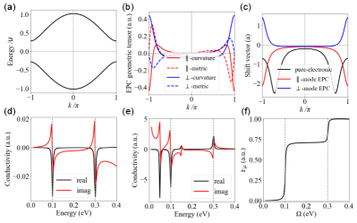
Using the representative parameters and band structure shown in Fig. 13(a), we numerically solve the EPC quantum geometric tensor and shift vectors as shown in Fig. 13(b,c). The results reveal that the EPC quantum metric and Berry curvature exhibit odd and even parity with respect to , respectively. The EPC shift vectors are found to be comparable in magnitude to pure-electronic shift vectors, indicating significant geometric contributions from EPC. The Ph-LO and second-order Ph-SHG conductivities are shown in Fig. 13(d) and (e), respectively, where phonon resonances appear as sub-gap peaks (i.e., photon energy below the electronic energy gap 0.57 eV), which agrees with the experimental observations [11]. In the static limit, as , the Ph-LO vanishes, while the imaginary component of Ph-SHG has a divergent response, aligning with the analytical discussions in Sec. LABEL:SM-sec:static_limit of Ref [50]. Note that the conductivity scales with the square of EPC strength . The integral function of Ph-LO conductivity, , as defined in Eq. 78, is shown in Fig. 13(f), with two step-wise values that correspond to the EPC character number of - and -mode, respectively.
The EPC topology can be discerned in the cases of band crossing with . From Eq. 57 and Eq. 84, the EPC character number for the -mode is calculated as:
| (90) | ||||
Non-zero contributions arise exclusively from the band-crossing states at . In the vicinity of , we find that , leading to:
| (91) | ||||
The character number, though not an integer, is protected by the singularity of the EPC Berry curvature at the band crossing, making it a topological quantity that remains robust under weak external perturbations.
VII Discussion
As discussed in Sec. IV.3, materials with strong EPC, such as Ca3Ru2O7 [60], BiTlSe2 [61], and ferroelectric materials like BaTiO3 [11, 46], are expected to generate strong Ph-LO and Ph-NLO signals, making them suitable for experimental observation. Two-dimensional ferroelectric materials with strong EPC are also particularly promising. Notably, EPC-modulated band crossings in Ca3Ru2O7 and BiTlSe2, as discussed in Sec. V.2 and demonstrated in Sec. VI, suggest the existence of topologically nontrivial EPC. This behavior, characterized using Eq.78, resembles band crossings in Weyl semimetals [48, 62, 63], albeit in a dynamic context [48, 62, 63]. This underscores the distinct topology of EPC, which resides in a Hilbert space different from that of pure-electronic systems.
To estimate the magnitude of Ph-NLO responses with the two-band approximation, the resonant strength of Ph-SC, denoted as , can be evaluated as:
| (92) | ||||
where is the line-width of -mode phonon. For comparison, the resonant strength of pure-electronic second-order NLO response is given by [48]:
| (93) |
where is the electron line-width. In the second-order Ph-NLO response, the transition dipole moment and the shift vector term are weighted by EPC matrix elements. A rough estimation based on GaAs [64, 65, 66, 67] suggests that , , . Consequently, the phonon-resonance peak of the second-order Ph-NLO response can achieve a comparable magnitude to that of the pure-electron second-order NLO response (on the order of ), and may even surpass it. This estimation is consistent with experimental observations [11].
In this work, several key approximations are adopted to simplify the analysis of electron-phonon and electron-photon interactions. Firstly, we treat the light field classically and consider the long-wavelength limit. The Born-Oppenheimer approximation, which assumes that electron dynamics are much faster than phonon dynamics, allows us to consider the electronic system in equilibrium with respect to phonon displacements. This holds for semiconductors with photon energies far from electronic resonance, where no real electron-hole pairs are generated. Additionally, phonon-coupled high-harmonic generation has been explored as a means of investigating nonadiabatic EPC [68]. Furthermore, by limiting the analysis to first-order electron-phonon coupling, we maintain accuracy under the assumption of a harmonic phonon system with weak perturbations. However, this approximation may break down in the presence of significant phonon anharmonicity or large phonon displacements, where higher-order interactions become important. Finally, the use of perturbative methods for both electron-phonon and electron-photon interactions is suitable for understanding the intrinsic material response, though nonperturbative effects such as polaron and polariton formation would require more complex treatment. These approximations set a foundational framework for analyzing Ph-NLO and quantum geometry, while also recognizing the limitations when extended to non-perturbative regimes. Future research could explore several extensions beyond these constraints. For instance, multi-phonon mediation, which involves multiple EPC matrix elements, could become significant for small-gap materials, extending the current single-phonon approach. Additionally, while this work emphasizes single-photon emission, multi-photon processes play a crucial role in applications like solar cells and optogenetics, warranting further investigation. Another potential extension involves open-ending phonon propagation, which we omit in favor of phononic Green’s functions connected to EPC matrix elements, ignoring net phonon excitations. This could lead to more complex phenomena such as the stimulated Raman effect. Additionally, while our current analysis focuses on monochromatic light and infinite illumination time to examine spatially uniform nonlinear optical (NLO) responses, it could be beneficial to expand this framework to account for the conditions of finite-duration light pulses used in experimental setups, as well as spatially dispersive effects [69].
Despite these limitations, the framework developed here provides a comprehensive foundation for understanding fundamental Ph-NLO responses and EPC quantum geometry.
VIII Conclusion
In this paper, we investigate the Ph-NLO responses through a systematic Feynman diagram approach. We examine both shift and ballistic mechanisms for indirect electron-photon interactions mediated by EPC. General expressions for Ph-NLO conductivities are derived up to the second order of photon perturbation, with particular emphasis on Ph-SC and Ph-SHG as notable cases. These novel EPC induced optical effects exhibit resonant responses below the electronic band gap, highlighting potential applications in terahertz photodetector and solar energy conversion technologies.
Furthermore, we propose a quantum geometric interpretation of the Ph-NLO response through a comprehensive analysis. We unveil the EPC matrix elements associated with inter-band EPC Berry connection, drawing an analogy to the matrix elements of the position operator related to pure-electronic Berry connections. Within the framework of complex Riemannian geometry, we identify the EPC Berry curvature and EPC quantum metric as key components governing phonon-induced polarization and velocity, respectively. In the context of noncentrosymmetric shift geometry, we obtain the EPC shift vector in analogy with pure-electronic shift vector. These newly introduced geometric quantities involve the phase properties of EPC, thereby expanding the framework of quantum geometry from the conventional pure-electronic Hilbert space (typically parameterized by electronic wave vectors) to the EPC Hilbert space, which is parameterized by phonon displacements and electronic wave vectors. This extension provides a comprehensive geometric explanation of the physical mechanisms underlying Ph-NLO responses. Moreover, we demonstrate the efficacy of Ph-NLO responses in probing the geometric aspects of EPC, and apply this approach to a general Rice-Mele model. Our work establishes a thorough foundation that integrates EPC, nonlinear optics, and quantum geometry.


Acknowledgements.
The authors thank insightful discussions with Mr. Zhichao Guo and Dr. Zhuocheng Lu in the Department of Physics, Zhejiang University. The work of J.H and W.L. is supported by the National Natural Science Foundation of China (NSFC) under Project No. 62374136. H.W. acknowledges the support from the NSFC under Grant No. 12304049 and Grant No. 12474240. K. C. acknowledges the support from the Strategic Priority Research Program of the Chinese Academy of Sciences (Grants Nos. XDB28000000 and XDB0460000), the NSFC under Grant No. 92265203, and the Innovation Program for Quantum Science and Technology under Grant No. 2024ZD0300104. W.L. also acknowledges the support by the Research Center for Industries of the Future at Westlake University under Award No. WU2022C041.Appendix A EPC geometry
To investigate the quantum geometric effect, we can reformulate the formula of EPC matrix element. Consider the electronic Hamiltonian as a function of crystal configuration, i.e. the function of ionic positions , with ranging over ionic sites and for unit cells. The -mode phonon vibration displaces the ionic positions as . Here is the eigen-vector of -mode vibration, which is dimensionless and normalized, reflecting the relative displacement strength of -th ion in -th unit cell. is a scalar in length dimension, scales the total vibration amplitude. In this case the EPC operator is defined as
| (94) |
where is the displacement quantum of the -mode phonon. refers to a mass constant. For notation simplicity we denoted . Using this notation, the EPC matrix element between states is written as . This can be further reformulated using the relation:
| (95) | ||||
which, when multiplied by , yields:
| (96) |
so that the intra-band term becomes:
| (97) |
which aligns with the Hellmann-Feynman theorem, stating that the first-order derivative of a Hamiltonian’s eigenvalues with respect to any parameter is given by the expectation value of the Hamiltonian’s derivative. The inter-band term is:
| (98) |
which takes the form of transition dipole moment, as discussed in Sec. V.1.
Appendix B Symmetry analysis
The time reversal symmetry operation acts to elementary matrix elements as:
| (99) | ||||
which leads to a key difference between pure-electronic and EPC quantum geometric tensors (Eq. 52 and 55) as:
| (100) | ||||
In systems preserving time-reversal symmetry, the EPC Berry curvature is an even function of while the pure-electronic Berry curvature is an odd function. Therefore, the EPC character number defined in Eq. 57 remains finite, while the Chern number defined in Eq. 58 vanishes, suggesting the essential distinction between pure-electronic and EPC quantum geometry. Both the pure-electronic and EPC shift vectors defined in Eq. 70 and 72 are unaffected by time-reversal symmetry operation:
| (101) | ||||
Therefore, non-zero diagram components , , and do not need time-reversal symmetry breaking, as do the Ph-NLO responses derived in Sec. IV.
The parity/inversion symmetry transformation , which flips spatial coordinates, we obtain:
| (102) | ||||
and the quantum geometric quantities transform accordingly:
| (103) | ||||
In centrosymmetric materials, the first-order diagram components do not vanish, while the second-order components become zero, as do the second-order Ph-NLO responses (Eq. 46 to 47), which is consistent with the general principle governing even-order nonlinear optics. If both and symmetries are preserved, we have , causing the EPC quantum metric to vanish.
Appendix C Expanded diagrams
References
- Bloembergen [1992] N. Bloembergen, Nonlinear optics: past, present and future, in Guided wave nonlinear optics, edited by D. B. Ostrowsky and R. Reinisch (Springer Netherlands, Dordrecht, 1992) pp. 1–9.
- Noffsinger et al. [2012] J. Noffsinger, E. Kioupakis, C. G. Van de Walle, S. G. Louie, and M. L. Cohen, Phonon-assisted optical absorption in silicon from first principles, Physical Review Letters 108, 167402 (2012).
- Thomson et al. [2013] R. Thomson, C. Leburn, D. Reid, et al., Ultrafast nonlinear optics (Springer, 2013).
- von Baltz and Kraut [1981a] R. von Baltz and W. Kraut, Theory of the bulk photovoltaic effect in pure crystals, Physical Review B 23, 5590 (1981a).
- von Baltz and Kraut [1981b] R. von Baltz and W. Kraut, Theory of the bulk photovoltaic effect in pure crystals, Physical Review B 23, 5590 (1981b).
- Belinicher and Sturman [1980] V. I. Belinicher and B. I. Sturman, The photogalvanic effect in media lacking a center of symmetry, Soviet Physics Uspekhi 23, 199 (1980).
- Tolles et al. [1977] W. M. Tolles, J. W. Nibler, J. R. McDonald, and A. B. Harvey, A review of the theory and application of coherent anti-stokes raman spectroscopy, Applied Spectroscopy 31, 253 (1977).
- Kwiat et al. [1999] P. G. Kwiat, E. Waks, A. G. White, I. Appelbaum, and P. H. Eberhard, Ultrabright source of polarization-entangled photons, Physical Review A 60, R773 (1999).
- Monserrat et al. [2018] B. Monserrat, C. E. Dreyer, and K. M. Rabe, Phonon-assisted optical absorption in BaSnO3 from first principles, Physical Review B 97, 104310 (2018).
- Dai et al. [2021] Z. Dai, A. M. Schankler, L. Gao, L. Z. Tan, and A. M. Rappe, Phonon-assisted ballistic current from first-principles calculations, Physical Review Letters 126, 177403 (2021).
- Okamura et al. [2022] Y. Okamura, T. Morimoto, N. Ogawa, Y. Kaneko, G.-Y. Guo, M. Nakamura, M. Kawasaki, N. Nagaosa, Y. Tokura, and Y. Takahashi, Photovoltaic effect by soft phonon excitation, Proceedings of the National Academy of Sciences 119, e2122313119 (2022).
- Gu et al. [2024] J. Gu, Y. Mou, J. Ma, H. Chen, C. Zhang, Y. Wang, J. Wang, H. Guo, W. Shi, X. Yuan, et al., Acousto-drag photovoltaic effect by piezoelectric integration of two-dimensional semiconductors, Nano Letters 24, 10322 (2024).
- Ahn et al. [2022] J. Ahn, G.-Y. Guo, N. Nagaosa, and A. Vishwanath, Riemannian geometry of resonant optical responses, Nature Physics 18, 290 (2022).
- Holder et al. [2020] T. Holder, D. Kaplan, and B. Yan, Consequences of time-reversal-symmetry breaking in the light-matter interaction: Berry curvature, quantum metric, and adiabatic motion, Physical Review Research 2, 033100 (2020).
- Resta [2011] R. Resta, The insulating state of matter: a geometrical theory, The European Physical Journal B 79, 121 (2011).
- Lai et al. [2021] S. Lai, H. Liu, Z. Zhang, J. Zhao, X. Feng, N. Wang, C. Tang, Y. Liu, K. S. Novoselov, S. A. Yang, et al., Third-order nonlinear Hall effect induced by the Berry-connection polarizability tensor, Nature Nanotechnology 16, 869 (2021).
- Sundaram and Niu [1999] G. Sundaram and Q. Niu, Wave-packet dynamics in slowly perturbed crystals: gradient corrections and Berry-phase effects, Physical Review B 59, 14915 (1999).
- Xiao et al. [2010] D. Xiao, M.-C. Chang, and Q. Niu, Berry phase effects on electronic properties, Reviews of Modern Physics 82, 1959 (2010).
- Nagaosa et al. [2010] N. Nagaosa, J. Sinova, S. Onoda, A. H. MacDonald, and N. P. Ong, Anomalous Hall effect, Reviews of Modern Physics 82, 1539 (2010).
- Gao et al. [2014] Y. Gao, S. A. Yang, and Q. Niu, Field induced positional shift of Bloch electrons and its dynamical implications, Physical Review Letters 112, 166601 (2014).
- Thouless et al. [1982] D. J. Thouless, M. Kohmoto, M. P. Nightingale, and M. den Nijs, Quantized Hall conductance in a two-dimensional periodic potential, Physical Review Letters 49, 405 (1982).
- Sodemann and Fu [2015] I. Sodemann and L. Fu, Quantum nonlinear Hall effect induced by Berry curvature dipole in time-reversal invariant materials, Physical Review Letters 115, 216806 (2015).
- Moore and Orenstein [2010] J. E. Moore and J. Orenstein, Confinement-induced Berry phase and helicity-dependent photocurrents, Physical Review Letters 105, 026805 (2010).
- Gao et al. [2023] A. Gao, Y.-F. Liu, J.-X. Qiu, B. Ghosh, T. V. Trevisan, Y. Onishi, C. Hu, T. Qian, H.-J. Tien, S.-W. Chen, et al., Quantum metric nonlinear Hall effect in a topological antiferromagnetic heterostructure, Science 381, 181 (2023).
- Wang et al. [2022] H. Wang, X. Tang, H. Xu, J. Li, and X. Qian, Generalized Wilson loop method for nonlinear light-matter interaction, npj Quantum Materials 7, 61 (2022).
- Ahn et al. [2020] J. Ahn, G.-Y. Guo, and N. Nagaosa, Low-frequency divergence and quantum geometry of the bulk photovoltaic effect in topological semimetals, Physical Review X 10, 041041 (2020).
- Gao et al. [2020] Y. Gao, Y. Zhang, and D. Xiao, Tunable layer circular photogalvanic effect in twisted bilayers, Physical Review Letters 124, 077401 (2020).
- Bhalla et al. [2022] P. Bhalla, K. Das, D. Culcer, and A. Agarwal, Resonant second-harmonic generation as a probe of quantum geometry, Physical Review Letters 129, 227401 (2022).
- Yi et al. [2023] C.-R. Yi, J. Yu, H. Yuan, R.-H. Jiao, Y.-M. Yang, X. Jiang, J.-Y. Zhang, S. Chen, and J.-W. Pan, Extracting the quantum geometric tensor of an optical Raman lattice by Bloch-state tomography, Physical Review Research 5, L032016 (2023).
- Ren et al. [2021] J. Ren, Q. Liao, F. Li, Y. Li, O. Bleu, G. Malpuech, J. Yao, H. Fu, and D. Solnyshkov, Nontrivial band geometry in an optically active system, Nature Communications 12, 689 (2021).
- Mera and Mitscherling [2022] B. Mera and J. Mitscherling, Nontrivial quantum geometry of degenerate flat bands, Physical Review B 106, 165133 (2022).
- Morimoto and Nagaosa [2016] T. Morimoto and N. Nagaosa, Topological nature of nonlinear optical effects in solids, Science Advances 2, e1501524 (2016).
- Wu et al. [2017] L. Wu, S. Patankar, T. Morimoto, N. L. Nair, E. Thewalt, A. Little, J. G. Analytis, J. E. Moore, and J. Orenstein, Giant anisotropic nonlinear optical response in transition metal monopnictide Weyl semimetals, Nature Physics 13, 350 (2017).
- Young and Rappe [2012] S. M. Young and A. M. Rappe, First principles calculation of the shift current photovoltaic effect in ferroelectrics, Physical Review Letters 109, 116601 (2012).
- Morimoto and Nagaosa [2024] T. Morimoto and N. Nagaosa, Direct current generation by dielectric loss in ferroelectrics, Physical Review B 110, 045129 (2024).
- Sipe and Shkrebtii [2000] J. E. Sipe and A. I. Shkrebtii, Second-order optical response in semiconductors, Physical Review B 61, 5337 (2000).
- Wang and Qian [2019] H. Wang and X. Qian, Ferroicity-driven nonlinear photocurrent switching in time-reversal invariant ferroic materials, Science Advances 5, eaav9743 (2019).
- Shi and Song [2019] L.-k. Shi and J. C. W. Song, Shift vector as the geometric origin of beam shifts, Physical Review B 100, 201405 (2019).
- Qian et al. [2022] C. Qian, C. Yu, S. Jiang, T. Zhang, J. Gao, S. Shi, H. Pi, H. Weng, and R. Lu, Role of shift vector in high-harmonic generation from noncentrosymmetric topological insulators under strong laser fields, Physical Review X 12, 021030 (2022).
- Hatada et al. [2020] H. Hatada, M. Nakamura, M. Sotome, Y. Kaneko, N. Ogawa, T. Morimoto, Y. Tokura, and M. Kawasaki, Defect tolerant zero-bias topological photocurrent in a ferroelectric semiconductor, Proceedings of the National Academy of Sciences 117, 20411 (2020).
- Tan et al. [2016] L. Z. Tan, F. Zheng, S. M. Young, F. Wang, S. Liu, and A. M. Rappe, Shift current bulk photovoltaic effect in polar materials—hybrid and oxide perovskites and beyond, npj Computational Materials 2, 1 (2016).
- Ogawa et al. [2017] N. Ogawa, M. Sotome, Y. Kaneko, M. Ogino, and Y. Tokura, Shift current in the ferroelectric semiconductor SbSi, Physical Review B 96, 241203 (2017).
- Cook et al. [2017] A. M. Cook, B. M. Fregoso, F. De Juan, S. Coh, and J. E. Moore, Design principles for shift current photovoltaics, Nature Communications 8, 14176 (2017).
- Yu et al. [2024] J. Yu, C. J. Ciccarino, R. Bianco, I. Errea, P. Narang, and B. A. Bernevig, Non-trivial quantum geometry and the strength of electron-phonon coupling, Nature Physics 20, 1 (2024).
- Ying and Law [2024] X. Ying and K. T. Law, Flat band excitons and quantum metric (2024), arXiv:2407.00325 [cond-mat.mes-hall] .
- Fei et al. [2020] R. Fei, L. Z. Tan, and A. M. Rappe, Shift-current bulk photovoltaic effect influenced by quasiparticle and exciton, Physical Review B 101, 045104 (2020).
- Onishi et al. [2022] Y. Onishi, T. Morimoto, and N. Nagaosa, Theory of shift heat current and its application to electron-phonon coupled systems, Physical Review B 106, 085202 (2022).
- Parker et al. [2019] D. E. Parker, T. Morimoto, J. Orenstein, and J. E. Moore, Diagrammatic approach to nonlinear optical response with application to Weyl semimetals, Physical Review B 99, 045121 (2019).
- Ortiz and Martin [1994] G. Ortiz and R. M. Martin, Macroscopic polarization as a geometric quantum phase: many-body formulation, Physical Review B 49, 14202 (1994).
- [50] Supplemental materials, where calculation details and related discussions are attached., Supplemental materials .
- Tiwari et al. [2024] S. Tiwari, E. Kioupakis, J. Menendez, and F. Giustino, Unified theory of optical absorption and luminescence including both direct and phonon-assisted processes, Physical Review B 109, 195127 (2024).
- Kioupakis et al. [2010] E. Kioupakis, P. Rinke, A. Schleife, F. Bechstedt, and C. G. Van de Walle, Free-carrier absorption in nitrides from first principles, Physical Review B 81, 241201 (2010).
- Noblet et al. [2021] T. Noblet, B. Busson, and C. Humbert, Diagrammatic theory of linear and nonlinear optics for composite systems, Physical Review A 104, 063504 (2021).
- Saparov et al. [2022] D. Saparov, B. Xiong, Y. Ren, and Q. Niu, Lattice dynamics with molecular Berry curvature: chiral optical phonons, Physical Review B 105, 064303 (2022).
- Im et al. [2022] J. Im, C. H. Kim, and H. Jin, Ferroelectricity-driven phonon Berry curvature and nonlinear phonon Hall transports, Nano Letters 22, 8281 (2022).
- Vanderbilt and King-Smith [1993] D. Vanderbilt and R. D. King-Smith, Electric polarization as a bulk quantity and its relation to surface charge, Physical Review B 48, 4442 (1993).
- Onoda et al. [2004] S. Onoda, S. Murakami, and N. Nagaosa, Topological nature of polarization and charge pumping in ferroelectrics, Physical Review Letters 93, 167602 (2004).
- Wang and Chang [2024] H. Wang and K. Chang, Geodesic nature and quantization of shift vector (2024), arXiv:2405.13355 [cond-mat.mtrl-sci] .
- Zhu and Alexandradinata [2024] P. Zhu and A. Alexandradinata, Anomalous shift and optical vorticity in the steady photovoltaic current, Physical Review B 110, 115108 (2024).
- Lihm and Park [2020] J.-M. Lihm and C.-H. Park, Phonon-induced renormalization of electron wave functions, Physical Review B 101, 121102 (2020).
- Wang et al. [2023] H. Wang, Y. Xiong, H. Padma, Y. Wang, Z. Wang, R. Claes, G. Brunin, L. Min, R. Zu, M. T. Wetherington, et al., Strong electron-phonon coupling driven pseudogap modulation and density-wave fluctuations in a correlated polar metal, Nature Communications 14, 5769 (2023).
- Chan et al. [2017] C.-K. Chan, N. H. Lindner, G. Refael, and P. A. Lee, Photocurrents in Weyl semimetals, Physical Review B 95, 041104 (2017).
- De Juan et al. [2017] F. De Juan, A. G. Grushin, T. Morimoto, and J. E. Moore, Quantized circular photogalvanic effect in Weyl semimetals, Nature Communications 8, 15995 (2017).
- Krotkus et al. [1995] A. Krotkus, S. Marcinkevicius, J. Jasinski, M. Kaminska, H. H. Tan, and C. Jagadish, Picosecond carrier lifetime in GaAs implanted with high doses of as ions: an alternative material to low-temperature GaAs for optoelectronic applications, Applied Physics Letters 66, 3304 (1995).
- Mattos et al. [1973] J. C. V. Mattos, W. O. N. Guimarães, and R. C. C. Leite, Photoexcited hot phonons and phonon lifetimes in GaAs, Optics Communications 8, 73 (1973).
- Strauch and Dorner [1990] D. Strauch and B. Dorner, Phonon dispersion in GaAs, Journal of Physics: Condensed Matter 2, 1457 (1990).
- Sjakste et al. [2015] J. Sjakste, N. Vast, M. Calandra, and F. R. A. N. C. E. S. C. O. Mauri, Wannier interpolation of the electron-phonon matrix elements in polar semiconductors: polar-optical coupling in GaAs, Physical Review B 92, 054307 (2015).
- Hu et al. [2024] S.-Q. Hu, H. Zhao, X.-B. Liu, Q. Chen, D.-Q. Chen, X.-Y. Zhang, and S. Meng, Phonon-coupled high-harmonic generation for exploring nonadiabatic electron-phonon interactions, Physical Review Letters 133, 156901 (2024).
- Gassner and Mele [2023] S. Gassner and E. J. Mele, Regularized lattice theory for spatially dispersive nonlinear optical conductivities, Physical Review B 108, 085403 (2023).