Phenomenology of Strong Interactions — Towards an Effective Theory for Low Energy QCD
Abstract
In this paper, we develop models applicable to phenomenological particle physics by using the string analogy of particles. These theories can be used to investigate the phenomenology of confinement, deconfinement, chiral condensate, QGP phase transitions, and even the evolution of the early universe. Other confining properties such as scalar glueball mass, gluon mass, glueball-meson mixing states, QCD vacuum, and color superconductivity can also be investigated in these model frameworks. We use one of the models to describe the phenomenon of color confinement among glueballs at the end of the paper. The models are built based on the Dirac-Born-Infeld (DBI) action modified for open strings with their endpoints on a D-brane or brane-anti-brane at a tachyonic vacuum.
I Introduction
String theory was conceived in the late 1960s to provide an explanation for the behavior of nuclear matter such as protons and neutrons Schwarz ; Schwarz1 . Even though the theory was not successful in explaining the characteristics of quarks and gluons at its inception, it promised an interesting intervention in other areas of physics Green ; Polchinski2 ; Johnson ; Zwiebach1 ; Becker . It showed capability in giving an insight into cosmology, astrophysics, and unification of the fundamental forces of nature which has been on the table of physicists for some time now. Consequently, the theory of Quantum Chromodynamics (QCD) was developed in the early 1970s to give a comprehensive explanation of nuclear matter Gross ; Politzer . The QCD theory is now accepted as the standard theory for strong interactions. Interestingly, recent development shows that string theory and QCD describe the same physics.
The formulation of Quantum Electrodynamics (QED) and QCD are almost the same. They are both formulated from field theory based on gauge theory which forms the foundation of the highly acceptable Standard Model (SM). The fundamental particles of these theories are studied based on the gauge boson they interchange: Photons for electrodynamic force, and bosons for electroweak force and gluon for strong nuclear force Quigg ; Collins1 ; Shaw . Subsequently, gravitational force does not fall under this category, so they are investigated under Einstein’s general theory of relativity. Physicists have bunged their hope on string theory to unify all the fundamental forces, this will fall under ’physics beyond the SM’ Aharony ; Maldacena ; Grana ; Polchinski3 ; Haro . Upon the similarities, quarks and gluons are color particles classified under three conventional colors (red, blue, and green) whilst photons are color neural bosons that mediate electrically charged leptons. Also, gluons self-interact due to their color charges but photons do not Quigg ; Collins1 .
Additionally, QCD falls short in explaining color-neutral particles such as bound states of gluons (glueballs) and quarks (hadrons and mesons), so string theory can be resorted for further description. The string-like description of hadrons arising from the quark model Amsler is an important phenomenon in applying string theory. Under this picture, when a quark and an antiquark are pulled apart, they behave as if they are connected by a rubber band (gluon) which becomes increasingly difficult to separate when the separation distance between them keeps increasing. This analogy gradually fails when the particles are brought closer and closer together. In this regime string theory fails and QCD theory becomes viable. Now, looking at the particles in terms of fundamental strings, string theory describes hadrons quite well and provides the background for the unification of the fundamental forces. In string theory, the strings are treated as particles, where different particles are associated with different string oscillations. The masses of the particles are also associated with the energy of the oscillating string. The intrinsic spin of the particle is associated with the two perpendicular oscillations of the string with its endpoints fixed on D-branes, similar to the direction of electric and magnetic fields in a photon. Hence, photons and gluons can be identified in terms of the open strings as spin-1 particles. The clockwise and anti-clockwise movement of the closed strings makes it possible to classify it among spin-2 bosons such as graviton. Since, QCD involves color fields, to study it under string theory we assume that the endpoints of the open strings on a D-brane serve as the source and sink of the color charge Bigazzi .
It has been conjectured that open bosonic strings studied at a tachyonic vacuum behave as if they are closed strings with no D-branes. However, soliton solutions in this region point to the presence of lower dimensional branes Sent2 ; Bardakci . This projection is also corroborated in superstring theories Sent1 ; Sen1 and evident in the first Recknagel ; Sen2 ; Harvey and second Kostelecky ; Sen ; Zwiebach2 ; Kostelecky1 ; Berkovits ; Harvey1 ; Gopakumar ; Gerasimov quantizations in string theories Sent4 . At the tachyonic vacuum, the negative energy density of the tachyons in the vacuum exactly cancels Witten1 the energy density of the D-branes i.e. . In non-BPS D-branes where is the D-brane tension Lindstrom ; Gustafsson ; Sent3 . It should be noted that at the total energy density of the tachyons and the brane tension vanishes identically, signifying the absence of open strings at that point. In this view, at a tachyonic vacuum, there will be no physical open string excitations because there are no D-branes. On the contrary, the ’usual’ field theory gives an alternative explanation, because shifting the vacuum and expanding around its ’true’ minimum can change a negative square mass of the tachyons to a positive one even though it does not completely remove all the states. Since it will not cost any energy to adjust the fundamental strings on the worldvolme of the D-branes at a tachyonic vacuum, it will be difficult to notice their presence. Hence, fluctuations around the vacuum represent the presence of lower dimensional D-branes Sent2 ; Bardakci . These phenomena have been investigated in references Sen ; Zwiebach2 ; Kostelecky using open string field theory Witten2 .
In this paper, we modify the Dirac-Born-Infeld (DBI) action, so that the associated open strings with their endpoints on the remaining lower-dimensional branes at the tachyonic vacuum can be analyzed. The objective is to develop models that can mimic QCD theory both in the UV and IR regions with UV safety. The models can be applied in developing potential models such as the linear confining and Cornell potential models. In the analysis, we consider that the string worldsheet falls inside the D-brane worldvolume making it easy for the endpoints of the strings to be connected by the flux line on the worldvolume to form a close string suitable for modeling color confinement in a flux-tube like picture. The dynamics of the strings tangential to the D-brane worldvolume is represented by the gauge field and the component transverse to the worldvolume is represented by a massless scalar field . The net flux involved is determined by the source and sink of the flux carried by the endpoints of the string on the lower dimensional remnants of the original D-brane in the vacuum. Also, the condition for minimum energy warrants that the flux does not spread because the source and sink of the flux emanate from a pointlike object on the D-brane worldvolume.
The paper is organized as follows: In Sec. II we review Tachyons and D-branes, divided into two subsections, under Sec. II.1 we review Tachyons, and in Sec. II.2 we review D-branes. We present the Modification of the Dirac-Born-Infeld Action which serves as the bases for the study in Sec. III. Also, in subsection III.1 we review the Dimensional Reduced Yang-Mills theory and its intended consequences in relation to the Standard Model (SM) of Particle Physics. Section IV and subsequent sections contain our original contributions to the subject. We present the Bosonic String at Tachyonic Vacuum in Sec. IV, where we present the details of dimensional reduction from Dirac-Born-Infeld action to conducive for describing SM particles. We present Gauge Theories Modified with , in Sec. V, this section was divided into two. We studied Fermions Coupled to Fundamental Strings at Tachyonic Vacuum in Sec. V.1 and Non-Abelian Gauge Theory in Sec. V.2. Section VI contains the Phenomenon of Gluon Confinement, divided into four subsections. We present The Model in Sec. VI.1, Confining Potentials in Sec. VI.2, Gluon Condensation in Sec. VI.3 and strong Running Coupling and QCD -function in Sec. VI.4. we present our findings and Conclusions in Sec. VII.
II Review of Tachyons and D-branes
II.1 Tachyons
Generally, tachyons are classified as particles that travel faster than light or weakly interacting superluminal particles. Relativistically, single particle energy is expressed as , where is the spatial momentum and is the mass of the particle. For a particle to be faster than light, the relativistic velocity . Hence, for tachyons with real , must necessarily be imaginary Bilaniuk . However, this analogy does not make a strong and convincing case for the tachyons. Rather, Quantum Field Theory (QFT) provides some satisfactory explanation to the dynamics of tachyons. QFT suggests that particles that travel faster than light does not exist in nature. So tachyons are simply unstable particles that decay. Based on this understanding, we consider a scalar field, say , with the usual kinetic term and a potential whose extremum is at the origin. If one carries out perturbation quantization about up to the quadratic term and ignores the higher order terms in the action, we obtain a particle-like state at . These results have two interesting interpretations; if we have a particle of mass but for we have a tachyonic state with a negative . In this case, tachyons can be given a physical meaning. So far, we know that the tachyons have negative and potential whose maximum is at the origin, thus a small displacement of at the origin will cause it to grow exponentially with time towards the true minimum. By the above description, tachyons can be represented by a potential such as
| (1) |
where are constants. Hence, tachyonic fields are associated with the ’usual’ Higgs fields where the Higgs particles acquire negative square mass at the true minimum of their potential. Accordingly, tachyons in QFT are related to instability that breaks down the perturbation theory in normal field theory. The usual quantization where the cubic and higher order terms are considered small corrections to the quadratic term is no longer tenable. Since has its maximum at , it renders it classically unstable at that point. So one cannot guarantee that the fluctuation at that point is small. This behavior comes with an inbuilt solution i.e. one can expand the potential about the true minima up to the quadratic term and proceed with the perturbation quantization about that point. Thus, the cubic and higher-order terms in the expansion can be discarded. This process will lead to the creation of a particle with a positive mass in the spectrum. This process removes the tachyonic modes in the spectrum. Additionally, in D-brane systems, the theory must be invariant under symmetry, i.e. and in the presence of brane-anti-brane, the theory must necessarily be invariant under phase symmetry . Indeed, there are some benefits in working in tachyonic modes otherwise we can define a new field, , and express the potential in terms of the new field,
| (2) |
Working with this potential from the onset will remove the tachyonic mode from the spectrum because will be positive. However, there are some benefits to working with tachyonic fields, for instance, they possess high symmetry. This symmetry might not be explicit in as it is in . The high symmetry in tachyonic fields leads to the phenomenon of spontaneous symmetry breaking, where the potential has more than one minima i.e. corresponding to . This phenomenon is well known in elementary particle physics Sent3 .
II.2 D-branes
Recent advances in string theory have provided some explanations regarding nonperturbative features of QCD theory, thanks to the discovery of D-branes. The study of D-branes gives insight into physically relevant systems such as black holes, supersymmetric gauge theories, and the connection between Yang-Mills theories and quantum gravity. Upon the numerous progress, a consistent nonperturbative background-independent construction of the theory is yet to be developed. This poses a challenge in directly addressing cosmological problems. There are five known ways for which supersymmetric closed strings can be quantized, i.e. IIA, IIB, I, heterotic and heterotic superstring theories. Individually, they give a perturbative description of quantum gravity. However, they are connected through duality symmetries Hull ; Witten . Indeed, some of these dualities are nonperturbative in nature because the string coupling in one theory may have an inverse relation with the other. The superstring theories together with M-theory (a theory that unifies superstring theories) consist of an extended object of higher dimensions, called D-branes. Each of these theories contains branes but in different complements. Particularly, IIA/IIB superstring theories consist of even/odd D-brane dimensional configurations. Using the appropriate duality transformations, one brane can be mapped onto the other even with the strings connecting them. Thus, none of the branes are seen to be more fundamental to others. This process is commonly referred to as ’brane democracy’.
Before moving into the specific kind of strings set out for this study, we will shed light on the features of open and closed strings. Closed strings are topologically the same as a circle , i.e. . They give rise to a massless set of spacetime fields, identified as graviton , dilaton , antisymmetric two-form and an infinite set of massive fields upon quantization. Supersymmetric closed strings are also related to massless fields identified with graviton supermultiplets such as Ramond-Ramond -form fields and gravitino . Consequently, the quantum theory of closed strings is naturally related to the theory of gravity in spacetime. On the other hand, open strings are topologically similar to the interval . They give rise to massless gauge field in spacetime upon quantization. Supersymmetric open strings are also associated with massless gaugino . Accordingly, open strings have their ends on Dirichlet -branes (D-brane) and the gauge field lives on the worldvolume of the D-brane. Upon these differences, the physics of closed and open strings are related at the quantum level. Closed strings were first observed through the one-loop process of an open string. Under this process, close strings appeared as poles in nonplanar one-loop open string diagrams Gross1 ; Lovelace . The open strings have their endpoints on the D-branes whilst close strings have no endpoints. The degree of freedom of the open strings is associated with standing wave modes on the fields while the close strings correspond to left-moving and right-moving waves. The boundary conditions for open strings on the bosonic field are Neumann (freely moving endpoints) and Dirichlet boundary conditions (fixed endpoints). The close string on the other hand corresponds to periodic and anti-periodic boundary conditions.
Some D-branes have unstable configurations both in the supersymmetric or the nonsupersymmetric string theories. The instability is attributed to tachyonic modes with negative square mass in the open string spectrum, we are interested in investigating the effects of the tachyonic modes Sen ; Zwiebach . Some D-brane configurations with open strings containing tachyons are:
Brane-antibrane; it is a type IIA or IIB string theory with parallel D-branes separated by ( is the string length scale). They also carry tachyons in their open string spectrum. The difference in their orientation leads to opposite Ramond-Ramond (R-R) charges Hughes . So the brane and anti-brane pair can annihilate leaving a neutral vacuum because the net R-R charge will be zero.
Wrong-dimension branes; the D-brane with wrong dimension for type IIA/IIB with odd/even spatial dimension for instead of even/odd dimensions carry no charges under classical IIA/IIB supergravity fields. They have tachyons in their open string spectrum. Such branes can annihilate to form a vacuum without violating charge conservation.
Bosonic D-branes; just as the wrong-dimension branes of type IIA/IIB string theory, the D-brane of any particular dimension in the bosonic string theory have no conserve charge and has tachyons in their open string spectrum. Also, they can annihilate to form a neutral vacuum without violating charge conservation.
III Modification of Dirac-Born-Infeld Action
We begin the study with the Born-Infeld action (BI) Born sometimes referred to as Dirac-Born-Infeld action (DBI) Gibbons ; Dirac . The focus will be on D-branes Polchinski ; Taylora which are nonperturbative states on which open strings live. They are equally coupled with closed strings, Ramond-Ramond states and other massive fields. The nonperturbative nature of the action makes it possible to describe low energy degrees of freedom of the D-branes Leigh making it possible for application in low energy QCD. The distinction between the DBI action, other -branes and supermembrane theories Hughes ; Bergshoeff ; Townsend is the presence of gauge field in the worldvolume of DBI. The gauge field is associated with virtual open string states. Consequently, we obtain confinement of the fundamental strings with their endpoints fixed on the branes. Generally, the action can be expressed as
| (3) |
where , and are the induced metric tensor, antisymmetric tensor, and dilaton field to the D-brane worldvolume respectively. Also, is the worldvolume electromagnetic field strength of and is a set of Chern-Simon terms while
| (4) |
is the brane tension and is the string coupling, with associated string tension
| (5) |
In type IIA/IIB string theory with even/odd are associated with quantum open strings containing massless and fields. These fields are the consequence of the gauge field living on the hypersurface and transverse excitations. The geometry of D-brane is not flat, so we generally define the embedding , where represent coordinates on the D-brane worldvolume , and is the ten functions mapping from onto the spacetime manifold . Introducing the scalar field into the action, it becomes invariant under diffeomorphism and Abelian gauge transformations. So, a way of fixing the freedom of the former is to adopt a ’static gauge’ such that
| (6) |
The remaining fields are
| (7) |
which are the transverse coordinates to the worldvolume Tseytlin ; Taylor ; Taylor1 where is a spatial dimension. Thus, one can choose for superstring theory and for bosonic string theory. Under this gauge, the originally -dimensional global poincaré symmetry spontaneously breaks down to a product of dimensional poincaré group with dimensional rotational symmetry group i.e. . For a D-brane possessing extends over -dimensional subspace of -dimensional space. The focus will be on a D-branes with -dimensional hyperplanes in -dimensional space. Again, according to the static gauge fixed above, there are two possible consistent truncations;
-
•
; corresponds to pure BI theory Born in and
-
•
; also corresponds to Dirac’s theory Dirac of minimal timelike submanifolds of .
We can introduce the transverse scalar fluctuations by defining the induced metric as
| (8) |
that will approximate the D-brane worldvolume to near flat. In this study, we are interested in understanding the dynamics of bosonic open strings with tachyonic modes in their spectrum, so we will proceed systematically toward that objective. The worldvolume theory of non-BPS D-brane in IIA/IIB string theory corresponds to a massless vector field, transverse oscillating scalar field and a tachyonic field Sent . Accordingly, the leading order of the action results in dimensional reduction -dimensional Yang-Mills theory. Besides, higher-order corrections, , to the order of the string scale are also possible. Since we are proceeding with the assumption that the massless fields are slowly varying compared to the string length , i.e. we discard the higher order derivatives and write the DBI action Leigh ; Garousi ; Callan in a simple form without the explicit presence of the tachyons. Therefore, Eq.(3) takes the form
| (9) |
Now we will express the extended form of the DBI by including the dynamics of the tachyons as studied in Garousi . Accordingly,
| (10) |
where is the tachyon potential and is, as usual, the kinetic energy of the tachyons Garousi1 . Under this conjuncture, the action vanishes at the minimum of the tachyon potential Sent2 ; Sent1 ; Recknagel . We will now continue the discussion by approximating that the D-branes are nearly flat, with constant dilaton, and vanishing antisymmetric two-form term to remove the close string quanta in the system.
III.1 Dimensional Reduction Yang-Mills Theory
Studying D-branes under Yang-Mills theory enables us to understand the physics of D-branes without necessarily applying any complex string theory artifacts. Detailed analyses show there is enough evidence that super Yang-Mills theory carries a lot of information concerning string theory than one may possibly imagine Banks . Besides, recent developments in high-energy physics investigations have shown that string theory gives insight into low-energy field theories in the nonperturbative region Taylor . This has been conjectured to be equivalent to QCD where confinement can be realized in color fluxtube picture. From Eq.(9), in the limit of vanishing and further assuming that the D-branes are almost flat, close to the hypersurface i.e. , . Again, we suppose that the fields are slowly varying such that and are in the same order. Therefore, the action can be expanded as
| (11) |
Here, is the -brane worldvolume and is the Yang-Mills coupling given by,
| (12) |
The second term in Eq.(11) corresponds to gauge theory in dimension coupled with scalar fields. Introducing fermions fields, as mentioned below Eq.(3) into the action, we recover the supersymmetric Yang-Mills theory in Super Yang-Mills action,
| (13) |
In the case of N parallel D-branes, the p-dimensional branes must be distinctively labeled from . Subsequently, the massless scalar fields living on the individual D-brane worldvolume are related to gauge group. The fields arising from the strings stretching from one brane to the other are labeled as , where specifies the individual branes that carry the endpoints of the strings. The strings are oriented such that they consist of fields, corresponding to individual fields. The mass of the strings is proportional to the separation distances between the branes. So the strings become massless Witten1 ; Taylora when the D-branes get very close to each other. Hence, the open strings can transform under the adjoint representation U(N). Thus, the corresponding fields can be decomposed similarly to adjoint supersymmetric gauge field in -dimensions. With the stacks of D-branes crossing each other at some angles, one can also break the U(N) symmetry into SM particle physics i.e. Lust . In sum, the DBI action can be generalized into a non-Abelian gauge group by considering stacks of D-branes instead of a D-brane.
A major motivation for string dual to QCD is derived from the ’t Hooft large -limit Hoofta2 ; Witten4 . Though, and have different representations, in the limit of , the difference can be overlooked. Thus, the number of gluons can be approximated as . This is more than the quark degree of freedom , therefore, we expect the dynamics of the gluons to dominate in this regime Mateos .
IV Bosonic Strings at Tachyonic Vacuum
Generally, there are two known boundary conditions associated with open strings. The Dirichlet (fixed) boundary condition is where the coordinates are normal to the brane, and under Neumann (free) boundary condition is where the coordinates are parallel to the brane Dai ; Leigh ; Polchinski1 . It has been established Callan1 that a small disturbance normal to the string and the brane are likely to reflect back with a phase shift of , corresponding to a Dirichlet boundary condition. Some study in this regard has been carried out in Rey ; Lee using Nambu-Goto action for strings with their endpoints on a supergravity background of D-branes. Since the strings attached to the -branes manifest themselves as electric charges, the Neumann boundary condition where the endpoints of the strings are freely oscillating will lead to the production of electromagnetic dipole radiation at the asymptotic outer area of the brane.
In this section, we will consider Eq.(10) which includes the dynamics of tachyons on open strings. Accordingly, we will keep all the arguments made for the -dimensional DBI action, but we will reduce the spacetime dimension from to . One of the major differences between superstring theory and particle theory is that the former lives on -dimensional spacetime and the latter on -dimensional spacetime. Nonetheless, this discrepancy can be dealt with using compactification scheme Gell-Mann ; Guendelman ; Randall , where the spacetime is divided into an external non-compact spacetime and an internal compact spacetime . We can combine these two phenomena into a single expression as
| (14) |
We adopt a physically realistic phenomenon where . Additionally, we can set a compact scale , where is the radius of the internally compact spacetime, smaller than the string mass Grana ; Shiraishi . As a result, the energy required for this work must lie in the range . So, the worldvolume coordinate becomes , where . Consequently, we will reduce the dimension to -dimension with metric signature. We will also decouple the available transverse fluctuating scalar fields and the antisymmetric tensor i.e., . Keeping the dilaton field constant, we get
| (15) |
In the above expression we calculate the determinant up to the second-order derivative discarding higher-order corrections. In view of field theory at tachyonic vacuum, the D-branes do not vanish completely rather, there are lower dimensional D-branes present. So, the endpoints of the strings sitting on the low dimensional D-branes behave like point-like particles which serve as the source and sink of the flux carrying the color particles. For instance, expanding around the ’true’ minimum of the potential gets rid of the tachyons leading to a particle with a positive square mass.
We consider a field configuration such that , in this case, the potential can be expressed as
| (16) |
so
| (17) |
As a result, the Lagrangian of the system becomes,
| (18) |
here, we have introduced a dimensionless quantity which will be referred to as a color dielectric function, subsequently. If we set the string tension becomes and Brito ; Adamu ; Issifu ; Issifu1 ; Issifu2 . It is important to mention at this point that the potential of the field, , follows the same discussion as contained in Sec. II.1. It has its minimum at , where is the ’true’ vacuum of the potential. To apply this theory to asymptotically free systems, the potential must satisfy additional conditions,
| (19) |
necessary for stabilizing its vacuum Rosina ; Adamu ; Kharzeev . These restrictions make it possible to apply Eq.(18) in investigating asymptotically free particles such as gluons in a QCD-like fashion. Here, the modified Abelian gauge mimics the role of the non-Abelian gauge in the ’usual’ QCD theory. We treat the endpoints of the open string on the lower dimensional branes as the source of quark and an anti-quark (if fermions are present) or valence gluons and the string connecting them as gluons that mediate the interactions. Also, the potential plays a similar role as a quantum correction in gluodynamics theory that breaks the conformal symmetry to bring about gluon condensation Kharzeev ; Gaete ; Issifu1 . This model has been used to study the color confinement of glueballs at a finite temperature in Ref.Issifu .
Considering brane-anti-brane systems, we note that the model must be invariant under the global rotation . This warrants an introduction of a complex scalar field with potential Sen3 . So, we can redefine the scalar field in a form,
| (20) |
to incorporate the D-brane and anti-D-brane dynamics. Supposing that the original gauge field is on the worldvolume of the D-brane represented by a complex scalar field , we will have a dual gauge field also on the wordvolume of the anti-D-brane represented by the conjugate field . Therefore, the string here has its endpoints on remnants of D-brane and the anti-D-brane parallel to each other. Imposing gauge invariance on the scalar sector, we can define an Abelian covariant derivative
| (21) |
where is a gauge field which is dual to . Accordingly, the Lagrangian in Eq.(18), can be extended as
| (22) |
where and are two independent Abelian field strengths. Aside from the original gauge invariance of the Lagrangian, it is also invariant under the gauge transformation,
| (23) |
This Lagrangian can undergo a spontaneous symmetry breaking (SSB) process (when we choose an appropriate potential) similar to the usual Abelian Higgs mechanism Quigg ; Collins1 . In this case, plays a role similar to the ’usual’ Higgs field in the standard model of particle physics. This process will also lead to the observation of Goldston boson (most likely due to the ) corresponding to the number of unbroken symmetries signaling confinement as well Issifu ; Nielsen . This model has been exploited in detail to study glueballs and color superconductivity in Issifu2 . It is important to mention that (22) is valid when we consider D-brane and an anti-D-brane system in the framework of DBI action Erkal ; Senn . It is suitable for describing massless particles such as glueballs or gluon confinement.
V Gauge Theories Modified with
V.1 Fermions Coupled To Fundamental Strings at Tachyonic Vacuum
In this section, we introduce Dirac’s Lagrangian for free particles adopted by Maxwell in the unification of electric and magnetic field interactions. We introduce the dynamics of the fermions which were dropped in the previous discussions as stated below Sec. III. However, it will be introduced here through Dirac’s equation modified by while taking into consideration all gauge invariance properties. We start with the well-known Dirac’s Lagrangian for free particles
| (24) |
Even though this Lagrangian is well known in QED, it is also used to describe free nucleons in terms of their composite fermions; protons, and neutrons in strong interaction. It is invariant under global phase rotation,
| (25) |
Noticing that the fields in the Lagrangian are color neutral in nature, to apply them in studying color particles such as the ones considered here, we need to modify the fields. Hence, we will modify the bispinors with the in order to give them some color features. Thus, we perform the transformations
| (26) |
where is a function therefore, the gradient in Dirac’s equation will transform as
| (27) |
and Lagrangian (24) becomes
| (28) |
The local gauge invariance is violated by and the gradient function . To ensure local gauge invariance is satisfied, we modify all variables involving derivatives, and color neutral fields such as the Dirac -matrix with and also introduce the electromagnetic field in other to make the equation gauge invariant. Consequently, we will adopt the transformations,
| (29) |
where is the gauge-covariant derivative and is the electric charge. This type of derivative corresponds to momentum transformation, . By this transformation, the gauge field also gets modified and enters the Lagrangian as . It also introduces a coupling between the electromagnetic field and matter in a form . So Eq.(V.1) becomes
| (30) |
consequently, the electromagnetic field transforms as
| (31) |
Equation (V.1) looks similar to Dirac’s Lagrangian with interaction term that couples the gauge field to the conserve current with a modified mass term . Also, becomes invariant under local phase rotation, granting interaction between , and with momentum . In this way, the Lagrangian has been modified, but we ensure that all conservation laws are duly respected.
Now, to derive a complete Lagrangian that can mimic QCD theory, we include the kinetic energy term of the gauge field which has been derived in Eq.(18), thus,
| (32) |
This expression looks similar to the usual QED Lagrangian with as intermediate field/particle and a mass term modified by color dielectric function, . As a result, this expression approximates the non-Abelian QCD theory with an Abelian one. This was motivated by the projection that the confining regime of QCD is mostly Abelian dominated Hoofta1 ; Ezawa ; Shiba ; Suzuki ; Sakumichi . The spinor fields and represent the quarks and antiquarks and the modified gauge field also describes gluons. All the long-distance behavior of the gluons is absorbed in . The observed mass of the system is expected to have a fixed value at the beginning of the interaction and at the end of the interaction , so it can be measured precisely. That is, the dielectric function should be such that , where is the energy at the beginning of the interaction and is the energy at the end of the interaction. Thus, is the constituent quark mass function of the system. We have presented a detailed study of this theory in Refs.Issifu1 ; Adamu
Since the renormalization theory remains the systematic approach for which UV divergences can be resolved Neubert , we will compare the result with the renormalized QED Lagrangian to properly identify the nature of the dielectric function in the context of renormalization factor , where is a scale that comes from the dimensional regularization scheme Bollini ; Hoofta . The objective is to ensure that the result obtained in Eq.(32) does not pose any UV divergences. When the real QED Lagrangian is written in terms of the renormalized factors, it takes the form,
| (33) |
where
| (34) |
the two equations bear some resemblance, so we can compare them. With the gluon propagator renormalization factor, the quark-quark-gluon vertex renormalization, and the quark self-energy renormalization factor. Additionally, the covariant derivative can be expressed in terms of the renormalized factors as , gauge invariance requires that . We have substituted the ’conventional’ representation of the renormalization factors and with and respectively, and to make the distinction more obvious relative to fermions and the gauge field. The renormalized fields are without subscript ’0’ Itzykson ; Pascual ; Peskin ; Collins ; Weinberg ; Weinberg1 ; Schwartz . Comparing the results in Eqs.(32) and (33), we identify and the gauge invariance warrant that, . Thus, in addition to the color properties carried by the color dielectric function, it also absorbs the UV divergences. Consequently, the dielectric function follows the restrictions,
| (35) |
From the gauge conditions adopted above, a gluon mass term,
| (36) |
will not be invariant under the local gauge transformation in Eq.(31) because
| (37) |
Consequently, local gauge invariance accounts for the existence of massless photons Quigg .
V.2 Non-Abelian Gauge Theory
In this section, we will focus on constructing a non-Abelian gauge theory traditionally used for describing the strong nuclear force. Additionally, we buy into the projection that proton and neutron have the same mass and are charge independent due to the strong nuclear force. Therefore, there is an agreement that isospin is conserved in strong interactions. As in the case of QED theory, we will base the discussions on -isospin gauge theory introduced by Yang and Mills Yang , elaborated by Shaw Shaw . Here, we will consider Eq.(24) as the Lagrangian for free nucleons with composite fermions, protons (p), and neutrons (n)
| (38) |
The Lagrangian is invariant under global spin rotation
| (39) |
also, isospin current, , is conserved therefore, proton and neutron can be treated symmetrically in the absence of electromagnetic interactions. In that case, the distinction between proton and neutron is arbitrary and conventional under this representation.
To maintain the differences between the Abelian theory treated in Sec. V.1 and the non-Abelian theory intended for this section, we will replace from the Abelian covariant derivative, , expressed in Eq.(29) with its non-Abelian counterpart i.e.,
| (40) |
We have also replaced with , the strong coupling constant to make the analysis distinct from Sec. V.1 and befitting for describing strong interactions. Despite the similar global gauge invariance satisfied by both theories, they also exhibit some major differences; the algebra of the non-Abelian group is more complex and the associated gauge bosons self-interact due to the structure of the non-Abelian group. Accordingly, the field can be expressed as,
| (41) |
where the three non-Abelian gauge fields are . The generators and ) are associated with Pauli’s matrices, are the charged gauge bosons and the isospin step-up and step-down operators exchange following the absorption of boson. The gradient in Eq.(24) will then transform as,
| (42) |
thus,
| (43) |
Again, following similar procedure as adopted for Eq.(V.1) using the necessary transformations, we obtain
| (44) |
with gauge invariant transformation similar to Eq.(31),
| (45) |
By comparing Eq.(V.2) and Eq.(45) we can deduce,
| (46) |
The -isospin generators can be expressed in terms of commutator relation,
| (47) |
Conventionally, do not commute with others in different spatial directions, so only one component can be measured at a time and this is taken to be the third component , generally in -direction.
We will now develop the field strength tensor that will form the kinetic term of the gauge field. Starting with the electromagnetism gauge, we can construct,
| (48) |
From these transformations, we can develop a gauge invariant field,
| (49) |
where the field strength tensor transforms under the dielectric function as
| (50) |
We know from the QED relation constructed in Sec. V.1 that the field strength can be expressed as
| (51) |
We adopted the expression for defined in Eq.(V.2), regrouping the terms in the above equation yields,
| (52) |
higher derivative terms were discarded. We can cast this result in a slightly symmetric form by using the identity , so
| (53) |
Using this identity appropriately leads to,
| (54) |
This equation shows the additional terms that come from the non-vanishing commutators due to the non-Abelian group structure. By this expression, we deduce that a term can be added to to modify to achieve the desired transformation property we require. With this inspiration, the observed electromagnetic field strength tensor can be modified to read,
| (55) |
Substituting the definition for in Eq.(29) into the above expression, we obtain
| (56) |
The commutator vanishes for Abelian theories. Applying this transformation to Eq.(50) yields,
| (57) |
Expanding the commutator using the transformation Eq.(V.2) to enable us to compare the outcome to the nonvanishing commutator relations in Eq.(V.2) leads to,
| (58) |
The commutator relations that come after the first term in the last step are the exact terms required to cancel the extra terms in Eq.(V.2). Therefore, the field strength tensor expressed in Eq.(57) has the required structure under local gauge transformation. Combining Eqs.(44) and (49) gives rise to modified Yang-Mills Lagrangian Quigg ; Yang ,
| (59) |
where is the modified nucleon mass. This Lagrangian is also invariant under local gauge transformations and does not permit the existence of mass term . It should also be noted that introducing the non-Abelian gauge leads to the automatic cancellation of the color dielectric function. Hence, we can infer that the color dielectric function attached to the Abelian gauge induces strong interaction properties. Using the expression in Eq.(41) and the commutator relation in Eq.(47), we can rewrite the transformed version of Eq.(57) as
| (60) |
in the last step we have dropped the three isospin generators of the gauge field because they are linearly independent. Generally, non-Abelian gauge groups that do not fall under , the Levi-Civitá symbol is replaced with the antisymmetric structure constant .
The introduction of the -isospin symmetry by Heisenberg Heisenberg preceded the development of the quark model. That notwithstanding, the only known fundamental components of the nucleon describing strong interactions are up-quark () and down-quark (). While the proton is composed of two -quarks and a -quark, the neutron is also composed of two -quarks and an -quark. Indeed, these particles remain the only known constituents of proton and neutron with almost the same mass and coupling force. Hence, Eq.(59) can be used to study the behavior of quarks and gluons inside hadrons. In that case, the up/down quarks are treated as having the same mass and -charge, so they are seen as similar particles with different isospin states, , same as the nucleon. Interestingly, the spin addition of the quark constituents of proton and neutron agree with and respectively. Similar to the isospin representation of the nucleon field in Eq.(38) the quark field can be represented as
| (61) |
Nevertheless, the mathematical structure of this theory is the same as QCD, the theory that describes the characteristics of quarks and gluons inside the hadrons.
Again, the strong interaction is well known for its invariance under quark color permutations, so we can express the quark wave function for color triplet representation as
| (62) |
where , and . This is invariant under transformation of the form
| (63) |
where are the eight phase angles and is a matrix representing eight independent traceless Hermitian generators of the group. Ignoring the differences in quark masses, it can also be applied in studying u, d and s quark systems,
| (64) |
The generators are fundamentally equivalent to Pauli’s matrices for the representation and they satisfy the Lie algebra,
| (65) |
similar to Eq.(47), is the structure constant. Consequently, to generalize the relation in Eq.(V.2) for QCD under the color symmetry, we substitute the antisymmetric tensor for the antisymmetric structure constant Collins1 .
Finally, the models exhibit the expected asymptotic free Gross ; Politzer behavior at high energy regions while at low energies color confinement and hadronization sets in. Here, represents constituent quark mass function Atkinson while is the bare quark mass. As analyzed in Sec. V.1, the constituent mass of the quarks in the asymptotically free region can be determined as , while the constituent mass at the nonperturbative (low energy) region where color confinement is expected, will be . Hence, it is possible to have the same constituent quark mass in both the UV () and the IR () regimes, if indeed the bare quark mass in both regimes are the same Adamu ; Eichten , because the behaves as, . However, there is evidence that is small in the IR regime and large in the UV regime Adamu ; Issifu1 . Accordingly, if we require color confinement in both regions, because higher bare quark mass is required to obtain confinement in the UV region than it is required in the IR region.
VI Phenomenology of Glueball Confinement
In this section we will use one of the models built in Sec. IV specifically, Eq.(18) to build a model that describes the features of confining glueballs. Apart from the insight into the behavior of the glueballs in both the IR and the UV regions, it will serve as a test to the models developed earlier. The model will be based on electric field confinement, commonly referred to as the chromoelectric flux confinement. In that light, we will define the indices of the gauge field such that the chromomagnetic flux is eliminated from the system (i.e. ) and only the static sector of the scalar field, i.e. , is available for analysis. This ensures that the color particles that generate the gluons are static. This section will enable us to see how the Abelian gauge can be used to approximate a non-Abelian theory. Additionally, the color dielectric function absorbs the long-distance dynamics of the gluons such that the photon propagator emanating from the Abelian gauge field does not decouple at longer wavelengths. We will further demonstrate that the is directly related to the QCD -function and the strong running coupling constantly.
VI.1 The Model
The equations of motion for Eq.(18) are,
| (66) |
and
| (67) |
Expressing the above equations in spherical coordinates,
| (68) |
where, (only electric field components are considered) and as discussed in Sec. IV. Accordingly,
| (69) |
where
| (70) |
and
| (71) |
is an integration constant, we also substituted to achieve the desired objective. Now we choose a potential that satisfies all the conditions expressed in Sec. IV thus,
| (72) |
where and are dimensionless constants, is the tachyon decay constant. This potential contains tachyonic mode at , so the fields cannot be quantized around this point — see Sec. II.1 for detailed discussions. However, we can remove the tachyonic modes by shifting the vacuum and quantizing around the true minimum, . Consequently,
| (73) |
and the potential can be expanded for the small perturbation , which will be referred to as a glueball field with a real square mass, , hence,
| (74) |
Considering that the particles are sufficiently separated such that color confinement can be observed, we ignore the term in Eq.(VI.1) and simplify it as
| (75) |
leading to
| (76) |
This equation has several solutions but we choose two of such solutions suitable for the analysis,
| (77) |
Each solution corresponds to the characteristics of the particle in a particular regime i.e., IR and UV regimes respectively. The solution at the IR regime will give rise to a linear confining potential and the UV solution will lead to a Cornell-like potential.
VI.2 Confining Potentials
In this section we will present the confining potentials derived from the model by considering the electrodynamic potential,
| (78) |
Substituting the equation at the left side of the solution Eq.(77) and Eq.(70) into Eq.(78) leads to
| (79) |
where is an integration constant that is set to zero in the last step. Considering that , and corresponding to the positive part of the potential , we can deduce the QCD string tension to be,
| (80) |
Here, we can infer that confinement is occasioned by the magnitude of the glueball mass, in the limit of vanishing glueball mass there will be no confinement. Furthermore, this potential leads to linear growth in , and at some critical distance, Bali the potential begins to flatten up leading to hadronization. It is known from the flux tube models for confining color particles that, Bali .

Increase in distance increases the strength of confinement until where the curve is expected to start flattening, signaling hadronization.
On the other hand, taking the solution at the right side of Eq.(77) and following the same process as followed above, we get
| (81) |
in the last step, we set the integration constant , also choosing the positive part of the potential corresponding to and , we arrive at the Cornell-like potential for confining heavy quarks i.e.,
| (82) |
corresponding to a string tension
| (83) |
It is important to recognize that the critical distance, , in this regime marks the transition from the asymptotic freedom region to the confining region.

An increase in the distance also leads to an increase in the strength of confinement.
We know from Sec. III that the string tension , hence the glueball mass in the IR regime becomes corresponding to glueball mass of isoscalar resonance Tanabashi . The commonly known ratio of in QCD theory in limit Albanese ; Bacilieri ; Teper , at this regime, can be determined as . Likewise in the UV regime, we have a glueball of mass corresponding to the lightest scalar glueball mass of resonance . The result obtained here is precisely the same as the results obtained from QCD lattice calculations Tanabashi ; Morningstar ; Loan ; Chen ; Lee1 ; Bali1 also, . The critical distances become for both the IR and the UV regimes. While critical distance in the IR regime refers to the transition from confinement to hadronization regions, critical distance in the UV regime refers to the transition from the asymptotically free region to the confining region.
VI.3 Gluon Condensation
Classical theory for gluodynamics is invariant under the scale transformation , this leads to a scale current which is related to the energy momentum tensor trace as
| (84) |
In the absence of quantum corrections, , the theory remains conformally invariant. This will lead to a vanishing gluon condensation . On the other hand, when quantum correction, , is introduced, the conformal symmetry is broken leading to non-vanishing gluon condensate and energy-momentum trace anomaly comes to play
| (85) |
with vacuum expectation,
| (86) |
The leading term of the QCD -function is known to be,
| (87) |
Now, calculating the energy-momentum tensor trace of Eq.(18) for the glueball field using the relation,
| (88) |
we get,
| (89) |
where and represent first derivative with respect to and . Also, rescaling with the energy density i.e. together with the vacuum expectation value in Eq.(86) we get,
| (90) |
with this equation, we recover the classical result in the limit i.e. . Using the potential expressed in Eq.(VI.1) we can determine,
| (91) |
as a result, Eq.(90) can be expressed as
| (92) |
we can identify the gluon mass Issifu2 ,
| (93) |
Furthermore, taking the expectation value of Eq.(66) in terms of the glueball field , we can express
| (94) |
consequently, the mean glueball field has two possible solution i.e. and . Higher glueball condensate corresponds to whilst lower glueball condensate corresponds to Carter .

An increase in the mean glueball field decreases the gluon condensate until it vanishes at maximum .
VI.4 Strong Running Coupling and QCD -Function
Comparing Eqs.(85) and (VI.3), we can relate
| (95) |
We can also extract the strong running coupling using the renormalization group theory Deur ,
| (96) |
comparatively;
| (97) |
Therefore, the strong coupling can be identified as . QCD -function is naturally a negative quantity showing the asymptomatic freedom nature of the strong coupling. It also reveals the anti-screening behavior of the theory at higher energies. The strong running coupling, on the other hand, gives an insight into the growing precision of hadron scattering experiments at high energy limits. And at low energy limits, within the scale of hadron mass, it enhances understanding of hadron structure, color confinement, and hadronization. Now, substituting the solution of the glueball field and expanding it for we obtain,
| (98) |
Also, we can associate the spacelike momentum with , then
| (99) |
In terms of the four-vector momentum i.e. , the strong coupling becomes
| (100) |
and the -function becomes,
| (101) |
We observe that in the limit the strong coupling shows a singularity, generally referred to as the Landau singularity. It marks the failure of perturbative QCD. The singularity is attributed to the self-interacting gluons with hadron degrees of freedom in the IR regime leading to color confinement Olive . In that case, the gluons dynamically acquire mass at i.e. Badalian ; Yu which increases the coupling infinitely. Hence, the singularity can be removed by fixing a freezing point Badalian ; Badalian1 to the strong running coupling at i.e.,
| (102) |
and
| (103) |
Thus, the ’so called’ gluon mass is more pronounced at and its effect gradually fades off in the limit where Cornwall1 . A recent analysis of this subject is contained in Deur .
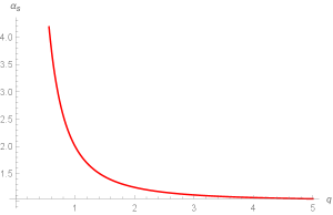
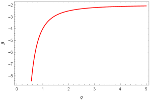
The graphs show an unphysical behavior at , this is due to the presence of dynamically generated gluon mass. The self-interacting gluons and the strong force that exist between them are capable of creating bound states with hadron degrees of freedom. These graphs depict the behavior of and observed from pQCD.
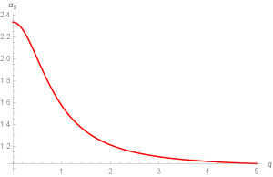
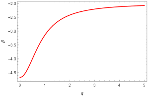
Here, the Landau singularity has been fixed by introducing the gluon mass . The presence of the gluon mass is more pronounced at and gradually vanishes in the limit . Consequently, and from the graphs.
VII Conclusion
We modified the DBI action to develop models that are capable of mimicking the phenomenon of QCD theory using an Abelian gauge field. The models were based on the behavior of opened string with its endpoints on the D-brane. In studying color particles, the endpoints of the string serve as the source and sink of the color charges. Additionally, the models are efficient in investigating glueballs when the tachyons condense and transform into glueballs with real square masses that keep them confined. Without fermions, the models are suitable for studying the bound states of gluons and the dynamics of glueballs. To study the dynamics of quarks, we showed how the model can be coupled with standard model fermions systematically. Here, the particles involved are glueball-fermion-mix in a confined state. Moreover, we demonstrated that the color dielectric function coupled with the Abelian gauge capable of causing color confinement vanishes automatically when we introduced the non-Abelian gauge field in Sec. V.2. Consequently, the presence of coupled with the Abelian gauge field was to induce non-Abelian characteristics.
We also developed one of the models to demonstrate its ability to explain some basic characteristics of strong interactions. We derived the linear and Cornell-like potentials that are used to describe color particles in phenomenological QCD. The linear potential is motivated by the string model of hadrons whilst the Cornell potential is motivated by Lattice QCD calculations. The Cornell potential is particularly important in QCD because it shows both the asymptotic freedom and color-confining behavior exhibited by the model. We also calculated the strong running coupling and the QCD -function and compared their behavior with the traditional QCD theory. However, in the model framework, we are able to fix the non-physical Landau ghost pole that occurs at the low energy region of the model by assuming the existence of gluon mass at low momentum region, . The model leads to the determination of gluon condensate and how the glueball fields contribute to the condensate.
Furthermore, the models can be discretized using path integral formalism and investigated under lattice field theory with the availability of the required computational artifacts. As observed in the model developed in Sec. VI, the linear and the Cornell-like potentials can be used to study hadron and quarkonia spectra. Other hadron properties can also be studied from these models when the appropriate spin contributions to the potential are added. Extending the models to study the characteristics of particles at a finite temperature will pave way for understanding, chiral symmetry breaking and restoration, confinement/deconfinement, and quark-gluon-plasma phase transitions. Finally, the models can be applied in investigating physical systems such as pions.
Acknowledgements.
This work was supported by Conselho Nacional de Desenvolvimento Científico e Tecnológico (CNPq) project No.: 168546/2021-3, Brazil. F.A.B. would like to thank CNPq, CAPES and CNPq/PRONEX/FAPESQ-PB (Grant No. 165/2018), for partial financial support. F.A.B. also acknowledges support from CNPq (Grant No. 312104/2018-9), Brazil.References
- (1) J. H. Schwarz, The Early Years of String Theory: A Personal Perspective, arXiv:0708.1917 [hep-th].
- (2) J. H. Schwarz, Superstring theory, Phys. Rep. 89, 223 322 (1982).
- (3) M. B. Green, J. H. Schwarz and E. Witten, Superstring Theory. Vol. I & II, Cambridge University Press, Cambridge 1987.
- (4) J. Polchinski, An Introduction to the Bosonic String, Cambridge University Press, Cambridge 2011.
- (5) C. V. Johnson, D-Brane Primer,arXiv:hep-th/0007170.
- (6) B. Zwiebach, A First Course in String Theory, Cambridge University Press, Cambridge 2004.
- (7) K. Becker, Melanie Becker and J. H. Schwarz, String Theory and M-Theory: A Modern Introduction, Cambridge University Press, Cambridge 2006.
- (8) D. J. Gross and F. Wilczek, Ultraviolet behavior of non-abelian gauge theories, Phys. Rev. Lett. 30, 1343 1346 (1973).
- (9) H. D. Politzer, Reliable perturbative results for strong interactions? Phys. Rev. Lett. 30, 1346 1349 (1973).
- (10) C. Quigg, Gauge Theories of the Strong, Weak, and Electromagnetic Interactions, Princeton University Press, USA, 2013.
- (11) L. O’Raifeartaigh, The dawning of gauge theory, Princeton Univ. Press, Princeton, NJ, USA, 1997.
- (12) P. D. B. Collins, A. D. Martin and E. J. Squires, particle Physics and Cosmology, A John Wiley & Sons, Inc., (1989) Canada.
- (13) O. Aharony, S. S. Gubser, J. Maldacena, H. Ooguri and Y. Oz, Large N Field Theories, String Theory and Gravity, Phys. Rept. 323, 183 386 (2000) arXiv:hep-th/9905111.
- (14) J. M. Maldacena, The Large N Limit of Superconformal Field Theories and Supergravity, Adv. Theor. Math. Phys. 2, 231 252 (1998) arXiv:hep-th/9711200.
- (15) M. Graña and H. Triendl, String Theory Compactifications, SpringerBriefs in Physics (2017); M. Graña, Flux compactifications in string theory: a comprehensive review, Phys. Rept. 423 91 158 (2006) arXiv:hep-th/0509003.
- (16) J. Polchinski, Introduction to Gauge/Gravity Duality, arXiv:1010.6134 [hep-th].
- (17) S. De Haro, D. R. Mayerson and J. N. Butterfield, Conceptual Aspects of Gauge/Gravity Duality, Foundations of Physics, 46, 1381 1425 (2016) arXiv:1509.09231 [physics.hist-ph].
- (18) C. Amsler, The Quark Structure of Hadrons, Springer Nature Switzerland AG, 2018.
- (19) A. Sen, Descent Relations Among Bosonic D-branes, Int. J. Mod. Phys. A 14, 4061 4078 (1999) arXiv:hep-th/9902105.
- (20) F. Bigazzi and A. L. Cotrone, String theory meets QCD, Frascati Phys. Ser. 54, 378 385 (2012).
- (21) K. Bardakci, Dual models and spontaneous symmetry breaking, Nucl. Phys. B 68, 331 348 (1974); K. Bardakci and M. B. Halpern, Explicit Spontaneous Breakdown in a Dual Model, Phys. Rev. D 10, 4230 (1974); K. Bardakci and M.B. Halpern, Explicit Spontaneous Breakdown in a Dual Model. 2. N Point Functions, Nucl. Phys. B 96, 285 306 (1975); K. Bardakci, Spontaneous Symmetry Breakdown in the Standard Dual String Model, Nucl. Phys. B 133, 297 314 (1978).
- (22) A. Sen, Stable Non-BPS Bound States of BPS D-branes, JHEP 9808, 010 (1998) arXiv:hep-th/9805019.
- (23) A. Sen, BPS D-branes on Non-supersymmetric Cycles, JHEP 9812 021 (1998); Tachyon Condensation on the Brane Antibrane System, JHEP 9808, 012 (1998) arXiv:hep-th/9805170; Type I D-particle and its Interactions, JHEP 9810, 021 (1998).
- (24) A. Sen, Spinors of Type I and Other Solitons on Brane-Antibrane Pair, JHEP 9809 023(1998).
- (25) A. Recknagel and V. Schomerus, Boundary Deformation Theory and Moduli Spaces of D-Branes, Nucl. Phys. B 545, 233 282 (1999) arXiv:hep-th/9811237; C. G. Callan, I. R. Klebanov, A. W. W. Ludwig and J. M. Maldacena, Exact Solution of a Boundary Conformal Field Theory, Nucl. Phys. B 422, 417 448 (1994) arXiv:hep-th/9402113; J. Polchinski and L. Thorlacius, Free Fermion Representation of a Boundary Conformal Field Theory, Phys. Rev. D 50, 622 626 (1994) arXiv:hep-th/9404008.
- (26) J. A. Harvey, D. Kutasov and E. J. Martinec, On the relevance of tachyons, arXiv:hep-th/0003101; P. Fendley, H. Saleur and N.P. Warner, Exact solution of a massless scalar field with a relevant boundary interaction, Nucl. Phys. B 430, 577 596 (1994) arXiv:hep-th/9406125; J. Majumder and A. Sen, Vortex Pair Creation on Brane-Antibrane Pair via Marginal Deformation, JHEP 0006, 010 (2000) arXiv:hep-th/0003124.
- (27) A. Sen, Universality of the Tachyon Potential, JHEP 9912, 027 (1999), arXiv:hep-th/9911116.
- (28) A. Sen and B. Zwiebach, Tachyon condensation in string field theory, JHEP 0003, 002 (2000) arXiv:hep-th/9912249.
- (29) A. Kostelecky and R. Potting, Expectation Values, Lorentz Invariance, and CPT in the Open Bosonic String, Phys. Lett. B 381, 89 96 (1996) arXiv:hep-th/9605088; N. Berkovits, The Tachyon Potential in Open Neveu-Schwarz String Field Theory, JHEP 0004, 022 (2000) arXiv:hep-th/0001084; W. Taylor, D-brane effective field theory from string field theory, Nucl. Phys. B 585, 171 192 (2000) arXiv:hep-th/0001201; N. Moeller and W. Taylor, Level truncation and the tachyon in open bosonic string field theory, Nucl. Phys. B 583, 105 144 (2000) arXiv:hep-th/0002237; J. A. Harvey and P. Kraus, D-Branes as Unstable Lumps in Bosonic Open String Field Theory, JHEP 0004, 012 (2000) arXiv:hep-th/0002117; R. de Mello Koch, A. Jevicki, M. Mihailescu and R. Tatar, Lumps and P-branes in Open String Field Theory; Phys. Lett. B 482, 249 254 (2000) arXiv:hep-th/0003031; N. Moeller, A. Sen and B. Zwiebach, D-branes as Tachyon Lumps in String Field Theory; JHEP 0008, 039 (2000) arXiv:hep-th/0005036.
- (30) V. A. Kostelecky and S. Samuel, The Static Tachyon Potential in the Open Bosonic String Theory, Phys. Lett. B 207, 169 173 (1988).
- (31) N. Berkovits, A. Sen and B. Zwiebach, Tachyon condensation in superstring field theory, Nuc. Phys. B 587, 147 178 (2000).
- (32) J. A. Harvey, Per Kraus, F. Larsen and E. J. Martinec, D-branes and Strings as Non-commutative Solitons, JHEP 0007, 042 (2000) arXiv:hep-th/0005031.
- (33) R. Gopakumar, S. Minwalla and A. Strominger, Noncommutative Solitons, JHEP 0005, 020 (2000) arXiv:hep-th/0003160; K. Dasgupta, S. Mukhi and G. Rajesh, Noncommutative Tachyons, JHEP 0006, 022 (2000) arXiv:hep-th/0005006; J. A. Harvey, P. Kraus and F. Larsen, Exact Noncommutative Solitons, JHEP 0012, 024 (2000) arXiv:hep-th/0010060.
- (34) A. A. Gerasimov and S. L. Shatashvili, On Exact Tachyon Potential in Open String Field Theory, JHEP 0010, 034 (2000) arXiv:hep-th/0009103; D. Kutasov, M. Marino and G. Moore, Some Exact Results on Tachyon Condensation in String Field Theory, JHEP 0010, 045 (2000) arXiv:hep-th/0009148; D. Ghoshal and A. Sen, Normalization of the Background Independent Open String Field Theory Action, JHEP 0011, 021 (2000) arXiv:hep-th/0009191; J. A. Minahan and B. Zwiebach, Field theory models for tachyon and gauge field string dynamics, JHEP 0009, 029 (2000) arXiv:hep-th/0008231; Effective Tachyon Dynamics in Superstring Theory, JHEP 0103, 038 (2001) arXiv:hep-th/0009246.
- (35) A. Sen, Fundamental Strings in Open String Theory at the Tachyonic Vacuum, J. Math. Phys. 42, 2844 2853 (2001) arXiv:hep-th/0010240.
- (36) E. Witten, Bound States Of Strings And p-Branes, Nucl. Phys. B 460,335 350 (1996) arXiv:hep-th/9510135.
- (37) U. Lindström and R. von Unge, A Picture of D-branes at Strong Coupling, Phys. Lett. B 403, 233 238 (1997) arXiv:hep-th/9704051; U. Lindström, M. Zabzine and A. Zheltukhin, Limits of the D-brane action, JHEP 9912, 016 (1999) arXiv:hep-th/9910159; U. Lindström and M. Zabzine, Strings at the Tachyonic Vacuum, JHEP 0103, 014 (2001) arXiv:hep-th/0101213.
- (38) H. Gustafsson and U. Lindstrom, A Picture of D-branes at Strong Coupling II. Spinning Partons, Phys. Lett. B 440 43 49 (1998) arXiv:hep-th/9807064.
- (39) A. Sen, Tachyon Dynamics in Open String Theory, Int. J. Mod. Phys. A 20,5513 5656 (2005) arXiv:hep-th/0410103; Tachyons in String Theory, Ann. Henri Poincaré 4, Suppl. 1, S31 S42 (2003).
- (40) E. Witten, Non-commutative geometry and string field theory, Nuc. Phys. B 268, 253 294 (1986); N. Seiberg and E. Witten, String Theory and Noncommutative Geometry, JHEP 9909, 032, (1999) arXiv:hep-th/9908142.
- (41) O. M. P. Bilaniuk, V. K. Deshpande, and E. C. G. Sudarshan, “Meta” Relativity, Am. J. Phys. 30, 718 (1962); O. M. P. Bilaniuk and E.C.G. Sudarshan, Particles beyond the light barrier, Phys. Today 22N5, 43 51 (1969).
- (42) C. M. Hull and P. K. Townsend, Unity of Superstring Dualities, Nucl. Phys. B 438, 109 137 (1995) arXiv:hep-th/9410167.
- (43) E. Witten, String Theory Dynamics In Various Dimensions, Nucl. Phys. B 443, 85 126 (1995) arXiv:hep-th/9503124.
- (44) D. J. Gross, A. Neveu, J. Scherk, and J. H. Schwarz, Renormalization and Unitarity in the Dual-Resonance Model, Phys. Rev. D 2, 697 (1970).
- (45) C. Lovelace, Pomeron form-factors and dual Regge cuts, Phys. Lett. B 34, 500 506 (1971).
- (46) B. Zwiebach, Oriented Open-Closed String Theory Revisited, Ann. Phys. 267 193 248 (1998), arXiv:hep-th/9705241.
- (47) J. Hughes, J. Liu and J. Polchinski, Supermembranes, Phys. Lett. B 180, 370 (1986).
- (48) M. Born and L. Infeld, Foundations of the new field theory, Proc. Roy. Soc. Lond. A A 144, 425 451 (1934).
- (49) G. W. Gibbons, Born-Infeld particles and Dirichlet p-branes, Nucl. Phys. B 514, 603 639 (1998) arXiv:hep-th/9709027.
- (50) P. A. M. Dirac, An Extensible model of the electron, Proc. Roy. Soc. Lond. A 268, 57 67 (1962).
- (51) J. Polchinski, S. Chaudhuri and C. V. Johnson, Notes on D-Branes, arXiv:hep-th/9602052; J. Polchinski, TASI Lectures on D-Branes, arXiv:hep-th/9611050.
- (52) W. Taylor, Lectures on D-branes, Gauge Theory and M(atrices), arXiv:hep-th/9801182.
- (53) R. G. Leigh, Dirac-Born-Infeld Action from Dirichlet Sigma Model, Mod. Phys. Lett. A 4, 2767 (1989).
- (54) E. Bergshoeff, E. Sezgin, P.K. Townsend, Supermembranes and Eleven-Dimensional Supergravity, Phys. Lett. B 189, 75 78 (1987).
- (55) P. K. Townsend, The eleven-dimensional supermembrane revisited, Phys. Lett. B 350, 184 187 (1995) arXiv:hep-th/9501068.
- (56) M. R. Garousi, Tachyon couplings on non-BPS D-branes and Dirac-Born-Infeld action, Nucl. Phys. B 584, 284 299 (2000) arXiv:hep-th/0003122.
- (57) J. Kluson, Proposal for non-BPS D-brane action, Phys. Rev. D 62 126003 (2000) arXiv:hep-th/0004106.
- (58) A. A. Tseytlin, Born-Infeld action, supersymmetry and string theory, hep-th/9908105 [hep-th].
- (59) W. Taylor, Lectures on D-branes, tachyon condensation, and string field theory, arXiv:hep-th/0301094.
- (60) W. Taylor and B. Zwiebach, D-Branes, Tachyons, and String Field Theory, arXiv:hep-th/0311017.
- (61) A. Sen, Non-BPS States and Branes in String Theory, arXiv:hep-th/9904207.
- (62) C. G. Callan, C. Lovelace, C. R. Nappi, and S. A. Yost, Loop corrections to superstring equations of motion, Nucl. Phys. B 308, 221 284 (1988). A. Abouelsaood, C. G. Callan, C. R. Nappi and S. A. Yost, Open strings in background gauge fields, Nucl. Phys. B 280, 599 624 (1987).
- (63) M. R. Garousi, Slowly varying tachyon and tachyon potential, JHEP 0305 05 (2003) arXiv:hep-th/0304145.
- (64) T. Banks, W. Fischler, S. H. Shenker and L. Susskind, M Theory As A Matrix Model: A Conjecture, Phys. Rev. D 55, 5112 5128 (1997) arXiv:hep-th/9610043.
- (65) D. Lust, Intersecting Brane Worlds — A Path to the Standard Model?, Class. Quant. Grav. 21, S1399 1424 (2004) arXiv:hep-th/0401156; I. Antoniadis, E. Kiritsis, J. Rizos and T. N. Tomaras, D-branes and the Standard Model, Nucl. Phys. B 660, 81 115 (2003) arXiv:hep-th/0210263; L. E. Ibanez, F. Marchesano and R. Rabadan, Getting just the Standard Model at Intersecting Branes, JHEP 0111, 002 (2001) arXiv:hep-th/0105155; A. Chatzistavrakidis, H. Steinacker and G. Zoupanos, Intersecting branes and a standard model realization in matrix models, arXiv:1107.0265 [hep-th].
- (66) G. ’t Hooft, A Planar Diagram Theory for Strong Interactions, Nucl. Phys. B 72, 461 (1974).
- (67) E. Witten, Baryons in the Expansion, Nucl. Phys. B 160, 57 115 (1979).
- (68) D. Mateos, String Theory and Quantum Chromodynamics, Class. Quant. Grav. 24, S713 S740 (2007) arXiv:0709.1523 [hep-th].
- (69) J. Dai, R. G. Leigh and J. Polchinski, New Connections Between String Theories, Mod. Phys. Lett. A 4, 2073 2083 (1989).
- (70) J. Polchinski, Dirichlet-Branes and Ramond-Ramond Charges, Phys. Rev. Lett. 75, 4724 4727 (1995) arXiv:hep-th/9510017.
- (71) C. G. Callan Jr. and J. M. Maldacena, Brane Dynamics From the Born-Infeld Action, Nucl. Phys. B 513, 198 212 (1998) arXiv:hep-th/9708147.
- (72) S. -J. Rey, J.-T. Yee, Macroscopic strings as heavy quarks: Large-N gauge theory and anti-de Sitter supergravity, Eur. Phys. J. C 22, 379 394 (2001) arXiv:hep-th/9803001.
- (73) S. Lee, A. Peet and L. Thorlacius, Brane-Waves and Strings, Nucl. Phys. B 514, 161 176 (1998) arXiv:hep-th/9710097.
- (74) E. Guendelman, A. Kaganovich, E. Nissimov and S. Pacheva, Space-Time Compactification/Decompactification Transitions Via Lightlike Branes, Gen. Rel. Grav. 43, 1487 1513 (2011) arXiv:1007.4893 [hep-th].
- (75) M. Gell-Mann and B. Zwiebach, Spacetime compactification induced by scalars. Phys. Lett. B 141, 333 (1984).
- (76) L. Randall and R. Sundrum, An Alternative to Compactification, Phys. Rev. Lett. 83, 4690 4693 (1999) arXiv:hep-th/9906064.
- (77) K. Shiraishi, Compactification of spacetime in Yang-Mills theory, Classical and Quantum Gravity 6, 2029 2034 (1989) arXiv:1301.6213 [hep-th].
- (78) F. A. Brito, M.L.F. Freire, W. Serafim, Confinement and screening in tachyonic matter, Eur.Phys.J. C 74, 12 3202 (2014).
- (79) A. Issifu and F. A. Brito, The (De)confinement Transition in Tachyonic Matter at Finite Temperature, Adv. Hig. Ener. Phys. 2019, 9450367 (2019).
- (80) Adamu Issifu, Julio C.M. Rocha, Francisco A. Brito, Confinement of Fermions in Tachyon Matter at Finite Temperature, Adv. High. Ener. Phys. 2021, 6645678 (2021), arXiv:2012.15102 [hep-ph].
- (81) A. Issifu and F. A. Brito, Confinement of Fermions in Tachyon Matter, Adv. High. Ener. Phys. 2020, 1852841 (2020).
- (82) A. Issifu and F. A. Brito, An Effective Model for Glueballs and Dual Superconductivity at Finite Temperature, Adv. High. Ener. Phys. 2021, 5658568 (2021), arXiv:2105.01013 [hep-ph].
- (83) M. Rosina, A. Schuh and H. J. Pirner, Lattice QCD and the soliton bag model, Nucl. Phys. A 448, 557 566 (1986).
- (84) D. Kharzeev, E. Levin, and K. Tuchin, Classical gluodynamics in curved space–time and the soft pomeron, Phys. lett. B 547, 21 30 (2002).
- (85) R. Dick, Vector and scalar confinement in gauge theory with a dilaton, Phys. Lett. B 409, 321 324 (1997).
- (86) P. Gaete and E. Spallucci, Confinement from gluodynamics in curved space-time, Phys. Rev. D 77, 027702 (2008) arXiv:0707.2738 [hep-th].
- (87) O. Bergman and M. R. Gaberdiel, Stable non-BPS D-particles, Phys. Lett. B 441 133 140 (1998); Non-BPS States in Heterotic - Type IIA Duality, JHEP 9903 013(1999).
- (88) A. Sen, Field Theory of Tachyon Matter, Mod. Phys. Lett. A 171797 1804 (2002), arXiv:hep-th/0204143.
- (89) D. Erkal, D. Kutasov, and O. Lunin, Brane-Antibrane Dynamics From the Tachyon DBI Action, arXiv:0901.4368 [hep-th].
- (90) A. Sen, Dirac-Born-Infeld Action on the Tachyon Kink and Vortex, Phys. Rev. D 68, 066008 (2003), arXiv:hep-th/0303057.
- (91) H. Bech Nielsen and S. Chadha, On How to Count Goldstone Bosons, Nucl. Phys. B 105, 445 453 (1976).
- (92) G. ’t Hooft, Topology of the Gauge Condition and New Confinement Phases in Nonabelian Gauge Theories, Nucl. Phys. B 190, 455 478 (1981).
- (93) Z. F. Ezawa and A. Iwazaki, Abelian dominance and quark confinement in Yang-Mills theories, Phys. Rev. D 25, 2681 (1982).
- (94) H. Shiba and T. Suzuki, Monopoles and string tension in QCD, Phys. Lett. B 333, 461 466 (1994) arXiv:hep-lat/9404015.
- (95) T. Suzuki and I. Yotsuyanagi, Possible evidence for Abelian dominance in quark confinement, Phys. Rev. D 42, 4257 (1990); J. D. Stack, W. W. Tucker and R. J. Wensley, Confinement in : Simple and generalized maximal Abelian gauge, arXiv:hep-lat/0205006; V. G. Bornyakov, H. Ichie, Y. Mori, D. Pleiter, M. I. Polikarpov, G. Schierholz, T. Streuer, H. Stüben, and T. Suzuki (DIK collaboration), Phys. Rev. D 70, 054506 (2004); V. G. Bornyakov, E. -M. Ilgenfritz and M. Muller-Preussker, Universality check of Abelian monopoles, Phys. Rev. D 72, 054511 (2005) hep-lat/0507021 [hep-lat]; G. S. Bali, V. Bornyakov, M. Müller-Preussker, and K. Schilling, Dual superconductor scenario of confinement: A systematic study of Gribov copy effects, Phys. Rev. D 54, 2863 (1996).
- (96) N. Sakumichi and H. Suganuma, Perfect Abelian dominance of quark confinement in QCD, Phys. Rev. D 90, 111501 (2014); Three-quark potential and Abelian dominance of confinement in QCD, Phys. Rev. D 92, 034511 (2015).
- (97) M. Neubert, Les Houches Lectures on Renormalization Theory and Effective Field Theories, arXiv:1901.06573 [hep-ph].
- (98) C. G. Bollini and J. J. Giambiagi, Dimensional Renormalization: The Number of Dimensions as a Regularizing Parameter, Nuovo Cim. B 12, 20 26 (1972)
- (99) Gerard ’t Hooft and M.J.G. Veltman, Regularization and Renormalization of Gauge Fields, Nucl. Phys. B 44 189 213 (1972).
- (100) C. Itzykson and J.B. Zuber, Quantum Field Theory, McGraw-Hill, New York, USA, 1980.
- (101) P. Pascual and R. Tarrach, QCD: Renormalization for the Practitioners, Lect. Notes Phys. 194 1 27 (1984).
- (102) M. E. Peskin and D. V. Schroeder, An Introduction to quantum field theory, Addison-Wesley (1995).
- (103) J. Collins, Foundations of perturbative QCD, Camb. Monogr. Part. Phys. Nucl. Phys. Cosmol. 32 1 624 (2011).
- (104) S. Weinberg, The Quantum theory of fields. Vol. 1: Foundations, Cambridge University Press, 2005.
- (105) S. Weinberg, The quantum theory of fields. Vol. 2: Modern applications, Cambridge University Press, 2013.
- (106) M. D. Schwartz, Quantum Field Theory and the Standard Model, Cambridge University Press, 2014.
- (107) C. N. Yang and R. L. Mills, Conservation of Isotopic Spin and Isotopic Gauge Invariance, Phys. Rev. 96, 191 (1954).
- (108) G. S. Bali, QCD forces and heavy quark bound states, Phys. Rept. 343, 1 136 (2001) arXiv:hep-ph/0001312.
- (109) M. Tanabashi et al., (Particle Data Group), Phys. Rev. D 98, 030001 (2018) and 2019 updated.
- (110) M. Albanese et al. [APE Collaboration], Glueball Masses and String Tension in Lattice QCD, Phys. Lett. B 192, 163 169 (1987).
- (111) P. Bacilieri et al. [APE Collaboration], Scaling in Lattice (QCD): Glueball Masses and String Tension, Phys. Lett. B 205, 535-539 (1988).
- (112) M. Teper, Glueballs, strings and topology in SU(N) gauge theory, Nucl. Phys. Proc. Suppl. 109 A, 134 140 (2002) arXiv:hep-lat/0112019.
- (113) C. J. Morningstar and M. Peardon, Glueball spectrum from an anisotropic lattice study, Phys. Rev. D 60, 034509 (1999).
- (114) M. Loan, X.-Q. Luo, Z.-H. Luo,Monte Carlo study of glueball masses in the Hamiltonian limit of lattice gauge theory, Int. J. Mod. Phys. A 21, 2905 2936 (2006).
- (115) Y. Chen, et al.,Glueball spectrum and matrix elements on anisotropic lattices, Phys. Rev. D 73, 014516 (2006).
- (116) W. Lee and D. Weingarten, Scalar Quarkonium Masses and Mixing with the Lightest Scalar Glueball, Phys. Rev. D 61, 014015 (2000) arXiv:hep-lat/9910008.
- (117) G. S. Bali et al., (UKQCD), A comprehensive lattice study of glueballs, Phys. Lett. B 309, 378 384 (1993) arXiv:hep-lat/9304012.
- (118) W. Heisenberg, Über den Bau der Atomkerne. I. Zeitschr. f. Phys. 77, 1 (1932); English translation in D. M. Brink, Nuclear Forces, Pergamon, Oxford, 1965, pp. 144 154.
- (119) D. Atkinson and P. W. Johnson, Current and constituent quark masses: Beyond chiral-symmetry breaking, Phys. Rev. D 41, 1661 1666 (1990).
- (120) E. Eichten, K. Gottfried, T. Kinoshita, K. D. Lane, and T. M. Yan,Charmonium: The model, Phys. Rev. D 17, 3090 3117 (1978).
- (121) G .W. Carter, O. Scavenius, I.N. Mishustin and P.J. Ellis, Phys. Rev. C 61, 045206 (2000).
- (122) A. Deur, S. J. Brodsky, G. F. de Teramond, The QCD Running Coupling, Prog. Part. Nuc. Phys. 90 1 (2016) arXiv:1604.08082 [hep-ph].
- (123) K. A. Olive et al., [Particle Data Group Collaboration], Chin. Phys. C 38, 090001 (2014); G. M. Prosperi, M. Raciti and C. Simolo, Prog. Part. Nucl. Phys. 58,387 438 (2007); G. Altarelli, PoS Corfu2012 002, (2013) 1303.6065 [hep-ph].
- (124) A. M. Badalian, A. I. Veselov and B. L. G. Bakker, Phys. Atom. Nucl. 67, 1367 1377 (2004) hep-ph/0311010 [hep-ph]; Phys. Rev. D 70, 016007 (2004); A. M. Badalian and V. L. Morgunov, Phys. Rev. D 60, 116008 (1999); A .M. Badalian and D. S. Kuzmenko, Phys. Atom. Nucl. 67, 561 563 (2004).
- (125) Yu. A. Simonov, Phys. Atom. Nucl. 74, 1223 (2011) 1011.5386 [hep-ph].
- (126) A. M. Badalian and D. S. Kuzmenko, Phys. Rev. D 65, 016004 (2001); A. M. Badalian, Phys. Atom. Nucl. 63, 2173 2183 (2000).
- (127) J. M. Cornwall, Phys. Rev. D 26, 1453 (1982).