Phenomenological model for the third-harmonic magnetic response of superconductors: application to Sr₂RuO₄

Fluctuations of a superconductor in the presence of an external magnetic field can be modeled within the phenomenological Ginzburg-Landau framework. In a regime close to $T_{c}$, the general superconducting Ginzburg-Landau free-energy functional takes the form:

Here, $\Psi\left(\mathbf{x}\right)$ is the superconducting order parameter, $m^{*}=2m$ and $e^{*}=2e$ are the mass and charge of a Cooper pair, $\mathbf{A}$ is the vector potential, and $b>0$ is a Ginzburg-Landau parameter. The coefficient $a$ is parametrized as $a=\alpha\left(T-T_{c}\right)=\alpha T_{c}\epsilon$, where $\epsilon=\frac{T-T_{c}}{T_{c}}$ is the reduced temperature and $\alpha$ a positive constant. Near $T_{c}$, but above the temperature range where critical fluctuations become important, as set by the Ginzburg-Levanyuk parameter, one assumes that the order parameter is small and slowly-varying. As a result, the quartic term in Eq. (1) can be neglected, and only Gaussian fluctuations are considered:

To obtain the Lawrence-Doniach (LD) free-energy expression, one assumes a layered superconductor and considers a magnetic field $H$ applied perpendicular to the layers. A detailed derivation can be found in standard textbooks and review papers, see for instance Refs. (Larkin and Varlamov, 2005; Mishonov and Penev, 2000). For completeness, we only highlight the main steps of the derivation and quote the results from Ref. (Larkin and Varlamov, 2005). Because of the layered nature of the system, there is a difference between in-plane and out-of-plane kinetic terms. While the former assumes the same form as in Eq. (1), the latter is described by $\delta_{z}\left|\Psi_{l+1}-\Psi_{l}\right|^{2}$, where $\delta_{z}$ is the inter-layer coupling constant and the subscript $l$ is a layer index. It is also convenient to introduce two dimensionless quantities, $h$ and $r$. By using the result $H_{c2}\left(0\right)=\frac{2m\alpha T_{c}}{e}$ for the zero-temperature critical field, we define the dimensionless applied field $h\equiv\frac{H}{H_{c2}(0)}$. Moreover, we define the dimensionless anisotropy parameter $r\equiv\frac{2\delta_{z}}{\alpha T_{c}}$, which can also be expressed in terms of the ratio between the correlation length along the $z$ direction, $\xi_{z}(0)$, and the inter-layer separation $s$, $r=\frac{4\xi_{z}^{2}\left(0\right)}{s^{2}}$. Writing the order parameter in a product form between in-plane Landau-level wave functions and plane waves propagating along the $z$ direction, one can evaluate the partition function $Z=\int{D\Psi D\Psi^{*}e^{-\frac{\Delta\mathcal{F}\left[\Psi\left(\mathbf{x}\right)\right]}{T}}}$ and then obtain the LD free-energy expression (up to a constant) (Larkin and Varlamov, 2005; Mishonov and Penev, 2000):

Here, $\Gamma(x)$ is the gamma function, the integration over the variable $\phi$ effectively sums over the layers, $v$ is the volume, and $M_{\infty}\equiv\frac{T_{c}}{\Phi_{0}s}\frac{\ln 2}{2}$ is the absolute value of the saturation magnetization at $T_{c}$, with $\Phi_{0}$ denoting the flux quantum. Similarly, the LD expression for the magnetization is given by (Larkin and Varlamov, 2005; Mishonov and Penev, 2000):

where $\psi(x)=\frac{d\ln\Gamma(x)}{dx}$ is the digamma function. By taking $h\gg\epsilon,r$ in Eq. (4), the right-hand side gives $-1$ at $\epsilon=0$, confirming that $M_{\infty}$ is the saturation magnetization at $T_{c}$. Note that this expression is valid for $h>0$; in the case of $h<0$, symmetry implies $F\left(-h\right)=F\left(h\right)$ and $M\left(-h\right)=-M\left(h\right)$. For future reference, we list the three dimensionless parameters that will be employed throughout this work:

While the anisotropy parameter $r$ is fixed, its impact on the magnetization depends on the temperature range probed. In a regime sufficently far from $T_{c}$, $r\ll\epsilon$, the system essentially behaves as decoupled layers ($r\rightarrow 0$) and Eq.(4) becomes (Larkin and Varlamov, 2005; Mishonov and Penev, 2000)

On the other hand, as $T_{c}$ is approached, the system will eventually cross over to the regime $r\gg\epsilon$. Then, the three-dimensional nature of the system cannot be neglected, and the magnetization becomes (Larkin and Varlamov, 2005; Mishonov and Penev, 2000; Kurkijärvi et al., 1972):

where $\zeta(\nu,x)$ is Hurwitz zeta function.

Therefore, as $T_{c}$ is approached from above, we expect a crossover of the temperature-dependent magnetization from 2D-like behavior to 3D-like behavior, with the crossover temperature corresponding to $\epsilon\sim r$. This general behavior is illustrated in Fig. 1, where $M$ given by Eq. (4) is plotted as a function of the reduced temperature $\epsilon$ together with the asymptotic expressions in Eqs. (6)-(7) for a fixed field value. As expected, the contribution of the superconducting fluctuations to the magnetization are negative.

It will be useful later to contrast the temperature dependence of the third-harmonic response $\overline{M_{3}}$ with that of the nonlinear magnetic susceptibility. To derive the latter, we consider the limit of small fields, i.e. when the dimensionless magnetic field is the smallest parameter of the problem, $h\ll\epsilon,r$. Going back to the main expression for the magnetization in Eq. (4), it is convenient to define $y=\frac{\epsilon+r\sin^{2}\phi}{2h}$. Since $h\ll\epsilon,r$, it follows that $y\gg 1$ and the integrand can be expanded as:

The integrals over $\phi$ can be analytically evaluated. Expanding the magnetization in odd powers of $h$,

we find the following expressions for the linear and nonlinear susceptibilities (see also Refs. (Tsuzuki and Koyanagi, 1969; Mishonov and Penev, 2000)):

Close enough to $T_{c}$, when $\epsilon\ll r$, we find the following power-law behaviors

One of the most common experimental probes of superconducting fluctuations is to apply a dc magnetic field and measure the magnetic response, see Eq. (9). The key issue with measuring the linear susceptibility $\chi_{1}$ is that the diamagnetic contribution due to the superconducting fluctuations is typically much smaller than the paramagnetic contributions from other normal-state degrees of freedom. For the nonlinear susceptibility $\chi_{3}$, however, one generally expects that the intrinsic normal-state contribution is negligible in most cases, which could in principle allow one to assess the contribution from the superconducting fluctuations in a more unambiguous fashion. Note that, while in principle the susceptibilities $\chi_{1}$ and $\chi_{3}$ are tensor quantities, our experimental setup is designed in such a way that both the excitation and detection coils are along the same axis. We therefore only measure in-plane diagonal components, which are equivalent for a tetragonal or cubic system. Hereafter we refer only to a scalar $\chi_{3}$.

Instead of applying a dc magnetic field, the experimental technique presented in Ref. (Pelc et al., 2019) and utilized here employs an ac field (of the form $H_{0}\cos{\omega}t$) and a system of coils to measure the oscillating sample magnetization. In order to determine the third-order response, a lock-in amplifier is used at the third harmonic of the fundamental frequency $\omega$, which is typically in the kHz range. If the fifth-order susceptibility is significantly smaller than the third-order susceptibility, the third harmonic response is a good measure of the third-order susceptibility. This condition was experimentally verified by measuring at the fifth harmonic, where the signal was found to be vanishingly small except extremely close to $T_{c}$, where it was still an order of magnitude smaller than the third harmonic. We can thus safely ignore the higher-order contributions. Most of the data presented here were published in Ref. (Pelc et al., 2019), and were obtained in two separate experimental setups. Low-temperature measurements on strontium ruthenate were performed in a ³He evaporation refrigerator with a custom-made set of coils. Samples of conventional superconductors were measured in a modified Quantum Design MPMS, where we used the built-in AC susceptibility coil to generate the excitation magnetic field, and a custom-made probe with small detection coils to maximize the filling factor. We estimate that the magnetization sensitivity of both setups is better than 1 nanoemu, an improvement of 1-2 orders of magnitude over standard SQUID-based instruments. This is made possible by lock-in detection, matching the impedance of the detection coils and lock-in amplifier inputs, and large filling factors of the detection coils (Drobac et al., 2013).

Although we expect the third-harmonic response to exhibit behavior similar to the third-order nonlinear susceptibility $\chi_{3}$, there are important differences, since the amplitude of the oscillating field, albeit small ($H_{0}\sim 1$ Oe), is nonzero. Thus, to provide a more direct comparison between the LD model and experiments, we directly compute the third-harmonic response, which we denote by $\overline{M_{3}}$. In our experimental setup, the signal corresponds to the Fourier transform of $\frac{\partial M}{\partial t}$ at $3\omega$,

where $M\left(\epsilon,h(t)\right)$ is obtained from Eq.(4) by substituting $h=h_{0}\cos{\omega}t$. Integration by parts gives $\overline{M_{3}}\left(\epsilon\right)=-3i\int_{-\pi}^{\pi}M(\epsilon,h_{0}\cos\theta)e^{3i\theta}d\theta$ with $\theta=\omega t$. Using the fact that $M\left(\epsilon,-h\right)=-M\left(\epsilon,h\right)$, we have $\int_{-\pi}^{-\pi/2}M(\epsilon,h_{0}\cos\theta)e^{i3\theta}d\theta=\int_{0}^{\pi/2}M(\epsilon,h_{0}\cos\theta)e^{i3\theta}d\theta$ and $\int_{\pi/2}^{\pi}M(\epsilon,h_{0}\cos\theta)e^{i3\theta}d\theta=\int_{-\pi/2}^{0}M(\epsilon,h_{0}\cos\theta)e^{i3\theta}d\theta$, which yields

where the field $h_{0}\cos\theta$ remains positive between the integration limits. Experimentally, both the imaginary and real parts can be measured. However, due to issues with lock-in phase determination in third-harmonic measurements (Drobac et al., 2013), we simply use the absolute value of $\overline{M_{3}}$ for comparison between the experimental and theoretical results.

In the temperature range where $h_{0}\ll\epsilon$, we can substitute the series expansion (9) in Eq. (17) and find:

Now, in the relevant regime $r\gg\epsilon$, according to Eqs. (14), we have $\chi_{3}\sim\epsilon^{-5/2}$ and $\chi_{5}\sim\epsilon^{-9/2}$. Therefore, as long as we remain in the regime $h_{0}\ll\epsilon$, the contribution from the fifth-order nonlinear susceptibility $\chi_{5}$ can be neglected. Using Eq. (11) we obtain:

Therefore, we expect that, in the temperature range $h_{0}\ll\epsilon\ll r$, the third-harmonic response $\left|\overline{M_{3}}\right|$ displays the power-law behavior $\left(T-T_{c}\right)^{-5/2}$ characteristic of the third-order nonlinear susceptibility $\chi_{3}$. To verify this behavior explicitly, in Fig. 2 we present the numerically calculated $|\overline{M_{3}}|$ for $h_{0}=10^{-3}$ and $r=1$, and compare it with the analytical approximation in Eq. (19). It is clear that the expected power-law behavior appears over a rather wide temperature range. As one approaches $T_{c}$ from above and reaches the temperature scale $\epsilon\sim h_{0}$, deviations from the power-law are observed, and $\left|\overline{M_{3}}\right|$ saturates to a constant value. This is a direct consequence of the fact that we are not computing the dc susceptibility, but the ac third-harmonic response at a fixed field amplitude $h_{0}$. Figs. 3(a)-(b) depict how the temperature window in which power-law behavior is observed is affected by changing $r$ and $h_{0}$. As expected, increasing $h_{0}$ significantly suppresses the window of power-law behavior, as the temperature scale $\epsilon\sim h_{0}$ is moved up. On the other hand, the anisotropy parameter $r$ has a rather minor impact on the temperature range in which $\epsilon^{-5/2}$ behavior is observed.

In order to validate the LD approach for the third-harmonic response, we first compare the theoretical results for $\overline{M_{3}}$ from Eq.(17) with the experimental third-harmonic data for three conventional elemental superconductors: lead (Pb), niobium (Nb), and vanadium (V). Besides an overall pre-factor, there are three fitting parameters in our formalism: the upper critical field $H_{c2}$, the critical temperature $T_{c}$, and the anisotropy ratio $r$. The field $H_{0}$ is 1.3 Oe as generated by the excitation coil, but the true value could be modified by demagnetization factors (especially very close and below $T_{c}$) by up to a factor of $\sim 2$. Hereafter, for concreteness, we will use $H_{0}=1.3$ Oe for all cases. Since these materials are rather three-dimensional, we expect the $z$-axis correlation length $\xi_{z}$ to be larger than the layer distance $s$ in the LD model, i.e. $r>4$. Thus, because the reduced temperatures probed are very small ($\epsilon_{\mathrm{max}}\sim 10^{-2}$), the precise value of $r$ does not significantly affect the temperature dependence of $|\overline{M_{3}}|$ in the experimentally relevant temperature regime (as shown above in Fig. 3(b)). Therefore, to minimize the number of fitting parameters, we set $r=10$ in all cases. This leaves only two free parameters, $H_{c2}$ and $T_{c}$.

The comparison between theoretical and experimental results is shown Figs. 4, 5, and 6 for Pb, Nb, and V, respectively. In all figures, the circle and square symbols correspond to data, whereas dashed and solid lines correspond to theoretical results. Experimental measurements of $\left|\overline{M_{3}}\right|$ become challenging below $\epsilon\sim 10^{-4}$ due to thermometry resolution issues, and the signal typically decays below the noise level around $\epsilon\sim 10^{-2}$, indicating a small temperature regime of significant superconducting fluctuations. In the case of V, a kink is observed in one sample (light green symbols), which is possibly a spurious signal due to solder superconductivity or the result of a slight macroscopic sample inhomogeneity. For this reason, we also include results from a second sample (dark green symbols). Because the overall magnitude of the experimental $\left|\overline{M_{3}}\right|$ is arbitrary and changes with modifications of the set-up, we rescaled the $\left|\overline{M_{3}}\right|$ values of the second sample (dark green symbols) by an overall constant to better match the behavior of $\left|\overline{M_{3}}\right|$ of the first sample (light green symbols) at larger $\epsilon$ values.

In order to obtain the best fit, we considered two slightly different procedures. In panels (a)-(b) of each figure (dashed lines), we fixed $T_{c}$ to be the temperature at which the third-harmonic response displays a maximum; we refer to this value as $T_{c}^{(\mathrm{exp})}$. It is important to note, however, that this value is not necessarily the exact temperature of zero resistance onset. For this reason, and given the intrinsic experimental uncertainties in the precise absolute determination of $T_{c}$, in panels (c)-(d) (solid lines) we allowed $T_{c}$ to vary from $T_{c}^{(\mathrm{exp})}$, but by no more than $0.5\%$. The fit parameters are shown in Table 1, together with the experimental values for $T_{c}^{(\mathrm{exp})}$ and $H_{c2}^{(\mathrm{exp})}$, the latter taken from Ref. (Lide, 2004). Note that, to distinguish between the two fitting procedures, we denote by $\tilde{H}_{c2}$ the value used in panels (a)-(b) of the figures. Moreover, since Pb is a type-I superconductor, $H_{c2}^{(\mathrm{exp})}$ was estimated through $\sqrt{2}\kappa H_{c}$ (Tinkham, 2004), with $\kappa=0.24$ (Smith, 1969; Farrell et al., 1969) and $H_{c}=803$ Oe (Smith, 1969; Martienssen and Warlimont, 2006).

Panels (a)-(b) of Figs. 4, 5, and 6 show that the theoretical curves obtained by fixing $T_{c}=T_{c}^{(\mathrm{exp})}$ provide a reasonable description of the third-harmonic data in the region not too close to $T_{c}$ for Pb and V (Figs. 4 and 6), and in the region close to $T_{c}$ for Nb (Fig. 5). In particular, the latter does not seem to display the characteristic $\epsilon^{-5/2}$ power-law behavior observed in the former two in the regime of intermediate $\epsilon$ values. However, because of the definition of the reduced temperature, $\epsilon=\frac{T-T_{c}}{T_{c}}$, even small changes in $T_{c}$ within typical experimental uncertainty could account for these deviations between theory and experiment. As noted above, to address this issue we performed a second fit procedure allowing $T_{c}$ to be slightly different than $T_{c}^{(\mathrm{exp})}$. As shown in panels (c)-(d) of the same figures, we find a better agreement between the theoretical and experimental results over a wider temperature range, including in the case of Nb in the intermediate $\epsilon$ range. Comparing the theoretical $T_{c}$ values in Table 1 with the $T_{c}^{(\mathrm{exp})}$ values, we note that in all cases $T_{c}$ is slightly larger than $T_{c}^{(\mathrm{exp})}$. This is the reason why in panels (c)-(d) the theoretical curves stop at $\epsilon=0$ whereas the data extend to the region $\epsilon<0$.

On the other hand, there is a more significant difference between $H_{c2}$ and the experimental value $H_{c2}^{(\mathrm{exp})}$ taken from the literature, with the former being a factor of approximately $2$ to $6$ smaller or larger than the latter. We note that the intrinsic uncertainty in the precise value of $H_{0}$ in our experiment may explain at least part of this discrepancy. Moreover, the value of $H_{c2}^{(\mathrm{exp})}$ strongly depends on material preparation details, especially for polycrystalline samples where significant internal strains can be present (Van Gurp, 1967). In principle, the critical fields are lower in more pristine materials, and it is therefore meaningful to take the lowest known experimental values (taken from Ref. (Lide, 2004)) for our comparison. Finally, while the LD model employed here to calculate $\left|\overline{M_{3}}\right|$ assumes a layered system, the bulk elemental superconductors are cubic. On top of that, the LD approach of including only Gaussian fluctuations is expected to break down below a very small $\epsilon_{\mathrm{crit}}$, whose precise value is likely different for distinct materials. Despite these drawbacks, this comparison shows that the LD model for the third-harmonic response $\left|\overline{M_{3}}\right|$ due to contributions from superconducting fluctuations provides a satisfactory description of the experimental results.

Having validated our theoretical approach to compute the third-harmonic response $\left|\overline{M_{3}}\right|$ by comparison with data for elemental superconductors, we now perform the same comparison with the lamellar perovskite-derived superconductor Sr₂RuO₄ (SRO). The main advantage of our LD calculation of $\left|\overline{M_{3}}\right|$ is that it is entirely phenomenological and independent of microscopic details. In fact, the main assumption is that the superconducting fluctuations can be described by a Gaussian approximation. Consequently, the calculation could in principle be applicable to unconventional superconductors as well.

SRO is believed to host an unconventional superconducting state that breaks time-reversal symmetry (Luke et al., 1998; Xia et al., 2006; Grinenko et al., 2021). Whereas for a long time SRO was considered a promising candidate for $p$-wave triplet superconductivity (Mackenzie and Maeno, 2003; Kallin, 2012), recent experiments have revealed problems with this interpretation (Mackenzie et al., 2017; Pustogow et al., 2019; Chronister et al., 2020). This has motivated alternative proposals involving e.g. $d$-wave and $g$-wave superconductivity (Røising et al., 2019; Ramires and Sigrist, 2019; Rømer et al., 2019; Suh et al., 2020; Kivelson et al., 2020; Willa et al., 2020). As mentioned above, the data presented here are the same as in Ref. (Pelc et al., 2019). As shown there, the third-harmonic response of other perovskite-based superconductors like strontium titanate and the cuprates display a similar unusual temperature dependence.

The data for SRO are shown by the orange symbols in Fig. 7 on linear scale (panel (a)), logarithmic scale (panel (b)), and semi-logarithmic scale (panel (c)). The theoretical results for $\left|\overline{M_{3}}\right|$ are plotted in the same panels using the experimental critical temperature value, $T_{c}=1.51\>\mathrm{K}=T_{c}^{(\mathrm{exp})}$, and two different critical field values: $H_{c2}=750\>\mathrm{G}=H_{c2}^{(\mathrm{exp})}$ (dashed lines) and $H_{c2}=7.6\>\mathrm{G}\approx 0.01H_{c2}^{(\mathrm{exp})}$ (dotted lines). Here, $T_{c}^{(\mathrm{exp})}$ corresponds to the temperature at which the third-harmonic response is maximum, and $H_{c2}^{(\mathrm{exp})}$ is the experimental value reported in the literature (Mackenzie and Maeno, 2003; Kittaka et al., 2009). The key observation is that the theoretical $\left|\overline{M_{3}}\right|$ curve with $H_{c2}=H_{c2}^{(\mathrm{exp})}$ grossly underestimates the data. It is necessary to reduce $H_{c2}$ by two orders of magnitude to obtain values that are comparable between theory and experiment. In contrast, for the elemental superconductors, the difference in the theoretical and experimental $H_{c2}$ values was at most a factor of $6$. More importantly, even by changing $H_{c2}$ by such a large amount, the temperature dependence of the data is not captured by the theoretical $\left|\overline{M_{3}}\right|$ curve, in contrast again to the case of conventional superconductors. Indeed, while the theoretical $\left|\overline{M_{3}}\right|$ curve shows a power-law for intermediate reduced temperatures, the data display an accurately exponential temperature dependence, as discussed in Ref. (Pelc et al., 2019) and shown in panel (c) of Fig. 7. We note that the experimental $H_{c2}$ value depends very strongly on the orientation of the field with respect to the crystalline $c$-axis, such that a small misalignment can lead to sizable variation (Kittaka et al., 2009). However, the discrepancy between the theoretical and experimental results cannot be explained by sample misalignment, since the critical field increases with increasing angle between the field direction and the crystalline $c$-axis, whereas our theoretical results require smaller $H_{c2}$ values.

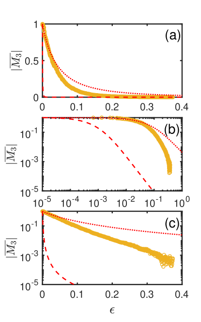
Fig. 8 summarizes the third-harmonic response $\left|\overline{M_{3}}\right|$ of the three conventional superconductors studied here (Pb, Nb, V), as well as of the unconventional superconductor SRO. The differences between SRO and the conventional superconductors are not only on the temperature dependence of $\left|\overline{M_{3}}\right|$, but also on the fact that $\left|\overline{M_{3}}\right|$ is larger and extends over a much wider relative temperature range in SRO. Indeed, while superconducting fluctuations are detected up to $\epsilon\sim 10^{-2}$ in conventional superconductors, they extend all the way up to $\epsilon\sim 1$ in SRO.

To attempt to address the discrepancy between the theoretical and experimental results for SRO, we revisit the assumptions behind the LD model, from which we derived the expression for $\left|\overline{M_{3}}\right|$. As discussed above, the LD model makes no reference to the microscopic pairing mechanism. However, it does assume a homogeneous system. In contrast, perovskites are known for their intrinsic inhomogeneity, arising from e.g. oxygen vacancies and local structural distortions that deviate strongly from the average lattice structure (see (Pelc et al., 2021) and references therein). Indeed, the experiments of Ref. (Pelc et al., 2019) indicate that universal structural inhomogeneity is present in perovskite-based superconductors such as SRO. It has also been argued that dislocations can have a strong impact on the superconducting state properties of several perovskites (Ying et al., 2013; Hameed et al., 2020; Willa et al., 2020). In the particular case of SRO, muon spin-rotation measurements find a rather inhomogeneous signature of time-reversal symmetry-breaking below $T_{c}$ (Grinenko et al., 2021). It is also known that the $T_{c}$ of SRO is strongly dependent on stress (Steppke et al., 2017; Grinenko et al., 2021), implying that inhomogeneous internal stresses would lead to regions with locally modified $T_{c}$. Simple point disorder also leads to a variation of the local critical temperature (Mackenzie et al., 1998). Indeed, scanning SQUID measurements have directly detected $T_{c}$ inhomogeneity on the micron scale (Watson et al., 2018).

The impact of inhomogeneity on superconducting properties has been studied by a variety of approaches (Coleman et al., 1995; Andersen et al., 2006; Swanson et al., 2014; Pelc et al., 2018; Dodaro and Kivelson, 2018). Here, we consider a phenomenological approach that introduces a probability distribution of the local $T_{c}$ (see also Ref. (Mayoh and García-García, 2015)). Such an inhomogeneous $T_{c}$ distribution may explain why the superconducting fluctuations in SRO are stronger and extend to higher reduced temperatures as compared to conventional superconductors, since regions with a locally higher $T_{c}$ are expected to result in a much larger contribution to $\left|\overline{M_{3}}\right|$ than that arising from the rest of the sample. To test this idea, we include a distribution function for $T_{c}$ into our LD-based phenomenological model. We denote the “transition temperature variable” as $t_{c}$, and reserve the notation $T_{c}$ for the actual transition temperature of the system to avoid confusion. The form of the distribution function $P(t_{c})$ depends on several sources of inhomogeneity in the system, see for instance Ref. (Dodaro and Kivelson, 2018). A microscopic derivation is thus very challenging, and beyond the scope of this work. Instead, here we opt for a simple phenomenological modeling of $P(t_{c})$. In particular, we employ a normalized log-normal distribution:

where $\mu$ and $\sigma$ are positive parameters that determine the mean value and variance of the distribution. The choice of this distribution is motivated by its properties of only allowing non-zero values of $t_{c}$ and of having long tails toward larger values of $t_{c}$. We note that a log-normal distribution for the local gap – and consequently of the local $T_{c}$ – was previously derived theoretically in Ref. (Mayoh and García-García, 2015) for disordered quasi-two-dimensional superconductors in the limit of weak multifractality, and observed experimentally in weakly disordered monolayer NbSe₂ (Rubio-Verdú et al., 2020). The averaged fluctuation magnetization in Eq.(4) acquires the following form:

with $M\left(\epsilon\right)$ given by Eq. (4). We can then compute the averaged third-harmonic response $\left\langle\left|\overline{M_{3}}\right|\right\rangle$ from Eq. (17). We assume that $\left\langle\left|\overline{M_{3}}\right|\right\rangle$ is dominated by superconducting fluctuations contributions, which appear only in regions that are locally non-superconducting (i.e. for which $\epsilon=\frac{T}{t_{c}}-1$ is positive). For this reason, the limits of the $t_{c}$ integration are such that $0<t_{c}<T$.

The two parameters characterizing the distribution function, $\mu$ and $\sigma$, are not independent, since they are related by the value of $T_{c}$. To see that, we first define the temperature-dependent superconducting volume fraction $v_{F}\left(T\right)$, which is given by

since the integral on the right-hand side gives the non-superconducting volume fraction ($T>t_{c}$). When the volume fraction becomes larger than a threshold value $v_{F}^{*}$, the local superconducting regions are expected to percolate and the whole sample becomes superconducting. Note that a similar criterion was used in the analysis of Ref. (Mayoh and García-García, 2015). $T_{c}$ is then obtained by solving the equation $v_{F}\left(T_{c}\right)=v_{F}^{*}$,

where $\mathrm{erf}^{-1}(x)$ is the inverse error function. For simplicity, we use for $v_{F}^{*}$ the site percolation threshold value for a cubic lattice, $v_{F}^{*}=0.3$. While $v_{F}^{*}$ itself could be considered a free parameter, we opt to fix it to avoid increasing the number of fitting parameters. As a result, the only additional parameter needed to compute $\left\langle\left|\overline{M_{3}}\right|\right\rangle$, as compared to the “clean” system $\left|\overline{M_{3}}\right|$, is the dimensionless $\sigma$, which determines the width of the distribution. In Fig. 9(a), we illustrate the profile of $P\left(t_{c}\right)$ for different values of $\sigma$ under the constraint $v_{F}\left(T_{c}^{(\mathrm{exp})}\right)=0.3$. The full expression for $\left\langle\left|\overline{M_{3}}\right|\right\rangle$ then becomes:

with:

Using the distribution functions of Fig. 9(a), in Fig. 9(b) we present the calculated averaged third-harmonic response $\left\langle\left|\overline{M_{3}}\right|\right\rangle$ (solid red line) using the experimentally determined values for $T_{c}$ and $H_{c2}$. The comparison with the data shows that even a relatively mild width of the distribution of $t_{c}$ values, with $\sigma\apprle 0.1$, is capable of capturing the extended temperature window for which the third-harmonic response is sizable. As anticipated, this behavior is a consequence of the fact that regions with a local higher $T_{c}$ value, although occupying a small volume, provide a sizable contribution to the third-harmonic response.

The temperature dependence of the third-harmonic response data, however, is not very well captured by the theoretical curves in Fig. 9(b). To try to address this issue, we promote $T_{c}$ to a free parameter and allow it to deviate slightly from the experimental value $T_{c}^{(\mathrm{exp})}=1.51$ K. Fig. 10 shows the results for $\left\langle\left|\overline{M_{3}}\right|\right\rangle$ in the case of $T_{c}=1.41\>\mathrm{K}\approx 0.93T_{c}^{(\mathrm{exp})}$ and $\sigma=0.08$. Clearly, the temperature dependence of the calculated $\left\langle\left|\overline{M_{3}}\right|\right\rangle$ becomes more similar to the experimentally measured one, but still fails to capture it completely. Thus, our conclusion is that while $T_{c}$ inhomogeneity may explain the extended temperature range where the third-harmonic response is sizable, it is unlikely to explain the exponential tail of $\left|\overline{M_{3}}\right|$ observed experimentally in Ref. (Pelc et al., 2019).