Present Address: ]NTT Secure Platform Laboratories, NTT Corporation, Musashino 180-8585, Japan
Present Address: ]Integrated Research for Energy and Environment Advanced Technology, Kyushu Institute of Technology, Kitakyushu, Fukuoka 804-8550, Japan
Phenomenological analysis of transverse thermoelectric generation and cooling performance in magnetic/thermoelectric hybrid systems
Abstract
We phenomenologically calculate the performance of the recently-observed Seebeck-driven transverse thermoelectric generation (STTG) for various systems in terms of the thermopower, power factor, and figure of merit to demonstrate the usefulness of STTG. The STTG system consists of a closed circuit comprising thermoelectric and magnetic materials which exhibit the Seebeck and anomalous Hall effects, respectively. When a temperature gradient is applied to the hybrid system, the Seebeck effect in the thermoelectric material layer generates a longitudinal charge current in the closed circuit and the charge current subsequently drives the anomalous Hall effect in the magnetic material layer. The anomalous Hall voltage driven by the Seebeck effect has a similar symmetry to the transverse thermoelectric conversion based on the anomalous Nernst effect. We find that the thermoelectric properties of STTG can be much better than those of the anomalous Nernst effect by increasing the Seebeck coefficient and anomalous Hall angle of the thermoelectric and magnetic materials, respectively, as well as by optimizing their dimensions. We also formulate the electronic cooling performance in the STTG system, confirming the reciprocal relation for the hybrid transverse thermoelectric conversion.
I Introduction
Thermoelectric power generation based on transverse thermoelectric phenomena has been actively investigated in spin caloritronics.Bauer2012NatMaterReview ; Boona2014Ene&EngSciReview ; Uchida2016ProcIEEESSEReview ; Mizuguchi2019STAMreview ; Uchida2021APL In particular, the anomalous Nernst effect (ANE), in which the thermoelectric voltage appears perpendicular to the direction of a temperature gradient and magnetization in magnetic materials, has gained much interest owing to its physical mechanism and thermoelectric functionalities. ANE enables thermoelectric generation with a simple thermopile structure and a convenient scaling behavior.Sakuraba2013APExThermopile ; Sakuraba2015ScrMaterANETEG ; Yang2017AIPAdvCoiledWire By utilizing the features of ANE, a coil-shaped thermoelectric generator and a flexible heat flux sensor have recently been demonstrated.Yang2017AIPAdvCoiledWire ; ZhouAPL2020heatflux
For applications of the transverse thermoelectric generation, a large transverse thermopower of is at least necessary according to the estimation in Ref. Sakuraba2015ScrMaterANETEG, . To realize such large transverse thermopower, ANE has been investigated in various materials including ferromagnetic alloys,Mizuguchi2012APEXFePtFilm ; Hasegawa2015APLOrderedAlloyFilm ; Isogami2017APExFe4Nfilm ; Seki2018JphysDFePtfilm ; Nakayama2019PRMateFeGa ; Sakai2020NatureFe3Ga Heusler compounds,Sakai2018NatPhysCo2MnGa ; Reichlova2018APLCo2MnGafilm ; Park2020PRBCMGthikcness ; Sakuraba2020PRBCMAS ; SakurabaCMG and permanent magnets.Miura2019APLSmCo5 ; MiuraAPL2020Tempdep Multilayer films may produce large transverse thermoelectric voltage with increasing the number of layers.Uchida2015PRBMultiLayer ; Fang2016PRBPtComultilayer ; Ramos2019APLFe3O4/Pt ; Seki2021PRB However, the obtained transverse thermopower is still much smaller than ; further materials exploration and device engineering are necessary to obtain larger transverse thermopower.
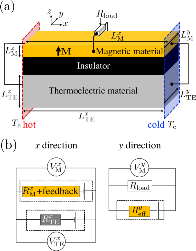
Recently, Zhou et al. proposed and experimentally demonstrated a transverse thermoelectric generation with a similar symmetry to ANE but a different driving principle from ANE. Zou2020 The device used in this experiment consists of a closed circuit comprising thermoelectric and magnetic materials which show the Seebeck effect and anomalous Hall effect (AHE), respectively. When a temperature gradient is applied to the hybrid structure in the direction, the Seebeck effect in the thermoelectric material layer generates a charge current in the closed circuit and the charge current subsequently drives AHE in the magnetic material layer [see Fig. 1(a)]. The anomalous Hall voltage driven by the Seebeck-effect-induced charge current has the same symmetry as the transverse thermoelectric conversion based on ANE when the magnetization is along the direction, boosting the transverse thermopower in the magnetic layer. Zhou et al. observed a giant transverse thermopower of 82.3 in a /n-type Si hybrid structure, which is more than 10 times larger than the anomalous Nernst coefficient of a monolayer. The observed effect is referred to as the Seebeck-driven transverse thermoelectric generation (STTG).Zou2020 They also demonstrated that the sign of the transverse thermopower induced by STTG can be changed by reversing the sign of the Seebeck coefficient of the thermoelectric material layer; a negative transverse thermopower of was observed in a /p-type Si structure.Zou2020 The previous work, however, focused only on a few combinations of thermoelectric and magnetic materials.
In this study, we phenomenologically calculate the thermopower, power factor, and figure of merit for STTG for various combinations of thermoelectric and magnetic materials to demonstrate the usefulness of STTG. The STTG system can exhibit much better performance than existing ANE materials by optimizing transport properties and dimensions of the thermoelectric and magnetic materials. Our results thus give strategies to realize efficient STTG-based energy harvesting and heat sensing devices. To confirm the reciprocal relation for the hybrid transverse thermoelectric conversion, we also formulate the electronic cooling performance in the STTG system.
II Model and setup
The following phenomenological equations for the electric field and heat current density describes the transport properties in the STTG system:Harman1962JAPTheoryNernst ; Landau ; Uchida2016ProcIEEESSEReview
| (1) | ||||
| (2) |
where , , and are the charge current density, the temperature gradient, and the unit vector along , respectively. is the longitudinal resistivity, the Seebeck coefficient, the thermal conductivity, the anomalous Hall resistivity, the anomalous Nernst coefficient, and the Righi-Leduc coefficient.Zhang2000LeducRighi1 ; Li2017LeducRighi2 Here, we neglect the thickness dependence of the transport coefficients and the magnetic field and magnetization dependences of , , and for simplicity. Note that this formalism can also be applied to the ordinary transverse transport phenomena by replacing in Eqs. (1) and (2) with a magnetic field. In our model calculation, we assume that the STTG system is in the isothermal condition in the direction, ,Harman1962JAPTheoryNernst ; Uchida2016ProcIEEESSEReview and that charge and heat currents in the direction are perfectly blocked by an ideal insulator. Thus, the following calculation is independent of the dimensions of the insulator layer depicted in Fig. 1(a). In practice, the insulator layer should be as thin as possible because a heat current in the layer does not contribute to the thermoelectric conversion. In the following calculations, for simplicity, we neglect the interface effect at the junctions of each layer, although the interface effect may affect the transport properties when the thicknesses of the thermoelectric and magnetic layers are small.Uchida2015PRBMultiLayer ; Fang2016PRBPtComultilayer ; Ramos2019APLFe3O4/Pt ; Seki2021PRB
To determine the temperature gradients in the thermoelectric and magnetic materials, we solve with the following boundary conditions: at and at . Here, is the temperature in the thermoelectric (magnetic) material, is the temperature of the hot (cold) reservoir, and is the length of the thermoelectric (magnetic) material in the direction. The notations for the dimensions along the and directions are defined in a similar manner. We set following the configuration depicted in Fig. 1(a). With the above conditions, we obtain
| (3) | ||||
| (4) |
where we assumed and . Here, , , and are the resistivity, the thermal conductivity, and the charge current density of the thermoelectric (magnetic) material, respectively, is the charge current density in the magnetic material in the direction, and .
To calculate the thermoelectric performance in the STTG system, we need to solve Eq. (1) with the boundary conditions obtained from the equivalent circuits shown in Fig. 1(b): , , and , where and are the charge currents in the thermoelectric (magnetic) material in the and directions, respectively, is the voltage in the thermoelectric (magnetic) material in the direction, is the voltage in the magnetic material in the direction, and are the electric fields, and is the load resistance. In the following calculation, we use the value of at .Harman1962JAPTheoryNernst
III Results and discussions
III.1 Transverse thermopower
By solving Eq. (1) with the aforementioned boundary conditions, we obtain the transverse thermopower for the STTG system as
| (5) |
where is the Seebeck coefficient of the thermoelectric (magnetic) material and is the size ratio between the thermoelectric and magnetic materials; see Methods in Ref. Zou2020, for further details of the derivation. Equation (5) shows that the transverse thermopower for the STTG system can be enhanced owing to the superposition of the ANE contribution in the magnetic layer (first term) and the Seebeck-driven AHE: the STTG contribution (second term). Importantly, the second term can be designed by the combination of the thermoelectric and magnetic layers as well as their dimensions, i.e., . With increasing , the second term becomes effective and approaches , where is the anomalous Hall angle of the magnetic layer. Therefore, a large second term needs large values of , , and because for typical materials.
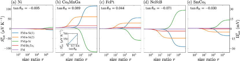
We demonstrate the behavior of using the parameters of typical thermoelectric materials (n-type Si(1), n-type Si(2), p-type Si, and ) and magnetic materials (Ni, , -ordered FePt, NdFeB, and ) shown in Table 1, where n-type Si(1) and (2) have different transport properties and hereafter "type" is omitted. is a Heusler ferromagnet showing large AHE and ANE.Sakai2018NatPhysCo2MnGa ; Reichlova2018APLCo2MnGafilm ; SakurabaCMG , -ordered FePt is often used in spintronics because it has a strong perpendicular magnetic anisotropy in a thin film form. Seki2008NmatFePt1 ; Seki2011APLFePt2 NdFeB and are rare-earth permanent magnets in practical use, which are known to exhibit substantially large AHE. Miura2019APLSmCo5 In the previous work by Zhou et al., Ni, , and FePt were used for the experimental demonstration of STTG. Zou2020 Figure 2(a) [2(b)] shows as a function of for the combination of the thermoelectric materials and Ni (). In the case of Ni with negative , the second term of Eq. (5) is negative (positive) for n(p)-Si because of negative (positive) and can be larger than owing to large when is large. We also find that the value at which the Seebeck-driven contribution is apparent with respect to for n-Si(1) and p-Si is larger than that for n-Si(2) and due to small of n-Si(2) and . As shown in Fig. 2(b), the second term of Eq. (5) for with positive has the opposite sign to that for Ni for the same thermoelectric material. Importantly, when the magnetic material with large is used, we can obtain the transverse thermopower of , which is more than an order of magnitude larger than of . The STTG contribution can further be increased in proportion to , as exemplified in the inset to Fig. 2(b). In Figs. 2(c)-2(e), we show the behavior of as a function of for -ordered FePt [Fig. 2(c)], NdFeB [Fig. 2(d)], and [Fig. 2(e)], which enable STTG in the absence of external magnetic fields owing to their large coercive force and remanent magnetization.Miura2019APLSmCo5 ; Zou2020 We find that NdFeB with relatively large exhibits a larger STTG contribution than FePt and , although of NdFeB is smaller than that of FePt and .Miura2019APLSmCo5 These demonstrations show that the transverse thermopower induced by STTG can be more than an order of magnitude larger than that induced by ANE by optimizing the combination of the thermoelectric and magnetic materials as well as their dimensions.
Here, we show that the insulator layer in Fig. 1 is important to obtain large STTG. For the system in which thermoelectric and magnetic materials are directly connected in the direction, we can derive the transverse thermopower by solving Eq. (1) with the boundary condition based on the Maxwell’s equations: . When the closed circuit is formed in the direction, the equivalent circuit in the direction gives . The transverse thermopower in this case is calculated as
| (6) |
where we assume and the linear temperature gradient along the direction for simplicity. Here, is the effective transverse resistivity of the STTG system Zou2020 :
| (7) |
Since the shunting factor , we obtain smaller transverse thermopower when the thermoelectric and magnetic materials are directly connected: . In the following, therefore, we focus only on the case shown in Fig. 1.
III.2 Power factor
We next discuss the power factor (PF) for the STTG system. To derive PF,Zou2020 we first calculate the maximum output power generated by the transverse thermoelectric voltage, , with respect to the load resistance. We calculate the maximum power as follows:
| (8) |
where we used with . We then normalize by the temperature gradient and the volume of the magnetic material and obtain PF for the STTG system as
| (9) |
This expression becomes equivalent to the power factor for ANE, , by taking the limit . Since the second term of Eq. (7) is usually small, the parameter dependence of PF is determined mainly by . Although PF in Eq. (9) can be one or two orders of magnitude larger than that for ANE with appropriate choice and design of materials in a similar manner to , the difference between the volume of the magnetic material and the total volume of the STTG system should be taken into account to discuss the thermoelectric performance and efficiency of STTG.
| Thermoelectric materialsQiao2019ACSBe2Te3 ; Zou2020 | ||||||
|---|---|---|---|---|---|---|
| n-Si(1) | ||||||
| n-Si(2) | ||||||
| p-Si | ||||||
| Magnetic materialsMiura2019APLSmCo5 ; Miura2020PRM ; Sakai2018NatPhysCo2MnGa ; Zou2020 | ||||||
| Ni | ||||||
| FePt | ||||||
| NdFeB | ||||||
III.3 Figure of merit
Now, we are in a position to discuss the figure of merit for the transverse thermoelectric conversion in the STTG system. We maximize the efficiency with respect to the load resistance , where is the heat current from the hot reservoir in the thermoelectric (magnetic) material in the direction. We then obtain the maximum efficiency as
| (10) |
where is the Carnot efficiency and is the average temperature of the hot and cold reservoirs. Here
| (11) |
is the isothermal figure of merit for the STTG system, where
| (12) |
is the effective thermal conductivity of the STTG system with being the thermal conductivity of the thermoelectric (magnetic) material. Here, , which is a characteristic of the isothermal figure of merit for the transverse thermoelectric conversion.Harman1962JAPTheoryNernst In the same manner as and PF, reduces to the isothermal figure of merit for ANE Harman1962JAPTheoryNernst when .
Although is a complicated function of parameters of thermoelectric and magnetic materials, can be enhanced for a combination of a magnetic material with large and a thermoelectric material with large figure of merit for the Seebeck effect, , as discussed in Ref. Zou2020, . This can be intuitively understood with naive approximations as follows. The second term of [Eq. (7)] and the third term of [Eq. (12)] are negligibly small for usual materials. In addition, we assume and consider only the STTG contribution in . With these approximations, we find that the figure of merit for STTG takes its maximum of at . This approximation means that a maximum value of the figure of merit for STTG is mainly determined by and .
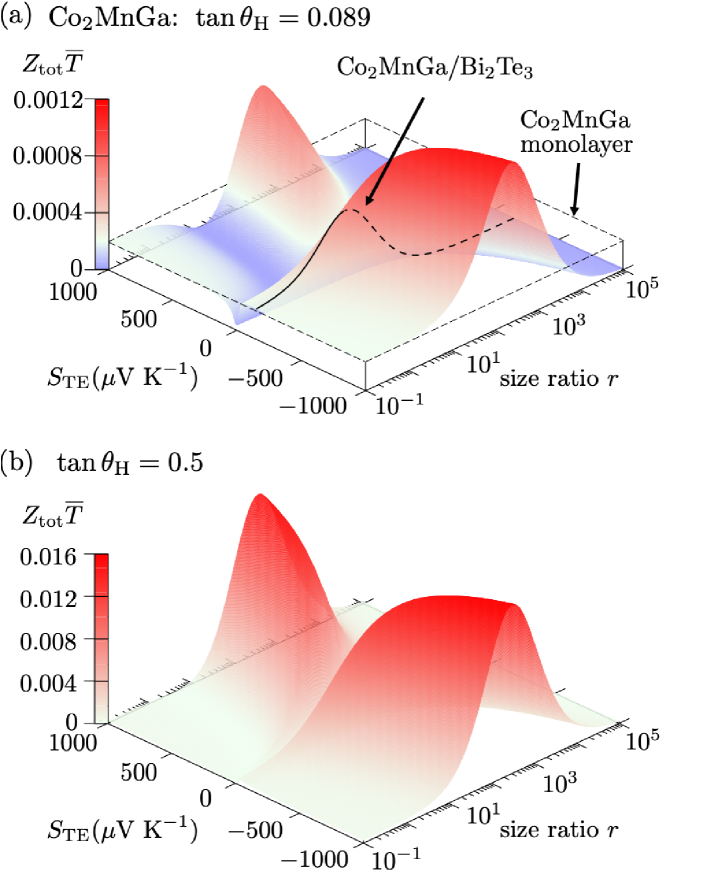
The behaviors of are exemplified in Fig. 3 (note that the aforementioned approximations are not applied here). Figure 3(a) shows for at as a function of and . Although is treated as a parameter, and are fixed at the values for , i.e., , where the black curve in Fig. 3(a) shows the case for the / junction with the parameters shown in Table 1. By choosing optimal , can be larger than the figure of merit for ANE in both for positive and negative values. The difference in the maximum between positive and negative values is attributed to the offset in Eq. (5); the situation depends on the sign and magnitude of . As shown in Fig. 3(b), when is assumed, the maximum value of is dramatically improved in comparison with the figure of merit for ANE in . Here, due to the dominant contribution of STTG, the significant improvement of appears both for positive and negative values. This demonstration shows that not only and PF but also can be enhanced by AHE driven by the Seebeck effect.
III.4 Thermoelectric cooling
Finally, we mention that the STTG system also works as a transverse thermoelectric temperature modulator by replacing the load resistance with an external battery in Fig. 1. The external battery induces a charge current in the direction, and the charge current is bent in the direction by AHE. When the charge current in the direction flows in the closed circuit comprising the thermoelectric and magnetic materials, heat is generated or absorbed at the junctions by the Peltier effect. This is the reciprocal process of STTG. The resultant temperature gradient under the adiabatic condition in the direction is calculated as follows. Since we use the same boundary conditions for , the temperature gradients in the thermoelectric and magnetic materials are the same as Eqs. (3) and (4), respectively. By solving Eq. (1) with the boundary conditions , , we obtain and as follows:
| (13) | ||||
| (14) |
where is the resistance of the thermoelectric (magnetic) material in the direction, is the anomalous Hall resistance, and is the effective resistance in the magnetic material in the direction. Using Eq. (13) and , we obtain the resultant temperature gradient under the adiabatic condition in the direction as follows:
| (15) |
where we assumed and the linear temperature gradient in the direction for simplicity. Here, is the transverse charge-to-heat conversion coefficient for the STTG system defined as
| (16) |
where is the heat current density in the thermoelectric (magnetic) material in the direction. We note that, in the definition of , the aforementioned adiabatic condition in the direction is not assumed. The coefficient satisfies the reciprocal relation (see the right longitudinal axis in Fig. 2). By taking the limit , reduces to the anomalous Ettingshausen coefficient, , and the temperature gradient in Eq. (15) reduces to that for the anomalous Ettingshausen effect.Seki2018JphysDFePtfilm ; Seki2018APL
We define the coefficient of performance (COP) for the STTG system as
| COP | ||||
| (17) |
where is the voltage of the external battery and is the effective thermal conductance of the STTG device. Here, we used Eqs. (2)-(4) and (13) for the numerator, and Eq. (14) for the denominator. To cool the STTG system, the heat current should be absorbed from the cold reservoir, , and this gives the following condition for the temperature difference:
| (18) |
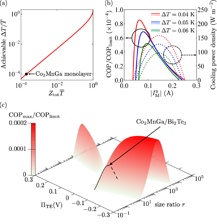
We show the upper bound of in Fig. 4(a); this is the achievable for a given . Figure 4(b) shows the dependence of COP and the cooling power density defined as . The behaviors are similar to those for the conventional Peltier and Ettingshausen effects.Mobarak2021PRAppl The maximum COP with respect to is calculated to be
| (19) |
where is the achievable limit of COP. Equation (19) reduces to the maximum COP for the anomalous Ettingshausen effectHarman1962JAPCOP when . for the STTG system can be larger than that for the anomalous Ettingshausen effect alone; its behavior is similar to that of [compare Fig. 4(c) with 3(a)].
IV Conclusion
We have phenomenologically calculated the thermoelectric properties of STTG for various combinations of thermoelectric and magnetic materials and demonstrated its usefulness. We have shown that, by combining a thermoelectric material with a large Seebeck coefficient and a magnetic material with a large anomalous Hall angle, not only the transverse thermopower but also the figure of merit for STTG can be much larger than those for conventional ANE. We have also discussed the reciprocal process of STTG; the combination of AHE in a magnetic material and the Peltier effect in a thermoelectric material enables transverse charge-to-heat conversion. It is worth mentioning that STTG works even if the thermoelectric material is also ferromagnetic, although the formulation becomes complicated. Thus, the experimental demonstration of STTG in all-ferromagnetic systems is desired. The phenomenological model for STTG will invigorate materials science research and device engineering in spin caloritronics, paving the way for versatile energy harvesting, heat sensing, and thermal management applications.
Acknowledgements.
This work was supported by CREST “Creation of Innovative Core Technologies for Nano-enabled Thermal Management” (Grant No. JPMJCR17I1) and PRESTO “Scientific Innovation for Energy Harvesting Technology” (Grant No. JPMJPR17R5) from JST, Japan, and Mitou challenge 2050 (Grant No. P14004) from NEDO, Japan. A. M. was supported by JSPS through Research Fellowship for Young Scientists (Grant No. JP18J02115).Data Availability
The data that support the findings of this study are available from the corresponding author upon reasonable request.
References
- (1) G. E. W. Bauer, E. Saitoh, and B. J. Van Wees, Nat. Mater. 11, 391 (2012).
- (2) S. R. Boona, R. C. Myers, and J. P. Heremans, Energy Environ. Sci. 7, 885 (2014).
- (3) K. Uchida, H. Adachi, T. Kikkawa, A. Kirihara, M. Ishida, S. Yorozu, S. Maekawa, and E. Saitoh, Proc. IEEE 104, 1946 (2016).
- (4) M. Mizuguchi and S. Nakatsuji, Sci. Tech. Adv. Mater. 20, 262 (2019).
- (5) K. Uchida, W. Zhou, and Y. Sakuraba, Appl. Phys. Lett. 118, 140504 (2021).
- (6) Y. Sakuraba, K. Hasegawa, M. Mizuguchi, T. Kubota, S. Mizukami, T. Miyazaki, and K. Takanashi, Appl. Phys. Express 6, 033003 (2013).
- (7) Y. Sakuraba, Scr. Mater. 111, 29 (2016).
- (8) Z. Yang, E. A. Codecido, J. Marquez, Y. Zheng, J. P. Heremans, and R. C. Myers, AIP Adv. 7, 095017 (2017).
- (9) W. Zhou and Y. Sakuraba, Appl. Phys. Express 13, 043001 (2020).
- (10) M. Mizuguchi, S. Ohata, K. Uchida, E. Saitoh, and K. Takanashi, Appl. Phys. Express 5, 093002 (2012).
- (11) K. Hasegawa, M. Mizuguchi, Y. Sakuraba, T. Kamada, T. Kojima, T. Kub- ota, S. Mizukami, T. Miyazaki, and K. Takanashi, Appl. Phys. Lett. 106, 252405 (2015).
- (12) S. Isogami, K. Takanashi, and M. Mizuguchi, Appl. Phys. Express 10, 073005 (2017).
- (13) T. Seki, R. Iguchi, K. Takanashi, and K. Uchida, J. Phys. D: Appl. Phys. 51, 254001 (2018).
- (14) H. Nakayama, K. Masuda, J. Wang, A. Miura, K. Uchida, M. Murata, and Y. Sakuraba, Phys. Rev. Mater. 3, 114412 (2019).
- (15) A. Sakai, S. Minami, T. Koretsune, T. Chen, T. Higo, Y. Wang, T. Nomoto, M. Hirayama, S. Miwa, D. Nishio-Hamane, F. Ishii, R. Arita, and S. Nakat- suji, Nature (London) 581, 53 (2020).
- (16) A. Sakai, Y. P. Mizuta, A. A. Nugroho, R. Sihombing, T. Koretsune, M.-T. Suzuki, N. Takemori, R. Ishii, D. Nishio-Hamane, R. Arita, P. Goswami, and S. Nakatsuji, Nat. Phys. 14, 1119 (2018).
- (17) H. Reichlova, R. Schlitz, S. Beckert, P. Swekis, A. Markou, Y.-C. Chen, D. Kriegner, S. Fabretti, G. Hyeon Park, A. Niemann, S. Sudheendra, A. Thomas, K. Nielsch, C. Felser, and S. T. B. Goennenwein, Appl. Phys. Lett. 113, 212405 (2018).
- (18) G.-H. Park, H. Reichlova, R. Schlitz, M. Lammel, A. Markou, P. Swekis, P. Ritzinger, D. Kriegner, J. Noky, J. Gayles, Y. Sun, C. Felser, K. Nielsch, S. T. B. Goennenwein, and A. Thomas, Phys. Rev. B 101, 060406 (2020).
- (19) Y. Sakuraba, K. Hyodo, A. Sakuma, and S. Mitani, Phys. Rev. B 101, 134407 (2020).
- (20) K. Sumida, Y. Sakuraba, K. Masuda, T. Kono, M. Kakoki, K. Goto, W. Zhou, K. Miyamoto, Y. Miura, T. Okuda, and A. Kimura, Commun. Mater. 1, 89 (2020).
- (21) A. Miura, H. Sepehri-Amin, K. Masuda, H. Tsuchiura, Y. Miura, R. Iguchi, Y. Sakuraba, J. Shiomi, K. Hono, and K. Uchida, Appl. Phys. Lett. 115, 222403 (2019).
- (22) A. Miura, K. Masuda, T. Hirai, R. Iguchi, T. Seki, Y. Miura, H. Tsuchiura, K. Takanashi, and K. Uchida, Appl. Phys. Lett. 117, 082408 (2020).
- (23) K. Uchida, T. Kikkawa, T. Seki, T. Oyake, J. Shiomi, Z. Qiu, K. Takanashi, and E. Saitoh, Phys. Rev. B 92, 094414 (2015).
- (24) C. Fang, C. H. Wan, Z. H. Yuan, L. Huang, X. Zhang, H. Wu, Q. T. Zhang, and X. F. Han, Phys. Rev. B 93, 054420 (2016).
- (25) R. Ramos, T. Kikkawa, A. Anadón, I. Lucas, T. Niizeki, K. Uchida, P. A. Algarabel, L. Morellón, M. H. Aguirre, M. R. Ibarra, and E. Saitoh, Appl. Phys. Lett. 114, 113902 (2019).
- (26) T. Seki, Y. Sakuraba, K. Masuda, A. Miura, M. Tsujikawa, K. Uchida, T. Kubota, Y. Miura, M. Shirai, and K. Takanashi, Phys. Rev. B 103, L020402 (2021).
- (27) W. Zhou, K. Yamamoto, A. Miura, R. Iguchi, Y. Miura, K. Uchida, and Y. Sakuraba, Nat. Mater. 20, 463 (2021).
- (28) T. C. Harman and J. M. Honig, J. Appl. Phys. 33, 3178 (1962).
- (29) L. D. Landau, E. Lifshitz, and L. Pitaevskii, Electrodynamics of continuous media (Pergamon Press, Oxford, 1984).
- (30) Y. Zhang, N. P. Ong, Z. A. Xu, K. Krishana, R. Gagnon, and L. Taillefer, Phys. Rev. Lett. 84, 2219 (2000).
- (31) X. Li, L. Xu, L. Ding, J. Wang, M. Shen, X. Lu, Z. Zhu, and K. Behnia, Phys. Rev. Lett. 119, 056601 (2017).
- (32) T. Seki, Y. Hasegawa, S. Mitani, S. Takahashi, H. Imamura, S. Maekawa, J. Nitta, and K. Takanashi, Nat. Mater. 7, 125 (2008).
- (33) T. Seki, M. Kohda, J. Nitta, and K. Takanashi, Appl. Phys. Lett. 98, 212505 (2011).
- (34) J. Qiao, Y. Zhao, Q. Jin, J. Tan, S. Kang, J. Qiu, and K. Tai, ACS Appl. Mater. Interfaces 11, 38075 (2019).
- (35) A. Miura, R. Iguchi, T. Seki, K. Takanashi, and K. Uchida, Phys. Rev. Mater. 4, 034409 (2020).
- (36) T. Seki, R. Iguchi, K. Takanashi, and K. Uchida, Appl. Phys. Lett. 112, 152403 (2018).
- (37) M. M. H. Polash and D. Vashaee, Phys. Rev. Appl. 15, 014011 (2021).
- (38) T. C. Harman and J. M. Honig, J. Appl. Phys. 33, 3188 (1962).