Phase transition to coexistence in transposon populations
Abstract
Transposons are tiny intragenomic parasites found in every branch of life. Often, one transposon will hyperparasitize another, forming an intracellular ecosystem. In some species these ecosystems thrive, while in others they go extinct, yet little is known about when or why this occurs. Here, we present a stochastic model for these ecosystems and discover a dynamical phase transition from stable coexistence to population collapse when the propensity for a transposon to replicate comes to exceed that of its hyperparasites. Our model also predicts that replication rates should be low in equilibrium, which appears to be true of many transposons in nature.
I Introduction
Transposons are small self-replicating DNA sequences found in every branch of life [1, 2, 3]. In humans, they comprise over 40% of our genome and are responsible for a number of diseases such as hemophilia and cancer [4, 5, 6]. Unlike most pathogens, transposons are rarely exchanged between neighbors, passing instead from host to offspring in the manner of a gene. This simplifying property makes their populations particularly enticing to model.
Two major fissures quarter the landscape of transposon species: the Class I / Class II divide and the distinction between autonomous and non-autonomous elements. Class I elements replicate through an RNA template, while Class II elements replicate entirely as DNA. Autonomous elements encode all the proteins necessary for their replication, while non-autonomous elements must steal these resources from their autonomous counterparts in order to reproduce. It is common for transposons of both classes to come in autonomous/non-autonomous pairs [7, 8, 9].
By interfering with autonomous element reproduction, the non-autonomous element acts as a hyperparasite. Researchers have thus advocated an “ecological” view of elements cohabiting the same host species [10, 11]. In particular, it has been suggested that the autonomous/non-autonomous element interaction could stabilize transposon populations, much like the predator/prey interaction stabilizes populations in the Lotka-Volterra model [10].
Unfortunately, early models found that when autonomous and non-autonomous elements cohabited a host species, one or both of them went extinct [12, 13, 14]. Later models for Class II ecosystems found stable coexistence only with the introduction of an ad hoc nonlinear fitness function to prevent populations from diverging [15, 16], a precondition unlikely to play a role in stabilizing most natural populations (see Appendix A). Of note, however, Ref. [17] found stable populations in a simple linear model for Class I element ecosystems. Thus, past models differ over the fate of transposon ecosystems.
In nature, it is known that some transposons persist stably over long timescales, while others flare up sporadically or go extinct [18, 19]. These two behaviors exactly mirror the two dynamics described in past models. One may therefore wonder, what exactly determines the stability or instability of transposon ecosystems?
Here, we probe this question by way of a general model for interacting transposon strains in sexually reproducing hosts. We derive our model from first principles based on the life cycle of a simple Class II element known as a helitron. In this case, we find that ecosystems achieve a stable equilibrium only when the non-autonomous elements’ ability to obtain reproductive resources exceeds that of the autonomous elements, and we show that this criterion explains the stability and instability of past models. We also show that transposition rates and autonomous/non-autonomous element ratios should be low in equilibrium, which appears to be true of many transposons in nature, helitron or otherwise.
II Model Derivation
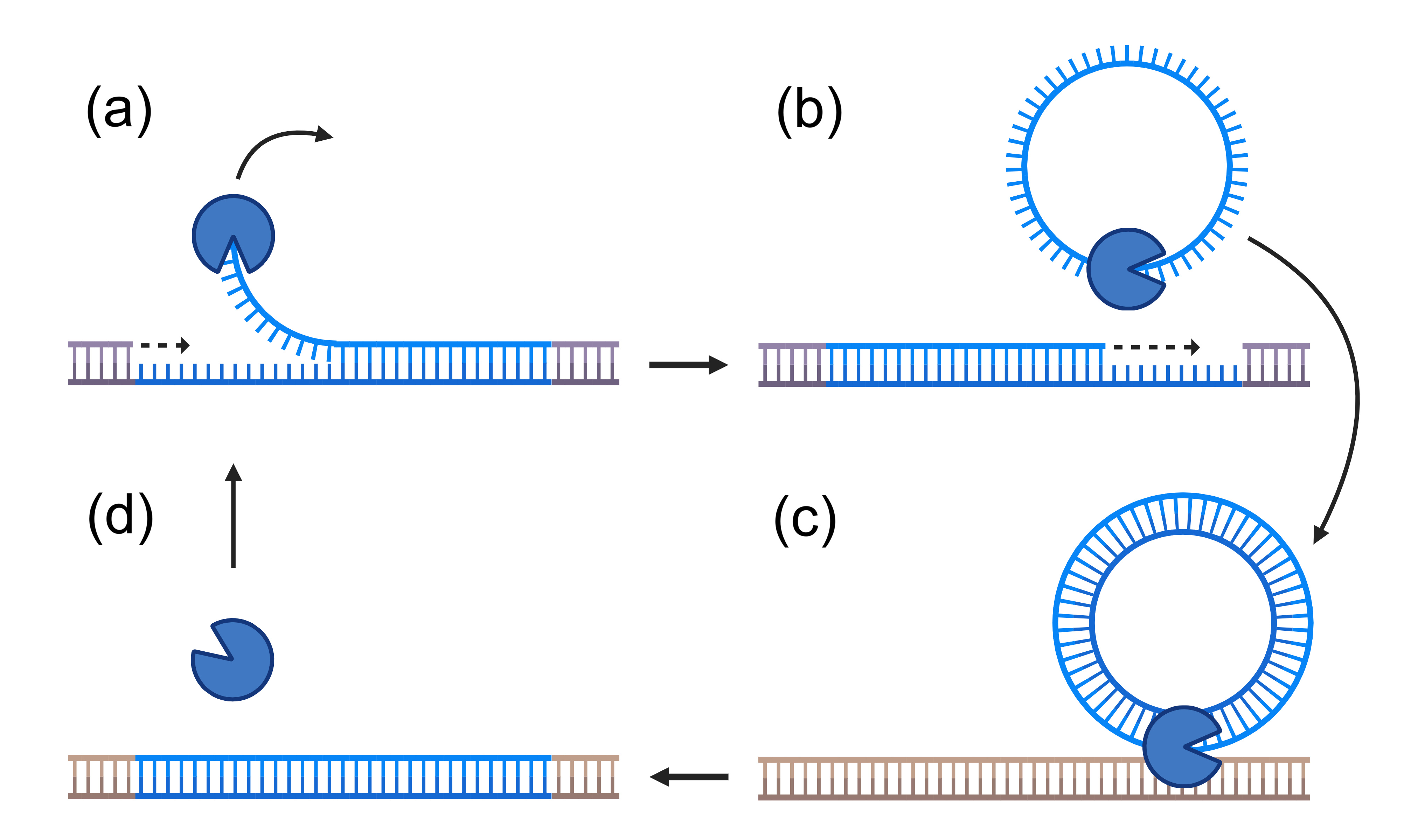
Helitrons have a simple life cycle (Figure 1, reviewed in Refs. [2, 20]), wherein they utilize a transposase protein to replicate themselves. Autonomous helitrons produce this protein, while non-autonomous helitrons use whatever transposase they can obtain. Upon binding to the helitron, the transposase copies the helitron DNA sequence and inserts this copy elsewhere into the genome, potentially harming the host. Crucially, this process requires only one transposase, so the mean transposition rate should scale linearly with the transposase concentration, at least up to a point. This contrasts with other transposon species which may require complexes of two or more transposases to replicate.
Including sex, there are four processes for which any model of transposon populations must account:
-
1.
Sex
-
2.
Transposition
-
3.
Transpositional toxicity
-
4.
Transposon loss
In the sections that follow, we derive the effects of each of these four processes on the distribution of transposons in our host species. We will take the host population to be infinite until Section III.4, wherein we analyze finite size effects. For simplicity, we assume that mating is panmictic and occurs much more frequently than the per element rate of transposition, which appears to be the case for many real-life transposons in equilibrium [24, 25, 26, 27, 28, 29]. The effects of toxicity and loss are also taken to be small, as is typically the case in nature [30, 31, 32, 33].
We define a strain to be a population of transposons with a defined set of parameters , , and , which characterize its propensity to replicate, to produce transposase, and to be lost from the genome, respectively. We analyze ecosystems of many interacting strains, but we do not consider events wherein one strain mutates into another.
We shall conclude this section by deriving an equation for the complete dynamics of transposon populations in our model. Let us therefore begin by computing the effect of each of these subprocesses on the mean transposon count.
II.1 Sex
Let be a random variable denoting the number of elements of strain in a randomly chosen host. So long as the population is in linkage equilibrium, which occurs whenever mating is frequent and panmictic, will be Poissonian [14]. It follows that we may compute the entire evolution of the helitron distribution simply by accounting for changes in the mean . Random mating of course has no effect on , so let us consider processes which do.
II.2 Transposition
We assume here that each strain in this ecosystem replicates at a rate proportional to and produces transposase at a rate . The sum quantifies the total amount of transposase being produced within the cell, and acts as a background field stimulating the replication of helitrons. The probability of replication for a strain is thus given by , where we have introduced the functional response to account for the reduction in transposition which occurs when elements must compete for a limited amount of transposase.
In our model, we take the functional response to be Holling’s type II, , although the precise form of this function is not important. What matters is that it decays like , which should be true of any model, since at some point the replication rate must be bounded by the availability of free transposase or another resource. This response function also happens to be equivalent to assuming Michaelis-Menten kinetics for the transposon-transposase reaction. Without loss of generality, we may absorb the constants into and , to get . Let us now proceed to calculate the change in the mean transposon count :
where we have defined , , and assumed , which is true so long as the total transposon activity eclipses the activity of any single element in the cell. The brackets denote the Poisson expectation value. Note that this approximation is valid because for large , and because we expect the mean number of helitrons per host to be large [34, 35, 36, 37]. We shall use this approximation with abandon throughout our analysis.
II.3 Transpositional toxicity
Helitrons place a fitness burden on their hosts in the process of transposition. Let us suppose that when the transposon replicates, it may kill the host with some probability . Using the same approximations as before, we may compute the mean effect on transposon populations:
One may also wonder whether the helitron places some fitness burden on its host even when it is not replicating. In that case, we would take the toxicity to be proportional to the number of helitrons and get . As we shall see, such a term can simply be absorbed into the term for transposon loss.
II.4 Transposon loss
Finally, we consider the effects of genetic drift and transposon deletion on helitron populations. Since each element has some rate of decaying or being lost in each generation, the effect on will be:
II.5 Total mean change in transposon count
Having considered in detail the individual effects of each of these processes, we may now obtain the total mean change in transposon count:
where we have replaced with since this will serve as our model for the rest of this paper. This equation is valid so long as and and are small.
III Results
III.1 Stable ecosystems consist of one autonomous and one non-autonomous strain
When do transposon strains coexist in equilibrium in our model? So long as we are not interested in timescales, we may reparametrize our model such that . Our equations then simplify to a generalized Lotka-Volterra model:
If all strains are non-autonomous (), then there will be no transposase production, and all elements will go extinct. However, if for all strains , then since and are small, , and will diverge. As grows, the toxicity of the helitrons will eventually lead to the collapse of the host population. Therefore, stable populations must consist of at least one autonomous and one non-autonomous strain.
We now proceed to show that, except on a measure-zero subset of our parameter space, stable populations will always consist of precisely one autonomous and one non-autonomous strain. Let us consider the long-time behavior of orbits by defining the long-time averages and . For any stable strain, will average to zero over the long term. Thus:
For these linear equations to yield a solution , the vectors must all lie on the same plane. This is not possible without fine-tuning for strains. It follows that stable ecosystems should consist of exactly one autonomous and one non-autonomous strain. This can be observed in simulations of our model (Figure 2), wherein less fit strains are whittled away until only one autonomous and one non-autonomous strain remain.
III.2 Coexistence collapses when
Having shown that stable orbits consist of one autonomous and one non-autonomous strain, we now restrict our attention to the following two-strain model:
where and denote autonomy and non-autonomy, and where we have taken , which can be done without loss of generality by rescaling , , . Note that this operation makes all of our parameters dimensionless.
The fixed point of these equations occurs at:
where we have again employed the approximation .
Since , this fixed point only exists when . The existence of a fixed point is our first requirement for coexistence. We must now assess the stability of this fixed point. It is easy to linearize our equations about their fixed point and find the eigenvalues, . The fixed point is stable when the real parts of these eigenvalues are all negative, which occurs if and only if . To summarize:
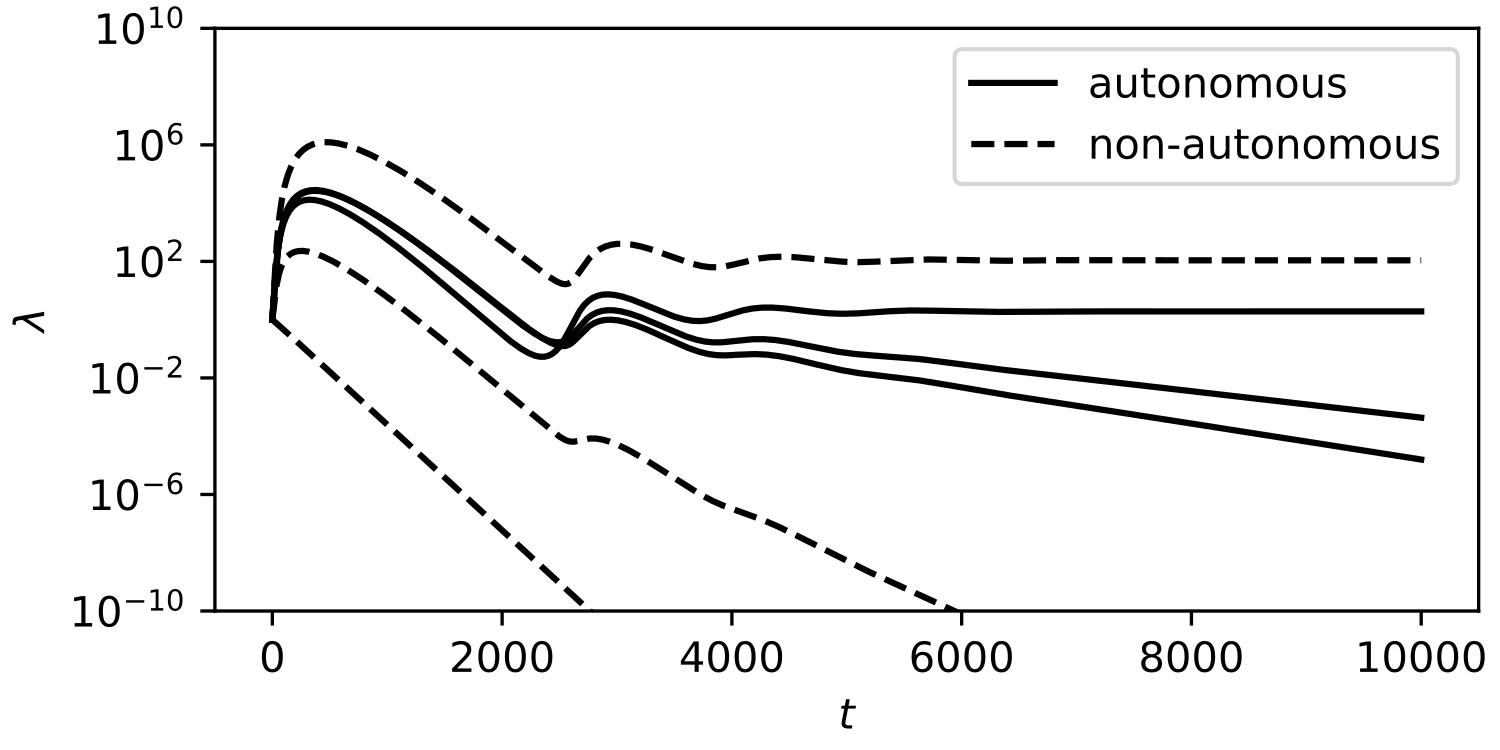
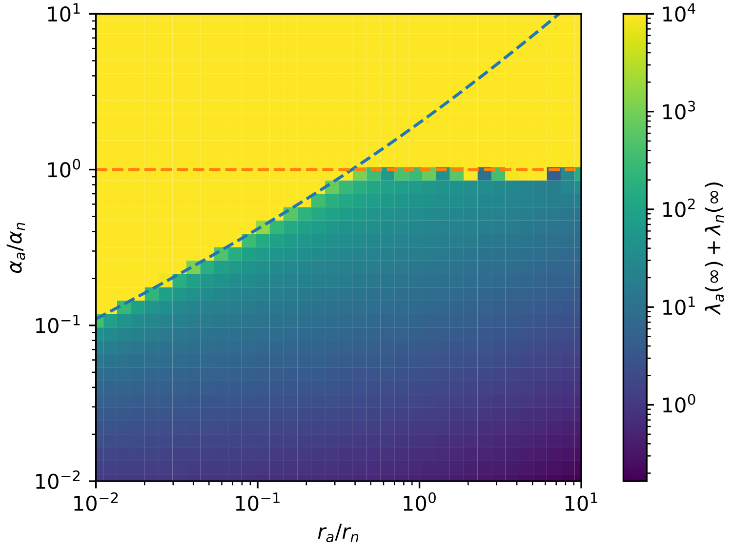
We illustrate the transition from stable coexistence to diverging/collapsing orbits in Figure 3. It is worth noting that because autonomous elements have more potential points of failure and are more problematic for the cell, we should expect . We may also imagine that the deleteriousness of the helitron is more significant than its decay rate, leading to . Either of these conditions will imply that whenever , the model automatically satisfies . Thus for real life helitrons, is probably the only relevant phase boundary.
III.3 Low transposition rates and few autonomous elements in equilibrium
Taking the ratio of and , we can see that autonomous elements come to be greatly outnumbered by their non-autonomous partners in equilibrium:
As a result, the per element transposition rate becomes low near the fixed point:
III.4 Finite population effects
What happens when the number of hosts is finite? In this case, the randomness of events like mating cannot be neglected, and the evolution of becomes stochastic. Our system may therefore be described by a multidimensional Fokker-Planck equation whose drift term comes from our equations for and whose diffusion term we may compute from the variances of each of the four subprocesses in our model.
Near the fixed point, the only non-negligible contribution to the variance comes from random mating, which contributes a factor of per generation. As our populations approach equilibrium, the distribution becomes approximately normal, centered about , with variance . We may solve for using the Lyapunov equation:
where , , and denotes the number for generations per unit time, which we may take to be without loss of generality.
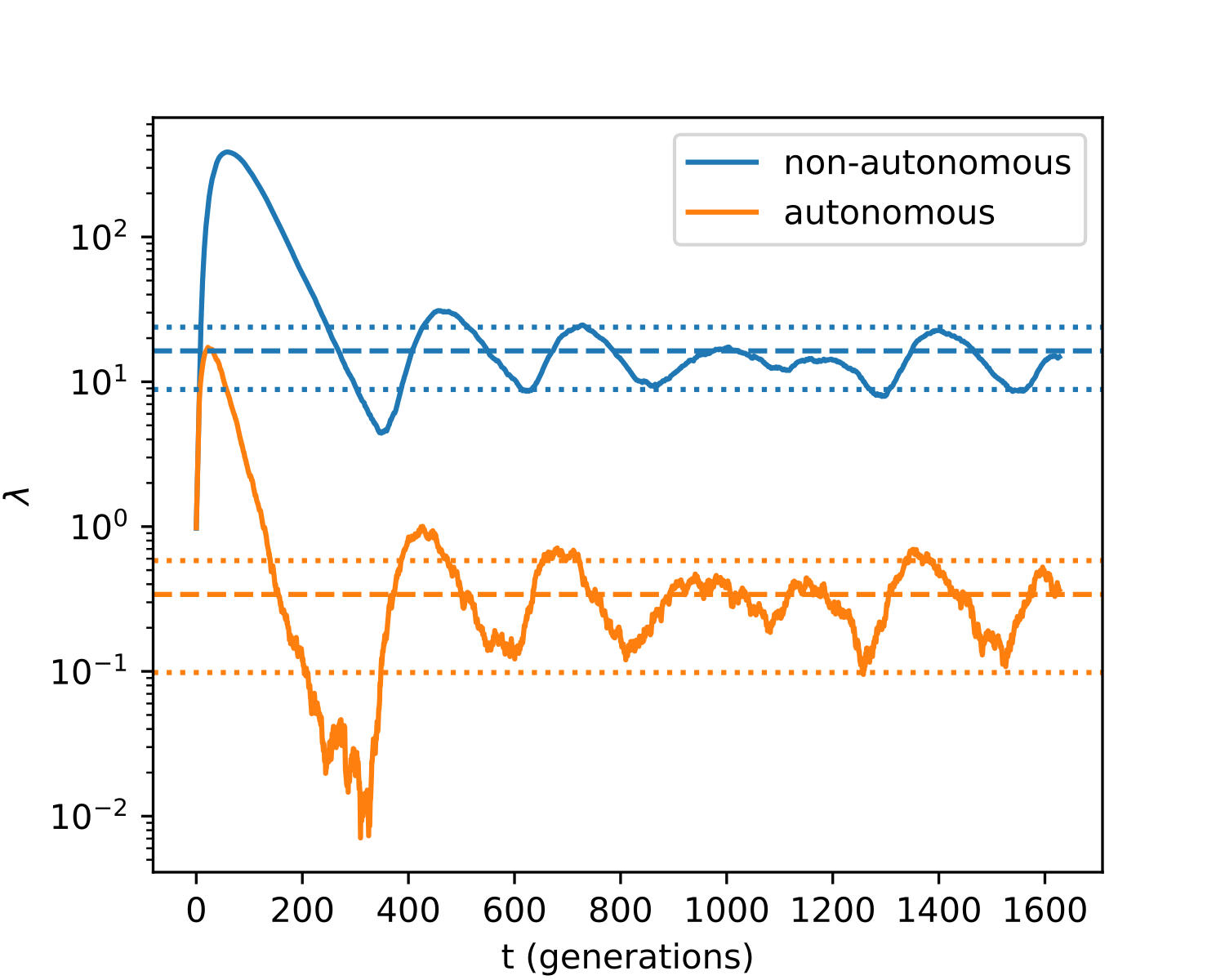
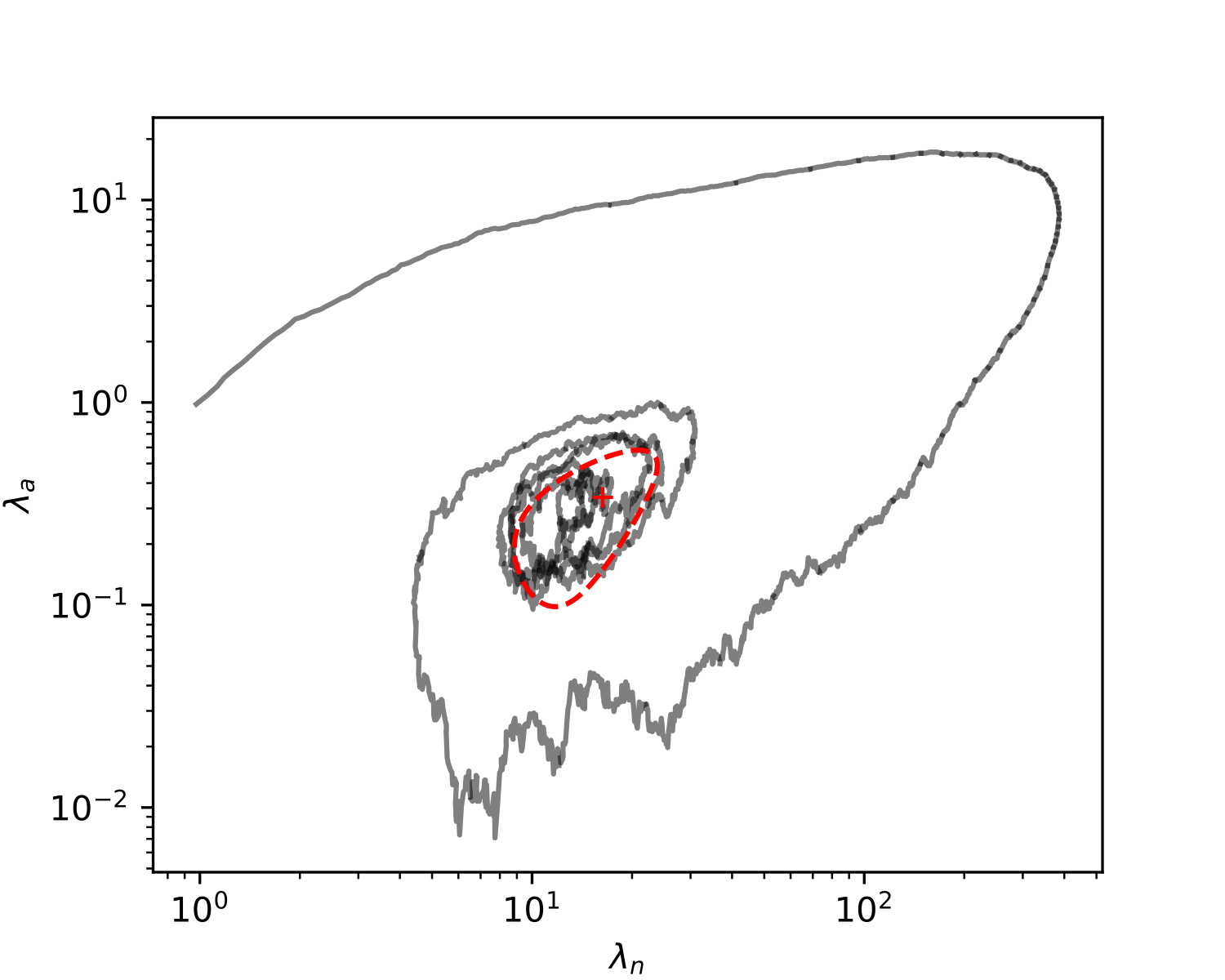
Figure 4 illustrates a sample trajectory from our model. We can see that even for relatively small populations (), orbits converge to the expected equilibria, and our estimates for the fluctuation sizes are accurate as well.
IV Discussion
IV.1 Stability in Class I and instability in Class II models
We are now in a position to understand why previous Class II models tended towards instability. In each of these models [12, 13, 14, 15, 16], the replication rates were taken to be proportional to the transposase concentration, placing them into the same framework analyzed herein. But in each of these models, the parameters and were taken to be equal for simplicity. Unfortunately, by taking , past researchers placed their populations precisely on the phase boundary between coexistence and collapse. Hence, the instability.
What can we say about the stable equilibrium found in Ref. [17] for long and short interspersed nuclear elements (LINEs and SINEs), a common pair of autonomous and non-autonomous Class I elements? To simplify their model to its mean-field essence, their equations were roughly of the form:
These equations differ from ours in two important ways: (a) they have no functional response, and (b) the autonomous transposition rate is not proportional to . It is the latter difference which accounts for the stability of these equations, since the analogous transposition parameters, and , do not have a constant ratio. Therefore, if populations begin to diverge, they will eventually reach a regime wherein , and the system will self-stabilize.
The essential difference between this model and ours arises from the fact that in the LINE replication process, the transposase is imagined to bind immediately to the LINE transcript which generates it, rather than binding to a random element in the DNA [42, 43]. This is known as “cis-preference” and occurs in some other Class I elements as well, but does not occur in Class II elements [44, 45]. It follows that cis-binding Class I ecosystems should be stable, while Class II ecosystems may be stable or unstable.
IV.2 Predictions of the model
Aside from the coexistence or collapse of helitron populations, our model also makes the following two quantitative predictions:
-
(i)
That non-autonomous elements should outnumber autonomous ones, at least in equilibrium.
-
(ii)
That per element transposition rates should be low in stable populations.
Our first prediction, although it may seem counterintuitive, has been confirmed numerous times [36, 34, 2]. Heuristic arguments for the fitness advantage of non-autonomous elements over autonomous ones have been given by many previous authors (see [10] for example). If our results are correct, then we have derived the first formula to quantify this preponderance.
Our second prediction, that per element transposition rates should be low, has been verified in helitrons and many other transposons [24, 25, 26, 27, 28, 29]. One explanation for this phenomenon could be that hosts have evolved to suppress transposons, but if this is the case, then why haven’t hosts been able to suppress viruses to a similar extent? The threat posed by viruses is far greater, yet their replication rates remain many orders of magnitude higher. In our model, we show instead that transposons can be kept in check by other transposons rather than by the host.
Do these results hold for transposons other than helitrons? Let us consider the aforementioned case of LINEs and SINEs, which together occupy one third of the human genome [4]. Since active SINEs outnumber LINEs at least ten to one, they clearly satisfy (i) [39, 41]. And since both elements transpose on the order of once per hundred generations, amounting some replications per active element per generation, they also satisfy (ii) [38, 40]. Therefore, these results may be much more universal than one may expect from this simple model.
IV.3 Concluding remarks
Can this model explain the survival or collapse of real-life transposon populations? This question is difficult to answer, as the relevant parameters for natural populations have not been measured. However, since is essentially a measure transposase affinity, one could perform an experiment to test our criterion in any number of transposon species and compare the results to natural populations.
In this article, we derived some simple equations for the stability and properties of transposon ecosystems which appear to explain the behavior of diverse transposon species. In particular, we have shown how subtle parameter changes can cause transposon populations to diverge dramatically, which could shed light on why similar species can have vastly different genome sizes, the so-called ”c-value enigma” (footnote 111A complete discussion of the c-value enigma would be beyond the scope of this article. It will suffice to say that the sizes of Eukaryotic genomes can vary widely, and often bear little relation to the supposed complexity of the organism or to closely related species. This variation is accounted for by differences in the amount of non-coding DNA between species, a large fraction of which can be attributed to transposons, yet little is known about why transposon populations in similar species can differ by orders of magnitude.). Transposons are an ancient part of life on Earth, and are the most abundant elements of our genomes. Thus, in studying these tiny organisms, we learn of life’s aeons, and of ourselves.
All code used to generate our plots is freely available at github.com/moyja/transposon_paper
Acknowledgements.
This work was supported in part with funding from NIGMS (R35 GM119850).Appendix A On superlinear toxicities
Consider a single transposon which replicates at a rate and which causes the host to perish at a rate . In this case, the mean rate of change in transposon count will be . Since such a model admits no nonzero equilibrium, we may be inclined to introduce a nonlinear term to the toxicity, resulting in the following equation:
This simple approach was advocated in the earliest models for transposon population dynamics to ensure the existence of a stable equilibrium population, and has continued to be used in more recent studies as well [47, 48, 15, 16]. However, in order to obtain such a term, there must be some mechanism by which the transposon toxicity compounds more than linearly in . Such a mechanism can either be transposition-dependent or transposition-independent.
The former case includes effects like insertional mutagenesis. Conceivably perhaps, the transposition of two elements in close succession could kill the host with high probability, while a single transposition would not. But as we mentioned earlier, the most abundant transposons in the human genome replicate just once per thousand years [38, 40]. It is therefore difficult to imagine how any such interaction could occur.
The latter case includes effects like ectopic recombination, which was once the most popular hypothesis to explain this phenomenon [49, 50]. In this case it is imagined that the presence of transposons in the genome may disrupt the DNA recombination machinery and lead to fatal errors in crossing over. This view is articulated in Ref. [13]:
“A balance between transposition and selection can be achieved, but only if the logarithm of the fitness of an individual with copies of a transposable element declines more than linearly with . This selection could arise through ectopic recombination with the transposable elements acting as scattered sites of homology in the chromosomes. The frequencies of such events will increase with the square of transposable element copy number… One interesting aspect is that the selection arises purely because these sequences are interspersed repetitive, and not because of any transposition process which they are undergoing.”
There is ample evidence that transposons do indeed cause ectopic recombination, but this only implies a nonzero contribution to [51, 52]. In order to gain insight into the contribution of ectopic exchange or of any other transposition-independent mechanism to , let us consider the case of transposition-incompetent elements.
Though our genomes are saturated with transposons, the vast majority of them are no longer capable of transposition, having lost or damaged sequences critical to their replication [53, 54, 55, 56, 18, 57, 11, 35]. If these “dead” transposons posed a meaningful threat to host fitness, then we would expect to see them quickly removed from the population. Their “live” cousins may also be deleterious, but at least they have the capacity to replicate to offset this shortcoming, and they should therefore be fitter and more abundant than their transposition-incompetent counterparts.
To make this argument more mathematically precise, let us decompose our simple model into “live” and “dead” populations:
| (1) | ||||
| (2) |
If , we may neglect its quadratic contribution to the term, leaving us again with a linear differential equation with no equilibrium. Furthermore, since , the dead transposons will be whittled out of the population. Thus, the transposition-independent hypothesis is not consistent with the observed preponderance of transposition-incompetent elements.
Finally in all of these models, we would expect transposons to want to evolve to ever increasing replication rates, which would appear to be possible by comparison with viral replication rates, but instead we tend to see very low transposon replication rates [24, 25, 26, 27, 28, 29]. On all of these grounds, we must reject the notion that nonlinear toxicities are relevant to stabilizing transposon populations.
References
- Siguier et al. [2014] P. Siguier, E. Gourbeyre, and M. Chandler, Bacterial insertion sequences: their genomic impact and diversity, FEMS Microbiology Reviews 38, 865 (2014), https://academic.oup.com/femsre/article-pdf/38/5/865/18142951/38-5-865.pdf .
- Thomas and Pritham [2015] J. Thomas and E. J. Pritham, Helitrons, the eukaryotic rolling-circle transposable elements, Microbiology Spectrum 3, 10.1128/microbiolspec.mdna3 (2015), https://journals.asm.org/doi/pdf/10.1128/microbiolspec.mdna3-0049-2014 .
- Wells and Feschotte [2020] J. Wells and C. Feschotte, A field guide to eukaryotic transposable elements, Annu Rev Genet 54, 539 (2020), pMID: 32955944.
- Lander et al. [2001] E. Lander, L. Linton, B. Birren, C. Nusbaum, M. Zody, J. Baldwin, K. Devon, K. Dewar, M. Doyle, W. FitzHugh, R. Funke, D. Gage, K. Harris, A. Heaford, J. Howland, L. Kann, J. Lehoczky, R. LeVine, P. McEwan, K. McKernan, J. Meldrim, J. Mesirov, C. Miranda, W. Morris, J. Naylor, C. Raymond, M. Rosetti, R. Santos, A. Sheridan, C. Sougnez, Y. Stange-Thomann, N. Stojanovic, A. Subramanian, D. Wyman, J. Rogers, J. Sulston, R. Ainscough, S. Beck, D. Bentley, J. Burton, C. Clee, N. Carter, A. Coulson, R. Deadman, P. Deloukas, A. Dunham, I. Dunham, R. Durbin, L. French, D. Grafham, S. Gregory, T. Hubbard, S. Humphray, A. Hunt, M. Jones, C. Lloyd, A. McMurray, L. Matthews, S. Mercer, S. Milne, J. Mullikin, A. Mungall, R. Plumb, M. Ross, R. Shownkeen, S. Sims, R. Waterston, R. Wilson, L. Hillier, J. McPherson, M. Marra, E. Mardis, L. Fulton, A. Chinwalla, K. Pepin, W. Gish, S. Chissoe, M. Wendl, K. Delehaunty, T. Miner, A. Delehaunty, J. Kramer, L. Cook, R. Fulton, D. Johnson, P. Minx, S. Clifton, T. Hawkins, E. Branscomb, P. Predki, P. Richardson, S. Wenning, T. Slezak, N. Doggett, J. Cheng, A. Olsen, S. Lucas, C. Elkin, E. Uberbacher, M. Frazier, R. Gibbs, D. Muzny, S. Scherer, J. Bouck, E. Sodergren, K. Worley, C. Rives, J. Gorrell, M. Metzker, S. Naylor, R. Kucherlapati, D. Nelson, G. Weinstock, Y. Sakaki, A. Fujiyama, M. Hattori, T. Yada, A. Toyoda, T. Itoh, C. Kawagoe, H. Watanabe, Y. Totoki, T. Taylor, J. Weissenbach, R. Heilig, W. Saurin, F. Artiguenave, P. Brottier, T. Bruls, E. Pelletier, C. Robert, P. Wincker, D. Smith, L. Doucette-Stamm, M. Rubenfield, K. Weinstock, H. Lee, J. Dubois, A. Rosenthal, M. Platzer, G. Nyakatura, S. Taudien, A. Rump, H. Yang, J. Yu, J. Wang, G. Huang, J. Gu, L. Hood, L. Rowen, A. Madan, S. Qin, R. Davis, N. Federspiel, A. Abola, M. Proctor, R. Myers, J. Schmutz, M. Dickson, J. Grimwood, D. Cox, M. Olson, R. Kaul, C. Raymond, N. Shimizu, K. Kawasaki, S. Minoshima, G. Evans, M. Athanasiou, R. Schultz, B. Roe, F. Chen, H. Pan, J. Ramser, H. Lehrach, R. Reinhardt, W. McCombie, M. de la Bastide, N. Dedhia, H. Blöcker, K. Hornischer, G. Nordsiek, R. Agarwala, L. Aravind, J. Bailey, A. Bateman, S. Batzoglou, E. Birney, P. Bork, D. Brown, C. Burge, L. Cerutti, H. Chen, D. Church, M. Clamp, R. Copley, T. Doerks, S. Eddy, E. Eichler, T. Furey, J. Galagan, J. Gilbert, C. Harmon, Y. Hayashizaki, D. Haussler, H. Hermjakob, K. Hokamp, W. Jang, L. Johnson, T. Jones, S. Kasif, A. Kaspryzk, S. Kennedy, W. Kent, P. Kitts, E. Koonin, I. Korf, D. Kulp, D. Lancet, T. Lowe, A. McLysaght, T. Mikkelsen, J. Moran, N. Mulder, V. Pollara, C. Ponting, G. Schuler, J. Schultz, G. Slater, A. Smit, E. Stupka, J. Szustakowki, D. Thierry-Mieg, J. Thierry-Mieg, L. Wagner, J. Wallis, R. Wheeler, A. Williams, Y. Wolf, K. Wolfe, S. Yang, R. Yeh, F. Collins, M. Guyer, J. Peterson, A. Felsenfeld, K. Wetterstrand, A. Patrinos, M. Morgan, P. de, Jong, J. Catanese, K. Osoegawa, H. Shizuya, S. Choi, Y. Chen, and J. Szustakowki, Initial sequencing and analysis of the human genome, Nature 409(6822), 860 (2001), pMID: 11237011.
- Kazazian et al. [1988] J. Kazazian, HH, C. Wong, H. Youssoufian, A. Scott, D. Phillips, and S. Antonarakis, Haemophilia a resulting from de novo insertion of l1 sequences represents a novel mechanism for mutation in man, Nature 332(6160), 164 (1988), pMID: 2831458.
- Pradhan and Ramakrishna [2022] R. K. Pradhan and W. Ramakrishna, Transposons: Unexpected players in cancer, Gene 808, 145975 (2022).
- Prak and Kazazian [2000] E. Prak and H. J. Kazazian, Mobile elements and the human genome, Nat Rev Genet 1(2), 134 (2000), pMID: 11253653.
- Havecker et al. [2004] E. Havecker, X. Gao, and D. Voytas, The diversity of ltr retrotransposons, Genome Biol 5(6), 225 (2004), pMID: 15186483.
- Venkatesh and Nandini [2020] Venkatesh and B. Nandini, Miniature inverted-repeat transposable elements (mites), derived insertional polymorphism as a tool of marker systems for molecular plant breeding, Mol Biol Rep 47(4), 3155 (2020), pMID: 32162128.
- Leonardo and Nuzhdin [2002] T. Leonardo and S. Nuzhdin, Intracellular battlegrounds: conflict and cooperation between transposable elements, Genet Res 80(3), 155 (2002), pMID: 12688654.
- Brookfield [2005] J. Brookfield, The ecology of the genome - mobile dna elements and their hosts, Nat Rev Genet 6(2), 128 (2005), pMID: 15640810.
- Kaplan et al. [1985] N. Kaplan, T. Darden, and C. Langley, Evolution and extinction of transposable elements in mendelian populations, Genetics 109(2), 459 (1985), pMID: 2982700.
- Brookfield [1991] J. Brookfield, Models of repression of transposition in p-m hybrid dysgenesis by p cytotype and by zygotically encoded repressor proteins, Genetics 128(2), 471 (1991), pMID: 1649073.
- Brookfield [1996] J. Brookfield, Models of the spread of non-autonomous selfish transposable elements when transposition and fitness are coupled, Genetics Research 67(3), 199 (1996).
- Le and Capy [2006] A. Le, Rouzic and P. Capy, Population genetics models of competition between transposable element subfamilies, Genetics 174(2), 785 (2006), pMID: 16888345.
- Le et al. [2007] A. Le, Rouzic, T. Boutin, and P. Capy, Long-term evolution of transposable elements, Proc Natl Acad Sci U S A 104(49), 19375 (2007), pMID: 200.
- Xue and Goldenfeld [2016] C. Xue and N. Goldenfeld, Stochastic predator-prey dynamics of transposons in the human genome, Phys Rev Lett 117(20), 208101 (2016), pMID: 27886494.
- Feschotte et al. [2002] C. Feschotte, N. Jiang, and S. Wessler, Plant transposable elements: where genetics meets genomics, Nat Rev Genet 3(5), 329 (2002), pMID: 11988759.
- Oggenfuss et al. [2021] U. Oggenfuss, T. Badet, T. Wicker, F. E. Hartmann, N. K. Singh, L. Abraham, P. Karisto, T. Vonlanthen, C. Mundt, B. A. McDonald, and D. Croll, A population-level invasion by transposable elements triggers genome expansion in a fungal pathogen, eLife 10, e69249 (2021).
- Barro-Trastoy and Köhler [2024] D. Barro-Trastoy and C. Köhler, Helitrons: genomic parasites that generate developmental novelties, Trends Genet 40(5), 437 (2024), pMID: 38429198.
- Grabundzija et al. [2016] I. Grabundzija, S. Messing, J. Thomas, R. Cosby, I. Bilic, C. Miskey, A. Gogol-Döring, V. Kapitonov, T. Diem, A. Dalda, J. Jurka, E. Pritham, F. Dyda, Z. Izsvák, and Z. Ivics, A helitron transposon reconstructed from bats reveals a novel mechanism of genome shuffling in eukaryotes, Nat Commun 7, 10716 (2016), pMID: 26931494.
- Grabundzija et al. [2018] I. Grabundzija, A. Hickman, and F. Dyda, Helraiser intermediates provide insight into the mechanism of eukaryotic replicative transposition, Nat Commun 9(1), 1278 (2018), pMID: 29599430.
- Chakrabarty et al. [2023] P. Chakrabarty, R. Sen, and S. Sengupta, From parasites to partners: exploring the intricacies of host-transposon dynamics and coevolution, Funct Integr Genomics 23(3), 278 (2023), pMID: 37610667.
- Shen et al. [1987] M. Shen, E. Raleigh, and N. Kleckner, Physical analysis of tn10- and is10-promoted transpositions and rearrangements, Genetics 116(3), 359 (1987), pMID: 3038673.
- Harada et al. [1990] K. Harada, K. Yukuhiro, and T. Mukai, Transposition rates of movable genetic elements in drosophila melanogaster, Proc Natl Acad Sci U S A 87(8), 3248 (1990), pMID: 2158108.
- Nuzhdin and Mackay [1994] S. Nuzhdin and T. Mackay, Direct determination of retrotransposon transposition rates in drosophila melanogaster, Genet Res 63(2), 139 (1994), pMID: 8026740.
- Suh et al. [1995] D. Suh, E. Choi, T. Yamazaki, and K. Harada, Studies on the transposition rates of mobile genetic elements in a natural population of drosophila melanogaster, Mol Biol Evol 12(5), 748 (1995), pMID: 7476122.
- Maside et al. [2000] X. Maside, S. Assimacopoulos, and B. Charlesworth, Rates of movement of transposable elements on the second chromosome of drosophila melanogaster, Genet Res 75(3), 275 (2000), pMID: 10893864.
- Sousa et al. [2013] A. Sousa, C. Bourgard, L. Wahl, and I. Gordo, Rates of transposition in escherichia coli, Biol Lett 9(6), 20130838 (2013), pMID: 24307531.
- Eanes et al. [1988] W. F. Eanes, C. Wesley, J. Hey, D. Houle, and J. W. Ajioka, The fitness consequences of p element insertion in drosophila melanogaster, Genetics Research 52, 17–26 (1988).
- Charlesworth and Langley [1989] B. Charlesworth and C. Langley, The population genetics of drosophila transposable elements, Annu Rev Genet 23, 251 (1989), pMID: 2559652.
- Houle and Nuzhdin [2004] D. Houle and S. V. Nuzhdin, Mutation accumulation and the effect of copia insertions in drosophila melanogaster, Genetics Research 83, 7 (2004).
- Pasyukova et al. [2004] E. Pasyukova, S. Nuzhdin, T. Morozova, and T. Mackay, Accumulation of transposable elements in the genome of drosophila melanogaster is associated with a decrease in fitness, Journal of Heredity 95, 284 (2004).
- Yang and Bennetzen [2009a] L. Yang and J. L. Bennetzen, Structure-based discovery and description of plant and animal ¡i¿helitrons¡/i¿, Proceedings of the National Academy of Sciences 106, 12832 (2009a), https://www.pnas.org/doi/pdf/10.1073/pnas.0905563106 .
- Yang and Bennetzen [2009b] L. Yang and J. L. Bennetzen, Distribution, diversity, evolution, and survival of ¡i¿helitrons¡/i¿ in the maize genome, Proceedings of the National Academy of Sciences 106, 19922 (2009b), https://www.pnas.org/doi/pdf/10.1073/pnas.0908008106 .
- Du et al. [2009] C. Du, N. Fefelova, J. Caronna, L. He, and H. K. Dooner, The polychromatic ¡i¿helitron¡/i¿ landscape of the maize genome, Proceedings of the National Academy of Sciences 106, 19916 (2009), https://www.pnas.org/doi/pdf/10.1073/pnas.0904742106 .
- Xiong et al. [2014] W. Xiong, L. He, J. Lai, H. K. Dooner, and C. Du, Helitronscanner uncovers a large overlooked cache of ¡i¿helitron¡/i¿ transposons in many plant genomes, Proceedings of the National Academy of Sciences 111, 10263 (2014), https://www.pnas.org/doi/pdf/10.1073/pnas.1410068111 .
- Cordaux et al. [2006] R. Cordaux, D. J. Hedges, S. W. Herke, and M. A. Batzer, Estimating the retrotransposition rate of human alu elements, Gene 373, 134 (2006).
- Bennett et al. [2008] E. Bennett, H. Keller, R. Mills, S. Schmidt, J. Moran, O. Weichenrieder, and S. Devine, Active alu retrotransposons in the human genome, Genome Res 18(12), 1875 (2008), pMID: 18836035.
- Xing et al. [2009] J. Xing, Y. Zhang, K. Han, A. Salem, S. Sen, C. Huff, Q. Zhou, E. Kirkness, S. Levy, M. Batzer, and L. Jorde, Mobile elements create structural variation: analysis of a complete human genome, Genome Res 19(9), 1516 (2009), pMID: 19439515.
- Beck et al. [2011] C. Beck, J. Garcia-Perez, R. Badge, and J. Moran, Line-1 elements in structural variation and disease, Annu Rev Genomics Hum Genet 12, 187 (2011), pMID: 21801021.
- Esnault et al. [2000] C. Esnault, J. Maestre, and T. Heidmann, Human line retrotransposons generate processed pseudogenes, Nat Genet 24(4), 363 (2000), pMID: 10742098.
- Wei et al. [2001] W. Wei, N. Gilbert, S. L. Ooi, J. F. Lawler, E. M. Ostertag, H. H. Kazazian, J. D. Boeke, and J. V. Moran, Human l1 retrotransposition: cis preference versus trans complementation, Molecular and Cellular Biology 21, 1429 (2001), pMID: 11158327, https://doi.org/10.1128/MCB.21.4.1429-1439.2001 .
- Bolton et al. [2005] E. Bolton, C. Coombes, Y. Eby, M. Cardell, and J. Boeke, Identification and characterization of critical cis-acting sequences within the yeast ty1 retrotransposon, RNA 11(3), 308 (2005), pMID: 15661848.
- Curcio et al. [2015] M. J. Curcio, S. Lutz, and P. Lesage, The ty1 ltr-retrotransposon of budding yeast, ¡i¿saccharomyces cerevisiae¡/i¿, Microbiology Spectrum 3, 10.1128/microbiolspec.mdna3 (2015), https://journals.asm.org/doi/pdf/10.1128/microbiolspec.mdna3-0053-2014 .
- Note [1] A complete discussion of the c-value enigma would be beyond the scope of this article. It will suffice to say that the sizes of Eukaryotic genomes can vary widely, and often bear little relation to the supposed complexity of the organism or to closely related species. This variation is accounted for by differences in the amount of non-coding DNA between species, a large fraction of which can be attributed to transposons, yet little is known about why transposon populations in similar species can differ by orders of magnitude.
- Brookfield [1982] J. Brookfield, Interspersed repetitive dna sequences are unlikely to be parasitic, J Theor Biol 94(2), 281 (1982), pMID: 7078209.
- Charlesworth and Charlesworth [1983] B. Charlesworth and D. Charlesworth, The population dynamics of transposable elements, Genetics Research 42(1), 1–27 (1983).
- Montgomery et al. [1987] E. Montgomery, B. Charlesworth, and C. Langley, A test for the role of natural selection in the stabilization of transposable element copy number in a population of drosophila melanogaster, Genet Res 49(1), 31 (1987), pMID: 3032743.
- Langley et al. [1988] C. Langley, E. Montgomery, R. Hudson, N. Kaplan, and B. Charlesworth, On the role of unequal exchange in the containment of transposable element copy number, Genet Res 52(3), 223 (1988), pMID: 2854088.
- Delprat et al. [2009] A. Delprat, B. Negre, M. Puig, and A. Ruiz, The transposon galileo generates natural chromosomal inversions in drosophila by ectopic recombination, PLoS One 4(11), e7883 (2009), pMID: 19936241.
- Santana et al. [2014] M. Santana, J. Silva, E. Mizubuti, E. Araújo, B. Condon, B. Turgeon, and M. Queiroz, Characterization and potential evolutionary impact of transposable elements in the genome of cochliobolus heterostrophus, BMC Genomics 15(1), 536 (2014), pMID: 24973942.
- Voliva et al. [1983] C. F. Voliva, C. L. Jahn, M. B. Comer, I. Hutchison, Clyde A., and M. H. Edgell, The L1Md long interspersed repeat family in the mouse: almost all examples are truncated at one end, Nucleic Acids Research 11, 8847 (1983), https://academic.oup.com/nar/article-pdf/11/24/8847/7048814/11-24-8847.pdf .
- Hardies et al. [1986] S. C. Hardies, S. L. Martin, C. F. Voliva, r. Hutchison, C A, and M. H. Edgell, An analysis of replacement and synonymous changes in the rodent L1 repeat family., Molecular Biology and Evolution 3, 109 (1986), https://academic.oup.com/mbe/article-pdf/3/2/109/11167308/2hard.pdf .
- Sassaman et al. [1997] D. Sassaman, B. Dombroski, J. Moran, M. Kimberland, T. Naas, R. DeBerardinis, A. Gabriel, G. Swergold, and H. J. Kazazian, Many human l1 elements are capable of retrotransposition, Nat Genet 16(1), 37 (1997), pMID: 9140393.
- Ostertag and Kazazian [2001] E. Ostertag and H. J. Kazazian, Twin priming: a proposed mechanism for the creation of inversions in l1 retrotransposition, Genome Res 11(12), 2059 (2001), pMID: 11731496.
- Brouha et al. [2003] B. Brouha, J. Schustak, R. Badge, S. Lutz-Prigge, A. Farley, J. Moran, and H. J. Kazazian, Hot l1s account for the bulk of retrotransposition in the human population, Proc Natl Acad Sci U S A 100(9), 5280 (2003), pMID: 12682288.