Phase Diagram of a Non-Hermitian Chern Insulator: Destabilization of Chiral Edge States and Bulk–Boundary Correspondence
Abstract
A non-Hermitian Chern insulator with gain/loss-type non-Hermiticity shows a peculiar gap closing; when a nontrivial Chern insulator phase changes to a gapless phase, conduction and valence bands are combined into one band owing to destabilization of chiral edge states. A previous recipe of non-Hermitian bulk–boundary correspondence is insufficient for this system since such a gap closing is beyond its scope. Here, we revise the recipe by taking the peculiar gap closing into account and apply it to the non-Hermitian Chern insulator. We demonstrate that the bulk–boundary correspondence holds in the system including a destabilization of chiral edge states. A phase diagram derived from the bulk–boundary correspondence is shown to be consistent with spectra of the system.
1 Introduction
Bulk–boundary correspondence is a characteristic feature that manifests itself in various topological systems. [1, 2, 3, 4, 5, 6, 7, 8, 9, 10] A topological number defined in bulk geometry under a periodic boundary condition (pbc) plays a central role in the original scenario of bulk–boundary correspondence proposed by Hatsugai [11] and Ryu and Hatsugai. [12] The topological number governs the presence or absence of topological boundary states in the boundary geometry under an open boundary condition (obc); if it is nontrivial (trivial), topological boundary states appear (disappear) in the boundary geometry. Note that the original scenario employs the bulk and boundary geometries.
Inspired by an extension of quantum mechanics to the non-Hermitian regime, [13, 14, 15] extensive studies have been conducted on non-Hermitian topological systems. [16, 17, 18, 19, 20, 21, 22, 23, 24, 25, 26, 27, 28, 29, 30, 31, 32, 33, 34, 35, 36, 37, 38, 39, 40, 41, 42, 43, 44, 45, 46, 47, 48, 49, 50, 51, 52, 53, 54, 55, 56, 57, 58, 59, 60, 61, 62, 63, 64, 65, 66, 67, 68, 69, 70, 71, 72, 73, 74, 75, 76, 77] Bulk–boundary correspondence is an important subject of these studies. It was demonstrated that a straightforward application of the original scenario fails to describe the topological nature of some non-Hermitian topological systems. [20, 24]
A reason for the breaking of the bulk–boundary correspondence is a non-Hermitian skin effect; [28, 78, 79, 80, 81, 82, 83, 84, 85, 86] eigenfunctions in a non-Hermitian system under the obc are localized near a boundary of the system. This effect is hidden in the system under the pbc. Indeed, all eigenfunctions under the pbc extend over the entire system. Therefore, a topological number defined in the bulk geometry under the pbc never reflects the non-Hermitian skin effect in the boundary geometry. Several scenarios without using the bulk geometry have been proposed. [28, 38, 27, 52] Although these scenarios can avoid difficulty concerning a non-Hermitian skin effect, they do not share the notable feature of the original scenario that a topological number defined in closed geometry governs the presence or absence of topological boundary states.
To restore the bulk–boundary correspondence in non-Hermitian topological systems, another scenario has been proposed in Refs. \citenimura1 and \citenimura2. This scenario employs boundary geometry under the obc and bulk geometry under a modified periodic boundary condition (mpbc). Let be a right eigenstate of a one-dimensional lattice system consisting of sites. The mpbc is defined by , where is a positive real constant. [47] The wavefunction satisfies this boundary condition when , where is the lattice constant. The case of corresponds to the ordinary pbc. If (), the mpbc selects wavefunctions that exponentially increase (decrease) with increasing . This behavior of resembles that caused by a non-Hermitian skin effect. Therefore, by using the bulk geometry under the mpbc, we can take the non-Hermitian skin effect into account in calculating a topological number.
The scenario in Refs. \citenimura1 and \citenimura2 succeeds in describing the bulk–boundary correspondence in one-dimensional non-Hermitian topological insulators. The present author [71] gave a recipe for executing the scenario in two-dimensional systems and applied it to a Chern insulator with gain/loss-type non-Hermiticity, [29] obtaining a phase diagram in the boundary geometry. The phase diagram separates three regions: a topologically nontrivial Chern insulator phase, a topologically trivial insulator phase, and a gapless phase. In Ref. \citentakane1, the phase boundary between the nontrivial and trivial regions and that between trivial and gapless regions are shown to be consistent with spectra in the boundary geometry. However, the phase boundary between the nontrivial and gapless regions is not fully consistent with spectra.
In this paper, we examine the bulk–boundary correspondence in the Chern insulator with gain/loss-type non-Hermiticity by using a revised recipe. A key observation is that the inconsistency reported in Ref. \citentakane1 is caused by a peculiar gap closing in the boundary geometry: if chiral edge states linking conduction and valence bands are destabilized by non-Hermiticity, the two bands are combined into one band without an obvious gap closing. This is beyond the scope of the recipe in Ref. \citentakane1. We thus revise the recipe of the bulk–boundary correspondence such that it can take the peculiar gap closing into account and show that the revised recipe enables us to describe the topological features of the system without any inconsistency. Indeed, we obtain a phase diagram that is fully consistent with spectra in the boundary geometry.
In the next section, we present a tight-binding Hamiltonian for the non-Hermitian Chern insulator with gain/loss-type non-Hermiticity [29] and specify two symmetries of it. Complex spectra of this system are constrained by these symmetries. In Sect. 3, we introduce right and left eigenstates of the Hamiltonian as a preparation for theoretical analyses. In Sect. 4, we consider chiral edge states in the geometry with the obc in one direction and the mpbc in the other direction. This consideration reveals important characteristics of chiral edge states in the boundary geometry, which are used in the following two sections. Section 5 is the central part of this paper. We give a revised recipe for executing the scenario of the bulk–boundary correspondence and obtain a phase diagram in the boundary geometry by using it. In Sect. 6, we justify the resulting phase diagram by comparing it with spectra of the system in the boundary geometry. The last section is devoted to a summary and discussion.
2 Model and Symmetries
We adopt a tight-binding model for non-Hermitian Chern insulators on a square lattice with lattice constant . The Hamiltonian is given by with [29]
| (1) | ||||
| (2) | ||||
| (3) |
where , , and are real parameters, and specify the location of each site in the - and -directions, and , , and are the -, -, and -components of Pauli matrices, respectively. and consist of spin-up and -down components:
| (5) | ||||
| (8) |
where and with , are, respectively. column and row vectors. If the number of sites in the system is , the column and row vectors consist of components, where the factor reflects the spin degrees of freedom. In and , only one component corresponding to the th site with is and other components are . They satisfy and
| (9) |
As a consequence, is a matrix. The Hamiltonian is normalized such that the coefficients of in and become and therefore is dimensionless. The non-Hermiticity of the system is characterized by . For simplicity, we focus on the case of and with throughout this paper. The model becomes topologically nontrivial when in the Hermitian limit of .
In the remainder of this section, we point out two symmetries that possesses. The first symmetry is
| (10) |
where acts on spin space. From this symmetry, we can show that, if satisfies , then satisfies . That is, an eigenstate of with an eigenvalue of is paired with its counterpart with the eigenvalue of if . The second symmetry is
| (11) |
where acts on spin space and represents the space inversion operator. If the system is square shaped with sites (i.e., ), then is expressed as
| (12) |
From this symmetry, we can show that, if satisfies , then satisfies . That is, an eigenstate of with an eigenvalue of is paired with its counterpart with the eigenvalue of if .
These results tell us that if an eigenstate with an eigenvalue of with and is present, this eigenstate and its three counterparts form a quartet: four eigenstates with , , , and are related by the two symmetries. An important exception is the case of and , where an eigenstate and its counterpart form a pair; eigenstates with and are related by the symmetries.
The above statement is useful in considering a complex spectrum of our system. Let us denote a complex eigenvalue of energy as . All eigenvalues are real as in the Hermitian limit of . With increasing , eigenvalues gradually become complex as ). We focus on a pair of eigenstates with eigenvalues of and at . Let us suppose that deviates from the real axis as with increasing . This statement requires that this eigenstate forms a quartet together with three other eigenstates with eigenvalues of , , and . Such a quartet should be formed by a combination of two pairs of eigenstates. That is, an eigenvalue can become complex only when a pair of eigenstates with and and another pair of eigenstates with and are degenerate in energy under the condition of .
3 Right and Left Eigenstates
We consider the system of sites in the boundary and bulk geometries. Right and left eigenstates of are expressed as
| (13) | |||
| (14) |
where and are, respectively, two component column and row vectors:
| (17) | ||||
| (19) |
In the boundary geometry, the following obc is imposed on and :
| (22) | ||||
| (24) |
In the bulk geometry, we introduce plane-wave-like right and left eigenstates to define a topological number. To do this, we set
| (25) | ||||
| (26) |
where and are, respectively, two component column and row vectors independent of and , and
| (27) | ||||
| (28) |
The eigenvalue equation is reduced to
| (29) |
where with
| (30) | ||||
| (31) | ||||
| (32) |
The eigenvalue equation is reduced to
| (33) |
where with
| (34) | |||
| (35) | |||
| (36) |
We impose the following mpbc on :
| (37) |
which results in
| (38) |
where and (). To present a biorthogonal set of right and left basis functions, [15] we determine and as
| (39) |
which results in
| (40) |
This indicates that obeys the following mpbc:
| (41) |
which is different from Eq. (37).
We find from Eq. (39) and thus denote them as hereafter. The reduced Hamiltonian is expressed as
| (42) |
with
| (43) | ||||
| (44) | ||||
| (45) |
where
| (46) |
By solving the reduced eigenvalue equation, we find that the energy of an eigenstate characterized by and is given by with
| (47) |
where . The right and left eigenstates of with the eigenvalue of are expressed as
| (48) | ||||
| (49) |
where
| (52) | ||||
| (55) |
with . We easily find
| (56) |
That is, and constitute a biorthogonal set of basis functions. [15] The eigenvectors satisfy
| (57) |
4 Chiral Edge States
We determine the spectrum of chiral edge states in the system when an obc is imposed in one direction and a mpbc is imposed in the other direction. Considering the resulting spectrum, we find important characteristics of chiral edge states in the boundary geometry.
First, we consider the system [see Fig. 1(a)] under the obc in the -direction,
| (58) |
and the mpbc in the -direction,
| (59) |
To obtain fundamental solutions, we set
| (60) |
where characterizes the penetration of chiral edge states in the -direction and . We decompose the reduced Hamiltonian as with
| (61) | ||||
| (62) |
where is given in Eq. (43) and
| (63) |
A simple method for obtaining edge localized solutions is described in Appendix of Ref. \citentakane2. By adapting the method to , we find two eigenstates at :
| (64) | ||||
| (65) |
where is a normalization constant,
| (70) |
and
| (71) |
The limit of and is assumed in the above equations, so that
| (72) |
We observe that satisfies the obc at . When , it exponentially decreases with increasing and satisfies the obc at if is sufficiently large. That is, is localized near the bottom edge at when . In a manner similar to this, we can show that is localized near the top edge at when . Since and , we can conclude that the energy dispersion relations of the edge states localized near the bottom edge and top edge respectively are
| (73) | ||||
| (74) |
where in is replaced with for later convenience.

We next consider the system [see Fig. 1(b)] under the obc in the -direction,
| (75) |
and the mpbc in the -direction,
| (76) |
and find that the energy dispersion relations of the edge states localized near the left edge and right edge respectively are
| (77) | ||||
| (78) |
where in is replaced with for later convenience.
In the above argument, we assume such that two solutions are spatially separated: one is localized near the bottom (right) edge whereas the other is localized near the top (left) edge. Although this assumption is satisfied when is sufficiently small, it eventually breaks down with increasing . However, as briefly described in Appendix, even though the assumption breaks down, the dispersion relations in Eqs. (73), (74), (77), and (78) are valid as long as is sufficiently large and . Here, is satisfied under the condition of if . In Sect. 5, we show that this condition describes one part of phase boundaries.
Let us consider chiral edge states in the boundary geometry shown in Fig. 1(c). A chiral edge state circulates along the square loop consisting of the bottom, top, left, and right edges. Thus, we expect that such a chiral edge state can be allowed only when the four dispersion relations in Eqs. (73), (74), (77), and (78) become identical for appropriately chosen , , , and :
| (79) |
This is satisfied when with
| (80) |
Note that the mpbc is essential in obtaining this result.
Equation (80) requires that the energy of a chiral edge state must be real. This result is consistent with the argument based on the symmetries of . In Sect. 2, we show that an eigenvalue of energy can become complex only when a pair of eigenstates with and and another pair of eigenstates with and are degenerate in energy under the condition of . Let us apply this to the chiral edge states in the Hermitian limit of , where its spectrum is almost equally distributed on the real axis of in a pairwise manner. Even when is increased from , two pairs of chiral edge states cannot be degenerate when the chiral edge states are topologically protected and the spectrum is almost equally distributed on the real axis. Therefore, the spectrum of the chiral edge states cannot deviate from the real axis as long as the states are stable. Conversely, we can say that a chiral edge state is destabilized if its energy becomes complex as .
In the boundary geometry, Eq. (80) also requires that the wavefunction amplitude of the chiral edge states varies in the - and -directions with the same rate of increase:
| (81) |
This result is used in the argument in Sect. 5.
5 Bulk–Boundary Correspondence
In Sect. 3, it is shown that the plane-wave-like states under the mpbc of Eq. (37) consist of a conduction band of and a valence band of , where is given in Eq. (47). When the two bands are separated by a gap, that is, for an arbitrary , we can define the Chern number by using and given in Eqs. (52) and (55). The result is [29]
| (82) |
which is rewritten as [71]
| (83) |
Here, the limit of is implicitly assumed. The Chern number takes an integer that depends on not only and but also . In the Hermitian limit of , Eq. (82) at becomes equivalent to an ordinary expression of the Chern number. [1, 2]
Our system takes three phases: a topologically trivial phase of , a nontrivial phase of , and a gapless phase, in which cannot be defined. We consider for a given in a parameter space of and , where these phases are separated by lines on which the gap closes. Let us find such gap closing lines. [71] A gap closing takes place in our system when . Equation (47) indicates that for , , , and , where can be ignored because this point has a gap in relevant situations. For , we find that when , which yields four solutions of :
| (84) | |||
| (85) | |||
| (86) | |||
| (87) |
For and , we find that when , which yields two solutions of :
| (88) | ||||
| (89) |
Each () is irrelevant if it becomes a complex number. In addition to (), we need to consider given below. When , and become the complex numbers , where
| (90) |
and is defined by
| (91) |
We can show that at if . Therefore, is a gap closing line.
The phase diagrams in the bulk geometry for , , , and are shown in Figs. 2(a)–2(d) in the -plane, where the gap closing lines separate the topologically trivial region (), nontrivial region (), and gapless region in which cannot be defined. For example, the nontrivial region () in panel (a) is bounded by , , and , and its outside is the gapless region.


|


|
Using the phase diagrams shown in Fig. 2, let us consider which of the three phases appears in the boundary geometry. In the Hermitian limit of , a phase realized in the boundary geometry is governed by at , which corresponds to the ordinary pbc. If () at , the nontrivial (trivial) phase is realized in the boundary geometry. To extend this bulk–boundary correspondence to the non-Hermitian regime of , we need to determine as a function of such that is in one-to-one correspondence with a phase realized in the boundary geometry.
A recipe for determining is given in Ref. \citentakane1. We here give a revised version of it:
-
1.
at the Hermitian limit of .
-
2.
With the exception described in (3), is allowed to cross gap closing lines only at a crossing point between the two.
-
3.
If a peculiar gap closing is caused by the destabilization of topological boundary states, in the nontrivial region is determined in accordance with it.
The third requirement is added in this revised version. Below, we explain the second and third requirements as well as the meaning of a peculiar gap closing.
We briefly describe the reasoning on which the second requirement is based. [71] If crosses a gap closing line, a zero-energy solution appears at the crossing point, giving rise to a gapless spectrum in the bulk geometry. Hence, to verify the bulk–boundary correspondence, the spectrum in the boundary geometry must also be gapless at this point. A single solution is insufficient to construct a general solution compatible with the obc. [28, 38] A crossing point between two yields two zero-energy solutions, which should enable us to construct a zero-energy solution in the boundary geometry under the obc. We thus expect that is allowed to cross only at such a crossing point. The second requirement does not uniquely determine , except at a crossing point, so that is arbitrary in a region between two neighboring gap closing lines in which the two bands have a gap. Since is uniquely determined in such a gapped region, this arbitrariness does not affect the bulk–boundary correspondence.
The above reasoning implicitly assumes that a phase transition accompanies a gap closing (i.e., a touching of the conduction and valence bands) at zero energy, and that a zero-energy bulk state in the boundary geometry is captured by the method of a separation of variables. Here and hereafter, a bulk state represents an eigenstate in the two bands being distinguishable from chiral edge states. Although this assumption is plausible, there is an exception. Let us consider the Chern insulator phase in the boundary geometry, where the conduction and valence bands are linked by chiral edge states. If the chiral edge states are destabilized by non-Hermiticity, the two bands are combined into one band by a bridge of destabilized chiral edge states (see Fig. 7). Here, the destabilized states should be regarded as bulk states, and cannot be captured by the method of a separation of variables. This is referred to as a peculiar gap closing, which is intrinsic to two- and three-dimensional non-Hermitian topological systems. The third requirement is added to take this into account.
When a peculiar gap closing takes place in the boundary geometry, a chiral edge state at zero energy is transformed into a bulk state at a transition point to the gapless phase. Such a state is characterized by
| (92) |
which is identical to Eq. (81) at . Thus, in the nontrivial region, we determine in the third requirement using Eq. (92). At a crossing point of and a gap closing line, the bulk geometry becomes gapless. To verify the bulk–boundary correspondence, this crossing must coincide with the destabilization of chiral edge states in the boundary geometry. This is justified at the end of this section.
We examine the bulk–boundary correspondence by using the revised recipe. Possible trajectories of satisfying the three requirements are shown in Fig. 2. The trajectories in panels (a) and (b) are determined by the third requirement, whereas the trajectory in panel (d) is determined by the first and second requirements. In panel (c), the trajectory in the region of is determined by the third requirement, whereas that in the region of is determined by the first and second requirements. For a given , a phase realized in the boundary geometry is governed by at . For example, panel (c) indicates that the phase realized in the boundary geometry at starts from the trivial phase () at , changes to the nontrivial phase () with increasing , and finally enters the gapless phase. From panels (a)–(d), we can determine three phase boundaries. The first one is between the trivial region () and the nontrivial region (), the second one is between the trivial region () and the gapless region, and the third one is between the nontrivial region () and the gapless region.

The phase diagram in the boundary geometry is shown in Fig. 3. Phase boundaries are determined as follows. Let us focus on the phase boundary between the trivial and nontrivial regions, which is at in the Hermitian limit of . In the non-Hermitian regime of , this is determined by the condition of , as can be seen from Fig. 2(c). By solving , we find
| (93) |
when . This is equivalent to Eq. (22) of Ref. \citentakane1. We next consider the phase boundary between the trivial and gapless regions. As can be seen from Fig. 2(d), this is determined by the condition of , resulting in [71]
| (94) |
when . We finally consider the phase boundary between the nontrivial and gapless regions. The corresponding boundary reported in Ref. \citentakane1 is corrected below. In the range of , this is determined by the condition of , as can be seen from Fig. 2(a), resulting in
| (95) |
The phase boundary in the range of is determined by the condition of , as can be seen from Fig. 2(c), resulting in
| (96) |

On the boundary specified by Eq. (95), chiral edge states along the top and right edges [see Fig. 4(a)] are destabilized. Penetration of these chiral edge states in the transverse direction is characterized by given in Eq. (71). On this boundary, given in Eq. (92) becomes equal to . That is, near zero energy, the wavefunction amplitude of the chiral edge states varies in the longitudinal (i.e., propagating or counterpropagating) and transverse directions with the same rate of increase. This is typical of wavefunctions of bulk states.
On the boundary specified by Eq. (96), chiral edge states along a zigzag edge [see Fig. 4(b)] are destabilized. Penetration of these chiral edge states in the transverse direction is characterized by given in Eq. (90). On this boundary, given in Eq. (92) becomes equal to , indicating that the wavefunction amplitude of the chiral edge states varies in the longitudinal and transverse directions with the same rate of increase. Again, this is typical of wavefunctions of bulk states. This behavior is visible in the boundary geometry when its edge contains a zigzag structure (data not shown). If a zigzag structure is absent, as in the square-shaped system considered in Sect. 6, the destabilization of chiral edge states is difficult to detect in the behavior of a wavefunction. Despite this, we can detect the destabilization in the square-shaped system by observing complex spectra [see Fig. 6(d)].
6 Numerical Results
We examine the phase boundaries shown in Fig. 3 by comparing them with spectra in the boundary geometry of sites under the obc. We determine the spectrum of for a given set of parameters by computing eigenvalues of , where is the representative matrix of a similarity transformation:
| (97) |
The accuracy of computation is improved if we appropriately set the value of . Numerical libraries of LAPACK and z-Pares [88, 89] with MUMPS [90] are used in the computation.


|


|
Let us briefly consider the phase boundary between the trivial and nontrivial regions and that between the trivial and gapless regions. Figure 5 shows the spectra in the cases of and . In the case of , the phase boundary between the trivial and nontrivial regions is at . The spectrum at [panel (a)] has a small gap between the conduction and valence bands, whereas the spectrum at [panel (b)] contains several dots between the two bands, which represent chiral edge states. These results are consistent with and indicate that the system changes from the trivial phase to the nontrivial phase at . In the case of , the phase boundary between the trivial and gapless regions is at . The spectrum at [panel (c)] has a gap between the two bands, whereas the spectrum at [panel (d)] becomes gapless with several states appearing on the imaginary axis. These results are consistent with and indicate that the system changes from the trivial phase to the gapless phase at .

|


|
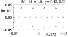
We hereafter examine the phase boundary between the nontrivial and gapless regions. Figure 6 shows the spectra in the cases of , , , and . Only the low energy region of near the real axis is shown so that we focus on chiral edge states. As discussed in Sect. 4, chiral edge states are stable only when their energies are real. In the case of , the phase boundary between the nontrivial and gapless regions is at . In panel (a) with , eigenvalues of energy at are almost equally distributed on the real axis, whereas those at deviate from the real axis, reflecting the destabilization of chiral edge states. These results are consistent with and indicate that the system changes from the nontrivial phase to the gapless phase at . Moreover, in panels (b), (c), and (d), we observe behavior similar to this; eigenvalues corresponding to chiral edge states are almost equally distributed on the real axis when and deviate from the real axis once exceeds . These results justify the phase boundary between the nontrivial and gapless regions determined in Sect. 5.
Finally, we show typical spectra in the boundary geometry to give an example of the peculiar gap closing pointed out in Sect. 5. Figure 7 shows spectra at with (a) in the nontrivial phase and (b) in the gapless phase. In the nontrivial phase, we consider that the conduction and valence bands are separated by a gap although they are linked by chiral edge states. This is because we should distinguish the chiral edge states from bulk states, as in the Hermitian limit. In the gapless phase, it should be recognized that the two bands are combined into one band by a bridge of destabilized chiral edge states. This is because the destabilized chiral edge states are bulk states.


|
7 Summary and Discussion
In two- and three-dimensional non-Hermitian topological systems, topological boundary states can be destabilized by non-Hermiticity and transformed into bulk states that bridge conduction and valence bands, resulting in a peculiar gap closing. We revised the recipe of non-Hermitian bulk–boundary correspondence [71] to take this into account, and applied it to the model of a non-Hermitian Chern insulator. [29]
In the bulk–boundary correspondence demonstrated in Sect. 5, the argument on the bulk geometry uses Eq. (92) as input. This additional input is necessary to take account of the peculiar gap closing due to the destabilization of chiral edge states. We showed that, with this input, the bulk–boundary correspondence correctly describes the boundary property specified in Fig. 3 including the destabilization of chiral edge states. Note that it is very difficult to derive the boundary property from the eigenvalue equation in the boundary geometry. This indicates that the bulk–boundary correspondence is useful in considering the boundary property of non-Hermitian topological systems.
Finally, we consider the applicability of the recipe described in Sect. 5 to a general non-Hermitian topological system in two dimensions. A phase transition of the system in the boundary geometry accompanies a gap closing, which denotes a direct touching of conduction and valence bands in a narrow sense and includes a peculiar gap closing (i.e., destabilization of boundary states that link the two bands) in a wide sense. The applicability crucially depends on low-energy states in the boundary geometry, in particular, a bulk state that is located at a touching point between the two bands. In the case of a peculiar gap closing, a bulk state should be replaced with a destabilized boundary state. This recipe is applicable if the bulk state at a touching point can be captured by the method of a separation of variables or if a non-Hermitian skin effect on it can be characterized in a quantitative manner as in Eq. (92).
Acknowledgment
This work was supported by JSPS KAKENHI Grant Number JP21K03405.
Appendix
We show that the dispersion relations given in Eqs. (73), (74), (77), and (78) are valid even when does not hold. In our system, the condition of widely holds but the condition of breaks down with increasing . When , we need to consider the boundary conditions at and on equal footing. If this is done, the eigenvalue of energy deviates from . Let us denote this deviation as and assume that is sufficiently small. We obtain the dispersion relations of chiral edge states by using the method given in Ref. \citenokamoto. Up to the first order in , the eigenvectors are modified as
| (102) | ||||
| (107) |
with
| (108) |
where , . We can ignore corrections to and , which are on the order of . Taking these into account, we construct right eigenfunctions of chiral edge states by superposing the following fundamental solutions:
| (109) | ||||
| (110) | ||||
| (111) | ||||
| (112) |
As a result, we find two eigenfunctions of with and with under the condition of
| (113) |
These eigenfunctions are given by
| (116) | ||||
| (119) |
where is a normalization constant. The left eigenfunctions corresponding to are given by
| (122) | ||||
| (125) |
The normalization constant is determined as
| (126) |
so that . In the space spanned by and , the Hamiltonian is reduced to
| (131) |
The eigenvalues of energy are obtained as
| (132) |
Equation (113) yields
| (133) |
which shows that vanishes as long as is sufficiently large and . When is ignorable, Eq. (132) is reduced to Eqs. (73) and (74).
References
- [1] D. J. Thouless, M. Kohmoto, P. Nightingale, and M. den Nijs, Phys. Rev. Lett. 49, 405 (1982).
- [2] M. Kohmoto, Ann. Phys. 160, 343 (1985).
- [3] C. L. Kane and E. J. Mele, Phys. Rev. Lett. 95, 146802 (2005).
- [4] L. Fu, C. L. Kane, and E. J. Mele, Phys. Rev. Lett. 98, 106803 (2007).
- [5] J. E. Moore and L. Balents, Phys. Rev. B 75, 121306 (2007).
- [6] R. Roy, Phys. Rev. B 79, 195322 (2009).
- [7] S. Ryu, A. P. Schnyder, A. Furusaki, and A. W. W. Ludwig, New J. Phys. 12, 065010 (2010).
- [8] L. Fu, Phys. Rev. Lett. 106, 106802 (2011).
- [9] M. Z. Hasan and C. L. Kane, Rev. Mod. Phys. 82, 3045 (2010).
- [10] X.-L. Qi and S.-C. Zhang, Rev. Mod. Phys. 83, 1057 (2011).
- [11] Y. Hatsugai, Phys. Rev. Lett. 71, 3697 (1993).
- [12] S. Ryu and Y. Hatsugai, Phys. Rev. Lett. 89, 077002 (2002).
- [13] N. Hatano and D. R. Nelson, Phys. Rev. Lett. 77, 570 (1996).
- [14] C. M. Bender and S. Boettcher, Phys. Rev. Lett. 80, 5243 (1998).
- [15] D. C. Brody, J. Phys. A 47, 035305 (2014).
- [16] Y. C. Hu and T. L. Hughes, Phys. Rev. B 84, 153101 (2011).
- [17] K. Esaki, M. Sato, K. Hasebe, and M. Kohmoto, Phys. Rev. B 84, 205128 (2011).
- [18] S. Malzard, C. Poli, and H. Schomerus, Phys. Rev. Lett. 115, 200402 (2015).
- [19] C. Yuce, Phys. Lett. A 379, 1213 (2015).
- [20] T. E. Lee, Phys. Rev. Lett. 116, 133903 (2016).
- [21] D. Leykam, K. Y. Bliokh, C. Huang, Y. D. Chong, and F. Nori, Phys. Rev. Lett. 118, 040401 (2017).
- [22] Y. Xu, S.-T. Wang, and L.-M. Duan, Phys. Rev. Lett. 118, 045701 (2017).
- [23] Y. Ashida, S. Furukawa, and M. Ueda, Nat. Commun. 8, 15791 (2017).
- [24] Y. Xiong, J. Phys. Commun. 2, 035043 (2018).
- [25] Z. Gong, Y. Ashida, K. Kawabata, K. Takasan, S. Higashikawa, and M. Ueda, Phys. Rev. X 8, 031079 (2018).
- [26] H. Shen, B. Zhen, and L. Fu, Phys. Rev. Lett. 120, 146402 (2018).
- [27] F. K. Kunst, E. Edvardsson, J. C. Budich, and E. J. Bergholtz, Phys. Rev. Lett. 121, 026808 (2018).
- [28] S. Yao and Z. Wang, Phys. Rev. Lett. 121, 086803 (2018).
- [29] S. Yao, F. Song, and Z. Wang, Phys. Rev. Lett. 121, 136802 (2018).
- [30] A. A. Zyuzin and A. Yu. Zyuzin, Phys. Rev. B 97, 041203 (2018).
- [31] S. Lieu, Phys. Rev. B 97, 045106 (2018).
- [32] V. M. Martinez Alvarez, J. E. Barrios Vargas, and L. E. F. Foa Torres, Phys. Rev. B 97, 121401 (2018).
- [33] T. Yoshida, R. Peters, and N. Kawakami, Phys. Rev. B 98, 035141 (2018).
- [34] K. Kawabata, K. Shiozaki, and M. Ueda, Phys. Rev. B 98, 165148 (2018).
- [35] C. Yin, H. Jiang, L. Li, R. Lu, and S. Chen, Phys. Rev. A 97, 052115 (2018).
- [36] K. Kawabata, S. Higashikawa, Z. Gong, Y. Ashida, and M. Ueda, Nat. Commun. 10, 297 (2019).
- [37] S. Longhi, Phys. Rev. Res. 1, 023013 (2019).
- [38] K. Yokomizo and S. Murakami, Phys. Rev. Lett. 123, 066404 (2019).
- [39] N. Okuma and M. Sato, Phys. Rev. Lett. 123, 097701 (2019).
- [40] F. Song, S. Yao, and Z. Wang, Phys. Rev. Lett. 123, 246801 (2019).
- [41] L. Herviou, J. H. Bardarson, and N. Regnault, Phys. Rev. A 99, 052118 (2019).
- [42] R. Okugawa and T. Yokoyama, Phys. Rev. B 99, 041202 (2019).
- [43] T. Yoshida, R. Peters, N. Kawakami, and Y. Hatsugai, Phys. Rev. B 99, 121101 (2019).
- [44] C. H. Lee and R. Thomale, Phys. Rev. B 99, 201103 (2019).
- [45] M. Papaj, H. Isobe, and L. Fu, Phys. Rev. B 99, 201107 (2019).
- [46] F. K. Kunst and V. Dwivedi, Phys. Rev. B 99, 245116(2019).
- [47] K.-I. Imura and Y. Takane, Phys. Rev. B 100, 165430 (2019).
- [48] L. Zhou, Phys. Rev. B 100, 184314 (2019).
- [49] K. Kawabata, K. Shiozaki, M. Ueda, and M. Sato, Phys. Rev. X 9, 041015 (2019).
- [50] L. E. F. Foa Torres, J. Phys. Mater. 3, 014002 (2019).
- [51] T. Yoshida, K. Kudo, and Y. Hatsugai, Sci. Rep. 9, 16895 (2019)
- [52] D. S. Borgnia, A. J. Kruchkov, and R.-J. Slager, Phys. Rev. Lett. 124, 056802 (2020).
- [53] Z. Yang, K. Zhang, C. Fang, and J. Hu, Phys. Rev. Lett. 125, 226402 (2020).
- [54] K. Yokomizo and S. Murakami, Phys. Rev. Res. 2, 043045 (2020).
- [55] L. Zhou, Phys. Rev. B 101, 014306 (2020).
- [56] E. Lee, H. Lee, and B.-J. Yang, Phys. Rev. B 101, 121109 (2020).
- [57] H. Wu and J.-H. An, Phys. Rev. B 102, 041119 (2020).
- [58] H. C. Wu, X. M. Yang, L. Jin, and Z. Song, Phys. Rev. B 102, 161101 (2020).
- [59] K. Mochizuki, D. Kim, N. Kawakami, and H. Obuse, Phys. Rev. A 102, 062202 (2020).
- [60] R. Koch and J. C. Budich, Eur. Phys. J. D 74, 70 (2020).
- [61] C. Yuce, Ann. Phys. (NY) 415, 168098 (2020).
- [62] F. Mostafavi, C. Yuce, O. S. Maganã-Loaiza, H. Schomerus, and H. Ramezani, Phys. Rev. Res. 2, 032057 (2020).
- [63] X.-R. Wang, C.-X. Guo, Q. Du, and S.-P. Kou, Chin. Phys. Lett. 37, 117303 (2020).
- [64] X.-L. Zhao, L.-B. Chen, L.-B. Fu, and X.-X. Yi, Ann. Phys. 532, 1900402 (2020).
- [65] Y. He and C.-C. Chien, J. Phys.: Condens. Matter 33, 085501 (2021).
- [66] K. Yokomizo and S. Murakami, Prog. Theor. Exp. Phys. 2020, 12A102 (2020).
- [67] K.-I. Imura and Y. Takane, Prog. Theor. Exp. Phys. 2020, 12A103 (2020).
- [68] H. Kondo, Y. Akagi, and H. Katsura, Prog. Theor. Exp. Phys. 2020, 12A104 (2020).
- [69] M. Kawasaki, K. Mochizuki, N. Kawakami, and H. Obuse, Prog. Theor. Exp. Phys. 2020, 12A105 (2020).
- [70] T. Yoshida, R. Peters, N. Kawakami, and Y. Hatsugai, Prog. Theor. Exp. Phys. 2020, 12A109 (2020).
- [71] Y. Takane, J. Phys. Soc. Jpn. 90, 033704 (2021).
- [72] T. Yoshida, Phys. Rev. B 103, 125145 (2021).
- [73] K. Yokomizo and S. Murakami, Phys. Rev. B 103, 165123 (2021).
- [74] R. Okugawa, R. Takahashi, and K. Yokomizo, Phys. Rev. B 103, 205205 (2021).
- [75] L. C. Xie, H. C. Wu, X. Z. Zhang, L. Jin, and Z. Song, Phys. Rev. B 104, 125406 (2021).
- [76] Y.-Q. Zhu, W. Zheng, S.-L. Zhu, and G. Palumbo, Phys. Rev. B 104, 205103 (2021).
- [77] T. Bessho and M. Sato, Phys. Rev. Lett. 127, 196404 (2021).
- [78] N. Okuma, K. Kawabata, K. Shiozaki, and M. Sato, Phys. Rev. Lett. 124, 086801 (2020).
- [79] K. Zhang, Z. Yang, and C. Fang, Phys. Rev. Lett. 125, 126402 (2020).
- [80] Y. Yi and Z. Yang, Phys. Rev. Lett. 125, 186802 (2020).
- [81] S. Longhi, Phys. Rev. B 102, 201103 (2020).
- [82] K. Kawabata, M. Sato, and K. Shiozaki, Phys. Rev. B 102, 205118 (2020).
- [83] L. Li, C.-H. Lee, S. Mu, and J. Gong, Nat. Commun. 11, 5491 (2020).
- [84] N. Okuma and M. Sato, Phys. Rev. Lett. 126, 176601(2021).
- [85] S. Longhi, Phys. Rev. B 104, 125109 (2021).
- [86] C.-X. Guo, C.-H. Liu, X.-M. Zhao, Y. Liu, and S. Chen, Phys. Rev. Lett. 127, 116801 (2021).
- [87] Y. Takane, J. Phys. Soc. Jpn. 85, 124711 (2016).
- [88] T. Sakurai and H. Sugiura, J. Comput. Appl. Math. 159, 119 (2003).
- [89] Y. Futamura, H. Tadano, T. Sakurai, JSIAM Lett. 2, 127 (2010).
- [90] P. R. Amestoy, I. S. Duff, J. Koster and J.-Y. L’Excellent, SIAM J. Matrix Anal. Appl. 23 15 (2001).
- [91] M. Okamoto, Y. Takane, and K.-I. Imura, Phys. Rev. B 89, 125425 (2014).