Phase Diagram and Crossover Phases of Topologically Ordered Graphene Zigzag Nanoribbons: Role of Localization Effects

Is the formation of a fractional charge [1, 2, 3, 4, 5, 6] a necessary and sufficient condition [7] for topologically ordered insulators [8] such as fractional quantum Hall systems [9] and interacting disordered zigzag graphene nanoribbons [10] (ZGNRs) with anyonic fractional charges? This issue is related to whether the electron localization effects destroy or enhance the topological order [11, 12, 13] and quantization of fractional charges. In a Laughlin state on a sphere (no edges present) and under weak disorder, the added electrons fractionalize and create a quasi-degenerate peak within the gap of the tunneling density of states (DOS). Electron localization [14] is expected to stabilize these fractional charges of the quasi-degenerate midgap states because these localized quasi-degenerate energy states are spatially separated from each other, as explained in [15] (if fractional charges are delocalized they overlap and become ill-defined). However, excessive disorder is considered detrimental to topological order.

In this study, we investigate similar issues with ZGNRs [16, 17, 18, 19, 20, 21, 22]. A recent study showed that weak randomness (disorder) in ZGNRs can generate $e^{-}/2$ solitonic fractional charges [23, 24, 25], which is a disorder effect closely related to the change in the disorder-free symmetry-protected topological insulator of ZGNRs to a topologically ordered [26] Mott-Anderson insulator [27, 28, 29]. These systems have a universal value for topological entanglement entropy (TEE) [11, 12] in the weak-disorder regime [30]. The shape of entanglement spectrum is also found [31] to be similar to the DOS of the edge states, as expected of topologically ordered systems [13]. In interacting disordered ZGNRs, the gap is further filled by edge states  [32, 24] with an increasing strength of the disorder potential.

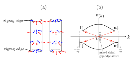
In the absence of disorder, the ground states have opposite edge site spins, but each edge is ferromagnetically polarized  [16, 17, 18, 19, 20, 21, 22]. In the presence of disorder, a spin reconstruction of the zigzag edges can occur [26]. Nonetheless, a topologically ordered ZGNR has two degenerate ground states, see Figure 1(a). Mixed chiral gap-edge states (see Figure 1(b)) play an important role in this effect. A short-range disorder potential couples two nearly chiral gap-edge states residing on opposite zigzag edges [24, 33], and mixed chiral gap-edge states with split probability densities may form to display $e^{-}/2$ fractional semion charges [34]. These states, with midgap energies, are solitonic, with half of the spectral weight originating from the conduction band and the other half from the valence band [23]. Note that a mixed chiral gap-edge state has a nonzero fractional probability at the A- and B-carbon sites. In other words, it is split into two nonlocal parts, each residing on the edges of the A or B sublattice. The formation of mixed chiral gap-edge states is a nonperturbative instanton effect [24]. (They are akin to the bonding and antibonding states of a double quantum well.) It should be noted that well-defined $e^{-}/2$ solitonic fractional charges in the weak-disorder regime are emergent particles, i.e., they have new qualitative features and appear only in sufficiently long ribbons. In a weak-disorder regime, the number of fractional charges is proportional to the length of zigzag edges.

Although weak disorder leads to formation of fractional charges, strong disorder may destroy them. Similar to fractional quantum Hall systems, the topological order of a ZGNR is not immediately destroyed upon doping because electron localization partially suppresses quantum fluctuations between quasi-degenerate mid-gap states. The system may still be an insulator with a fractional charge. However, in the presence of strong disorder or doping, zigzag edge antiferromagnetism is expected to diminish, thereby affecting the topological order. (In the doped region, a disordered anyon phase with a distorted edge spin density wave was discovered [31].) These results suggest the possibility of multiple topological phase transitions in the zigzag ribbons. What is the nature of these topological phase transitions and the physical properties of the ground states? Does the presence of a fractional charge imply a universal value of the TEE? Does the TEE become nonuniversal and vary [35] with an increase in the disorder strength or doping level?

The main results of our paper are as follows: the phase diagram of ZGNRs is found in the parameter space comprising on-site repulsion ($U$), disorder strength ($\Gamma$), and doping concentration ($\delta N/N_{s}$) ($\delta N$ and $N_{s}$ are, respectively, the number of doped electrons and the total number of sites in the ribbon). We identified a number of different phases, including those with topological order, quasi-topological order, and no order. Each of these phases is defined by the value of TEE $\beta$ and its variance. These properties of $\beta$ are related to the presence or absence of charge fractionalization and charge transfer correlations between zigzag edges. When both of these properties are present, along with correlations leading to spin-charge separation, $\beta$ is universal with small variances. In this case, we investigated the tunneling of fractional charges under an applied voltage between the zigzag edges of undoped topologically ordered zigzag ribbons and observed a possible zero-bias anomaly. The other two types of phases fall into the category of quasi-topological order. We refer to these phases as crossover phases, in which the variance of $\beta$ is significant. In one of these phases, both $e^{-}/2$ fractional charges and spin-charge separation are absent; however, the charge transfer ($\pm e^{-}/2$) correlations exist between the zigzag edges. Another phase may contain weakly stable $e^{-}/2$ fractional charges but lacks charge transfer correlations between the zigzag edges. We also investigated the ground state and zigzag edge properties of the various crossover and nontopological phases.

The following mechanisms can all give rise to fractional charges: the coupling between the valleys mediated by short-range scatterers [24] and the sublattice mixing facilitated by the alternation of the nearest neighbor hopping parameters [26]. Here we will consider the effect of short-range scatterers only. The self-consistent Hartree-Fock approximation works well for graphene systems [18, 19, 36]. The Hartree-Fock Hamiltonian of a ZGNR with length $L$ and width $W$ is

	$\displaystyle H_{\textrm{MF}}$	$\displaystyle=-t\sum_{n.n.,\sigma}c^{{\dagger}}_{i,\sigma}c_{j,\sigma}+\sum_{i,\sigma}V_{i}c_{i,\sigma}^{{\dagger}}c_{i,\sigma}$
		$\displaystyle+U\sum_{i}[n_{i,\uparrow}\langle n_{i,\downarrow}\rangle+n_{i,\downarrow}\langle n_{i,\uparrow}\rangle-\langle n_{i,\downarrow}\rangle\langle n_{i,\uparrow}\rangle]+\sum_{i}[s_{ix}\langle h_{ix}\rangle+s_{iy}\langle h_{iy}\rangle],$		(1)

where the site index is given by $i=(k,l)$ ($k$ labels sites along the ribbon direction and $l$ along the width), $c^{\dagger}_{i,\sigma}$ and $n_{i_{,}\sigma}$ represent creation and occupation operators at site $i$ with spin $\sigma=\left\{\uparrow,\downarrow\right\}$, respectively (periodic boundary conditions are used along the ribbon direction). The site spin operators are given by $s_{ix(y)}=\frac{1}{2}(c^{\dagger}_{i,\uparrow},c^{\dagger}_{i,\downarrow})\sigma^{x(y)}(c_{i,\uparrow},c_{i,\downarrow})^{T}$, where $\sigma^{x(y)}$ is the conventional Pauli matrix. The first term represents the kinetic energy with hopping parameter $t$, with $n.n$ denoting the summation over the nearest-neighbor sites. The second term represents the short-range impurities parameterized by $V_{i}$, which is randomly chosen from the energy interval $\left[-\Gamma,\Gamma\right]$. Throughout this study, the density of the impure sites is fixed at $10\%$. $U$ denotes the on-site repulsive strength. The last term in (1) represents self-consistent “magnetic fields", where $\langle h_{ix}\rangle=-2U\langle s_{ix}\rangle$ and $\langle h_{iy}\rangle=-2U\langle s_{iy}\rangle$. (These fields are present only in doped ZGNRs. In the initial stage of the Hartree-Fock iteration, the values of $\langle h_{ix}\rangle$ and $\langle h_{iy}\rangle$ can be selected from small random numbers). In the presence of these fields, the Hartree-Fock eigenstates are mixed spin states. The Hartree-Fock single-particle states $\left|k\right>$ ($k=1,2,\ldots,2N_{s}$) can be written as a linear combination of site states $\left|i,\sigma\right>$. In the language of second quantization this is equivalent to

$$a_{k}=\sum_{i,\sigma}A_{k,i,\sigma}c_{i,\sigma}.$$

(2)

These magnetic fields are rather small for the disorder strength and doping level considered in this study.

There may be several nearly degenerate Hartree-Fock ground states. We select the Hartree-Fock initial ground state such that $\langle n_{i,\sigma}\rangle$ represents a paramagnetic state with a small spin splitting. In addition, we choose small random values for $\langle h_{ix}\rangle$ and $\langle h_{iy}\rangle$ (these values do not significantly affect the final results). The Hartree-Fock matrix dimension scales with the number of carbon atoms, which is typically less than $50,000$. The Hartree-Fock eigenstates and eigenenergies are self-consistently computed, requiring approximately $20$ iterations. The TEE is computed using the disorder-averaging results from numerous disorder realizations. Here, we used GPU to speed up the solution of the Hartree-Fock matrix. The GPU calculations were computationally intensive and were performed on a supercomputer. In the presence of disorder and in the low-doping region, the obtained Hartree-Fock ground-state properties with solitons are in qualitative agreement with those of the density matrix renormalization group in the matrix product representation [31]. However, quantum fluctuations are not included in the Hartree-Fock calculation, so it may overestimate the stability of fractional charges. (In this work we do not investigate the high doping region. Obtaining density matrix renormalization group results in this region is challenging because the computation is rather time consuming, making it impossible to determine the true ground state among the nearly degenerate Hartree-Fock ground states.)

Note that the Mott gap in the absence of disorder, denoted by $\Delta$, is well-developed only when the length of the ribbon is much greater than its width $L\gg W$ (for a ribbon with $L\sim W$, its excitation spectrum is similar to that of a gapless two-dimensional graphene sheet [37]). The localization properties of ZGNRs are unusual because both localized and delocalized states can exist [24, 33]. Gap-edge states with energy $|E|\sim\Delta/2$ can have localization lengths of approximately $W$ and have significant overlap with each other.

The following simple toy model, although not realistic, is useful in understanding physics of localization [14]. Consider two localized orbital wave functions, $\phi_{1}$ and $\phi_{2}$, each having eigenenergies $\epsilon_{1}$ and $\epsilon_{2}$. Suppose these two states are coupled by an energy $I$. The Hamiltonian of the coupled system is

$$H=\begin{pmatrix}\epsilon_{1}&I\\ I&\epsilon_{2}\end{pmatrix}.$$

(3)

For the non-resonant case, where $\epsilon_{2}-\epsilon_{1}\gg I$, the perturbed eigenstates are given by

$$\psi_{1,2}\approx\phi_{1,2}+\mathcal{O}\left(\frac{I}{\epsilon_{2}-\epsilon_{1}}\right)\phi_{2,1}.$$

(4)

Thus, when the energy difference $\epsilon_{2}-\epsilon_{1}$ is greater than the hopping energy $I$, the states remain nearly unchanged, i.e., they stay localized. In the opposite resonant case, where $\epsilon_{2}-\epsilon_{1}\ll I$, the states $\phi_{1}$ and $\phi_{2}$ become strongly perturbed and transform into resonant states given by

$$\psi_{1,2}\approx\phi_{1,2}\pm\phi_{2,1}.$$

(5)

Therefore, when the energy difference is sufficiently small, the states may become delocalized, and the overlap between the localized states is significant. Symmetric and antisymmetric states of a quantum double well serve as good examples of these delocalized states.

Anderson localization plays a crucial role in the quantization of fractional charges [15]. The effects of Anderson localization can be described using self-consistent Hartree-Fock approximation [38, 39]. The first important effect of Anderson localization in undoped ribbons in the presence of on-site repulsion is that quasi-degenerate localized midgap states are spatially separated [14, 32], leading to well-defined fractional charges [15]. (In low-doped ZGNRs, added electrons fractionalize and form a narrow peak in the DOS near $E=0$ consisting of quasi-degenerate localized states  [31].) Figure 2(d) displays the probability densities of such two midgap states carrying fractional charges. These gap-edge states are mixed chiral gap-edge states [24], whose probability densities peak at the two edges and rapidly decays inside the ribbon. Note that these states do not overlap with each other. Non-interacting electrons of disordered ZGNRs also display mixed chiral gap-edge states near $E=0$. However, in the weak-disorder regime, the overlap between nearly degenerate states is small but not negligible. Thus well-defined fractional charges do not readily form in non-interacting disordered ZGNRs.

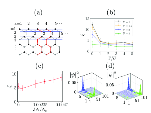
Another important effect is as follows: it affects the value of the correlation length, which is determined from the entanglement entropy of an area $A$ by computing the reduced density matrix of region $A$. The Hartree-Fock correlation function [30, 40] between $i\in A$ and $j\in A$ decays exponentially as a function of distance $x$ between $i$ and $j$

$$C(x)=C_{i\uparrow,j\uparrow}=\langle\Psi|c^{\dagger}_{i\uparrow}c_{j\uparrow}|\Psi\rangle\sim\exp\left(-\frac{|x|}{\xi}\right),$$

(6)

where $\Psi$ represents the Hartree-Fock ground state of the ZGNR, and $\xi$ represents the correlation length. By inverting the relation given in Eq.(2), we can express $c_{i\sigma}$ as a linear combination of $a_{k}$. To ensure accurate computation, the diameter of the area must be larger than the correlation length [7, 41].

The results of correlation length $\xi$ are shown in Figure 2. For disordered cases with $\Gamma\neq 0$, the correlation length is obtained by averaging over several disorder realizations. Anderson localization leads to a reduction in the correlation length when compared to disorder-free ribbons, as demonstrated in Figure 2(b). (Disorder-free ZGNRs exhibit a large correlation length for small $U$.) Therefore, compared to the non-disordered case, we can use a smaller Wilson loop [12] to calculate the TEE of disordered interacting ZGNRs. In contrast, doping results in an increased correlation length, as depicted in Figure 2(c). We stress that, in computing the correct TEE, it is important that the correlation length is small in comparison to the dimensions of the Wilson loop.

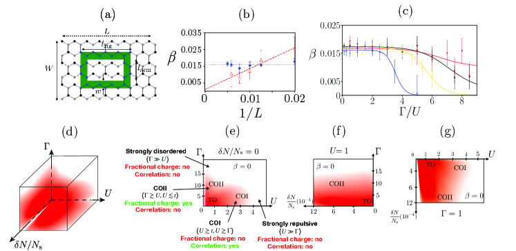
Topological order can be detected by investigating the TEE ($\beta$) [11, 12] within the Hartree-Fock approximation [30]. We begin by selecting a set of values for $(L,W,w,l_{\textrm{zig}},l_{\textrm{arm}})$, as defined in Figure 3(a), to compute $\beta$. Subsequently, we increment these quantities by the same ratio, and a new $\beta$ is computed. This process is repeated several times (see [30] for details). We employ finite-size scaling analysis to extract the TEE’s value in the limit as $L$ approaches infinity (see Figure 3(b)). We discretize the parameter space $(\Gamma,U,\delta N)$ into a three-dimensional grid, and at each grid point, we compute $\beta$ (see Figure 3(c)). The resulting three-dimensional phase diagram is depicted in Figure 3(d). We observe that $\beta$ can have three types of values: (i) A universal value in the topologically ordered phase, (ii) nonuniversal values with large variances in the crossover phases, and (iii) a zero value in the normal-disordered phase. Projections of the phase diagram, including the $U$-$\Gamma$, $\Gamma$-$\delta N$, and $U$–$\delta N$ planes, are presented in Figures 3(e)-(g).

In undoped ZGNRs, a topologically ordered phase is observed in regions $\Gamma/U\lesssim 1$ and $U\lesssim t$, see Figure 3(c). The topological phase transition into the symmetry-protected phase at $\Gamma=0$ is abrupt, consistent with findings in [30] (TEE of the symmetry-protected phase phase is zero). There are also other topological phase transitions, but they are smooth transitions with crossover regions. Note that the system is not topologically ordered at $U=0$: our Hartree-Fock results show that fractional charges overlap with each other and charge-transfer correlations are absent. Figures 3(e)-(g) reveal the presence of crossover regimes lying beyond the topologically ordered phase with an increase in the disorder, doping, and interaction strength. The phase boundaries between topologically ordered and normal phases are “blurred,” indicating the presence of crossover phases (comprising two types, crossover phase I and crossover phase II). The numerical results of the TEE are shown in Figure 3(c). The error bars in this figure include not only random fluctuations caused by disorder but also the uncertainties arising from the extrapolation process of the finite scaling analysis. As $\Gamma/U$ increases, $\beta$ decreases (indicated by the red line in Figure 3(b)). The value of the TEE thus changes across a crossover phase. Within this phase, $\beta$ exhibits a large variance, but the average values are not zero, which implies that the topological order is not completely destroyed. In this regime, the TEE becomes nonuniversal and decays.

One can use a different but equivalent procedure to determine the phase diagram. We have verified that a similar phase diagram can be obtained by analyzing the presence of fractional charges and nonlocal correlations between the opposite zigzag edges. For each grid point $(\Gamma,U,\delta N)$ in the parameter space, we find the ground state and investigate whether the gap-edge states display fractional charges and whether nonlocal correlations exist between the opposite zigzag edges. By utilizing this method, we have successfully recovered the phase diagram depicted in Figure 3(d).

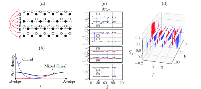
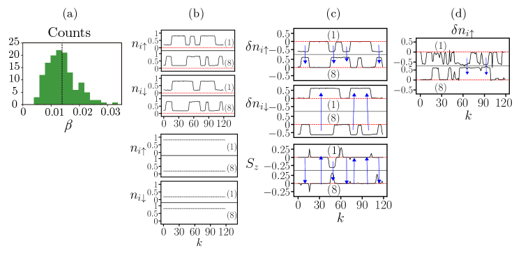
We elucidate the nature of non-local correlations in topologically ordered ZGNRs. Figure 4(a) presents a ZGNR consisting of 8 carbon lines labeled $l=1,2,\ldots,8$. In each pair of carbons lines $(1,8)$, $(2,7)$, $(3,6)$, and $(4,5)$, an increase/decrease in the occupation number of one line is correlated with a decrease/increase in that of the other line (as illustrated by lines 1 and 8 in Figure 4(c)). This correlation is not limited to the zigzag edges but extends to other carbon lines inside the ribbon, away from the edges. The corresponding site spins of the ribbon are shown in Figure 4 (d). These non-local correlations are attributed to mixed chiral gap-edge states (which can decay relatively slowly from the zigzag edges, unlike the fractional edge states), as schematically represented in Figure 4(b). Changes in the occupation numbers $\delta n_{i,\uparrow}$ and $\delta n_{i,\downarrow}$ of an edge often coincide at nearly the same values as $k$, which labels the site position along the ribbon direction. This effect can lead to $n_{i,\uparrow}\approx n_{i,\downarrow}$ of the occupation numbers in the presence of disorder, resulting in $s_{i}\approx 0$, i.e., the appearance of spin-charge separation around a site on one of the edges [26].

The following points should be noted as well. The results in Figure 3(c) show that the variance of $\beta$ decreases as we approach the singular limit of $\Gamma/U\rightarrow 0$. (Additional numerical results confirm this conclusion.) This result is consistent with the previous finding that fractional charge of a midgap state becomes accurate in the weak disorder regime and in the thermodynamic limit (as discussed in [31]). In the opposite limit of $\Gamma/U\gg 1$, the value of the TEE becomes non-universal and decreases with increasing $U$ (as shown in Figure 3(c)). In addition, the functional dependence of DOS on $E$ in the universal region is given by an exponentially suppressed function, a linear function [26], or something in between. The actual shape of the DOS is determined by the competition between the strength of disorder and the on-site repulsion [29]. For instance, the DOS is linear for $(U,\Gamma,\delta N)=(2t,0.5t,0),$ but it is exponentially suppressed in the weak disorder limit.

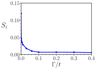
Disorder is a singular perturbation[26] and it significantly impacts the properties of zigzag ribbons, particularly noticeable when measuring the average site spin value along a zigzag edge. Our analysis reveals a dramatic alteration in this value concerning the disorder strength $\Gamma$: a singularity in the slope emerges, as depicted in Fig. 5.

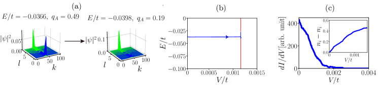
Here we also investigate the tunneling of fractional charge between two zigzag edges [43, 44]. We initiate the investigation by considering a gap-edge state that displays fractional charges in the undoped case, as illustrated in Figure 6(a). We then examine how the probability density of this state evolves as the voltage V between the zigzag edges increases. The transformation of the probability density during the tunneling event is plotted in Figure 6(a). One peak tunnels across the width of the ZGNR and merges with the other peak located at the opposite edge to form an integer charge. Since tunneling of fractional charges occurs within a narrow range of applied voltage $V$, as shown in Figure 6(b), our results suggest the potential existence of a zero-bias anomaly in the differential conductance, see Figure 6(c).

We will provide a comprehensive description of the characteristics of undoped ZGNRs in the crossover I phase, with $U\gtrsim t$ and $U\gtrsim\Gamma$, where the dominant energy is the on-site repulsion $U$. The topologically ordered phase gradually changes into the crossover I phase as $U$ increases, as illustrated in Figure 3(e). In this phase, $\beta$ is nonzero, but its variance is significant, as shown in Figure 7(a). The crossover I phase exhibits the following notable properties: (i) The disorder-induced change in the edge occupation numbers $\delta n_{i,\uparrow}=1/2$ for one type of spin $\sigma$ is entirely transferred to the opposite edge, i.e., the zigzag edges are correlated in a nontrivial manner, as shown in Figure 7(c) for a specific case of $\Gamma/U=0.17$. However, the site positions $k$ on the opposite zigzag edges, where changes in $\delta n_{i,\uparrow}$ and $\delta n_{i,\downarrow}$ occur do not coincide. (This is in contrast to the topologically ordered phase where these positions exhibit correlations at nearly identical $k$ values.) We believe that these edge transfer correlations between zigzag edges modify the ground state entanglement pattern and yield a nonzero fluctuating TEE. The edge charge transfer correlations become weaker when the disorder is stronger (see Figure 7(d) for $\Gamma/t=4$), leading to a smaller value of $\beta$ (see Figure 3(c)). (ii) Although the zigzag edge changes are fractional, $\delta n_{i,\uparrow}=1/2$, as shown in Figures 7(b) and (c)), the A- and B-probability densities of the mixed chiral gap-edge states responsible for this feature overlap, see Figure 4(b). Consequently, fractional charges are ill-defined in this phase. (iii) The presence of spin-charge separation necessitates that charge transfers for both spin types occur at the same positions $k$. However, these effects are not observed in the crossover I phase. It is essential to emphasize that the condition $S_{z}=\frac{1}{2}(n_{i,\uparrow}-n_{i,\downarrow})=0$ at site $i$ is not sufficient for spin-charge separation. To fulfill the conditions, well-defined fractional charges must exist.

For undoped ZGNRs, another crossover phase emerges when $\Gamma\gg U$ but $U/t\lesssim 1$. We call this phase crossover II where the disorder strength $\Gamma$ is the dominant energy. As $\Gamma$ increases, the topologically ordered phase undergoes a gradual transition into the crossover phase II, as depicted in Figure 3(e). Concurrently, the gap is progressively filled with states, as illustrated in the upper graph of Figure 8(a). Similar to the crossover I phase (Figure 7(a)), $\beta$ is finite with a significant variance. However, in this phase, there are no charge-transfer correlations between the zigzag edges, as evident from the lower graph in Figure 8(a). Some fractional charges may exist, as shown in Figure 8(b), but they are expected to be subject to greater quantum fluctuations.

This observation aligns with the following obtained results: (i) Some changes in the edge occupation number are $\delta n_{i,\sigma}\approx\pm 1/2$. (ii) There are gap-edge states with $q_{A}\approx 1/2$. (Here $q_{A}=\sum_{i\in A}|\psi_{i\sigma}(E)|^{2}$, where $\psi_{i\sigma}(E)$ is the Hartree-Fock eigenstate with energy $E$, see [26]. The probability densities are summed over all sites of the A sublattice.) However, although the mean value of $q_{A}$ is $1/2$, its variance in the energy interval $[E-\delta E,E+\delta E]$ is large because $q_{A}$ varies substantially within this interval, as shown in Figure 8(a). Despite this, a fractional charge of a state in the interval $[E-\delta E,E+\delta E]$ near $E=0$ does not overlap significantly with the probability densities of other fractional and non-fractional states in the same energy interval, provided that $\delta E$ is small (for $U\sim t$ and $\Gamma\sim t$, this happens when $\delta E\sim 0.01t$). (However, in the absence of on-site repulsion, multiple states with the same value of $\delta E$ overlap.) We posit that the interplay between localization and on-site repulsion accounts for these non-overlapping states, as previously discussed at the outset of Sec.3. Nevertheless, the impact of quantum fluctuations [15] must not be disregarded, as significant overlap with states in the adjacent energy intervals may occur. (The Hartree-Fock calculation, which ignores quantum fluctuations, may thus overestimate the stability of fractional charges.)

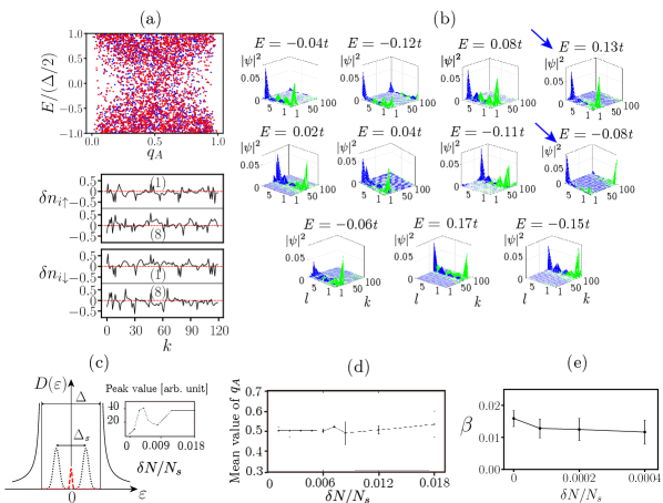
So far, our investigation has primarily focused on the undoped case. Upon doping, the disorder-free ZGNRs exhibit edge spin density waves, with the opposite edges still being antiferromagnetically coupled. This is in contrast to the edge ferromagnetism observed in undoped ribbons. If disorder is added to a doped ZGNR, the spin waves become distorted [31]: There is a topological phase transition from modulated ferromagnetic edges at zero doping to distorted spin-wave edges at finite doping. Our results indicated that, under substantial doping, this phase is also a crossover phase II. The dependence of the mean value of $q_{A}$ of the states within the midgap peak on the number of doped electrons is illustrated in Figure 8(d) (the DOS shows a sharp peak at the midgap energy as seen in Figure 8(c)). At a low doping concentration, the disorder-averaged value of $q_{A}$ of the midgap peak is close to $0.5$, and the midgap states display well-defined fractional charges with small variance, as discussed below Fig. 2 (note that the width of the midgap peak is $\delta E\sim 0.005t$). As the doping concentration increases further, $q_{A}$ significantly deviates from 0.5, and simultaneously, the DOS midgap peak starts to decrease [31]. These findings imply that even though fractional charges can still be observed, their number decreases with an increase in doping. The gradual change in $q_{A}$ as a function of $\delta N/N_{\textrm{s}}$ indicates that the transition from the phase of the distorted ferromagnetic edge to the phase of the distorted edge spin-wave is not sharp. Figure 8(e) shows how $\beta$ decreased with an increase in $\delta N/N_{\textrm{s}}$. For a large $\delta N/N_{\textrm{s}}$, it is computationally demanding to calculate $\beta$ due to the anticipated longer correlation length, as observed in Figure 2(c).

Let us discuss the strongly disordered phase within the region $\Gamma/U\gg 1$ as indicated in Figure 3(e). The topological order is destroyed once the disorder strength reaches a sufficiently high level, for example, $\beta=0$ at $(U,\Gamma,\delta N)=(t,15t,0)$. Within this region, both edge charge-transfer correlations and charge fractionalization are not well-defined, implying a TEE of zero. In Figure 9(a), site occupation numbers in weak ($\Gamma=0.03t$) and strong ($\Gamma=15t$) disorder regimes are shown side by side to highlight the difference, where the ones in strong disorder regime highly fluctuate from site to site. Moreover, edge magnetization is zero almost everywhere (see Figure 9(b)). The occupation numbers display sharp values of $n_{i,\sigma}=1$ at some sites, a feature also observed in the density matrix renormalization group calculations of disordered ribbons, as reported in [31].

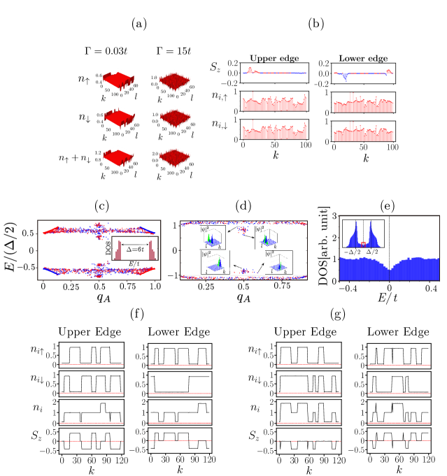
Another phase emerges in the form of the strongly repulsive phase ($U\gg t$) where fractional charges and zigzag edge correlations become non-existent. As depicted in Figure 3(e), $\beta\approx 0$ characterizes this phase. The $q_{A}$–$E$ diagram in Figure 9(c) highlights the nonperturbative nature of disorder in this regime: the values $q_{A}$ are scattered across the entire spectrum between $0$ and $1$ as $\Gamma\rightarrow 0$, whereas they are restricted to the four solid lines at $\Gamma=0$. Also, the $(E,q_{A})$ distribution indicates that in this strongly repulsive regime, even with the presence of disorder, a large energy gap persists. There are no states with $q_{A}\approx 1/2$ in the vicinity the midgap energy, as illustrated in Figure 9(c). The A- and B-components of the wave function of the states with $q_{A}\approx 1/2$ near the gap edges $\pm\Delta/2$ overlap, as revealed in Figure 9(d). For a stronger disorder (equivalently a larger value of $\Gamma$), the gap becomes increasingly filled with states, leading to a DOS finite at $E=0$, as shown in Figure 9(e).

The main physics characterizing this phase becomes apparent by investigating the zigzag edge structure: the occupation numbers take on values of $n_{i,\sigma}=1$ or $0$ so charge transfers are one ($\delta n_{i,\sigma}=\pm 1$) in the strongly repulsive phase (the total site occupation number of each site is $n_{i}\approx 2$, $1$, or $0$ despite a strong on-site repulsion $U$). It is important to note that no transfer of fractional charges was observed between zigzag edges. This absence of charge transfer is attributed to the absence of mixed chiral gap-edge states. Additionally, it is worth mentioning that the edge magnetization displays sharp domain walls, as evidenced in Figures 9(f)-(g).

We computed the phase diagram of zigzag graphene nanoribbons as a function of the on-site repulsion $U$, doping $\delta N$, and disorder strength $\Gamma$. Our analysis identified the universal, crossover, strongly disordered, and strongly repulsive phases. Each phase of the phase diagram was defined by the TEE value and its variance. We also investigated how the values of the TEE are related to the following physical properties: the presence of charge fractionalization and the edge charge transfer correlations between the opposite zigzag edges. When both of these properties are present, along with correlations leading to spin-charge separation, $\beta$ was universal. If only one of these properties was present, $\beta$ was nonuniversal and its variance was significant. However, when both properties were entirely absent, $\beta$ was approximately zero. These results suggest that non-local correlations in zigzag ribbons give rise to non-zero TEE values. Furthermore, our investigation identified a strongly repulsive phase with zero TEE in large on-site repulsion and weak disorder limits. Its ground state contains abrupt kinks in zigzag edge magnetizations without charge fractionalization, which is a consequence of the singular perturbative nature of the disorder potential. An additional phase with zero TEE was identified, corresponding to the strongly disordered regime $\Gamma\gg U$. In this phase, the edge site occupation numbers fluctuate highly from site to site, and antiferromagnetic coupling between the two edges is nearly destroyed. Each phase of the phase diagram presents a distinct zigzag-edge structure.

We also conducted an investigation into the effect of the interplay between localization and on-site repulsion on the charge quantization. In low-doped and/or weakly disordered ZGNRs, this interplay contributes to the spatial separation of quasi-degenerate gap-edge states, and protects the charge fractionalization against quantum fluctuations. Even in the presence of moderately strong disorder, charge fractionalization is not completely eradicated.

Reference [42] showed that, in the absence of disorder, there can be several different antiferromagnetic and ferromagnetic phase changes as width and doping concentration increase. In our work, we have investigated ribbons with widths smaller than $\sim 10$ nm and doping concentrations less than $\sim 0.003$. We focused on the low doping region of disordered ribbons because our investigation shows that topological order is stable only in that regime. In this low doping region, each edge develops a spin density wave [31]. However, the average site spin values of the opposite edges are still being antiferromagnetically coupled.

We briefly discuss some experimental implications. Investigating the tunneling of fractional charges between the zigzag edges of undoped, topologically ordered zigzag ribbons under an applied voltage could be an interesting avenue, similar to experiments performed on fractional quantum Hall edges [43, 44]. Such an effect may lead to a zero-bias anomaly. Additionally, observing the presence of nonlocal charge transfers between the zigzag edges of the crossover phase I would be of interest. This can be investigated by measuring correlations between the edge site occupation numbers using a scanning tunneling microscope [45]. In the crossover phase II, fractional $e^{-}/2$ edge charges are present; however, unusual transport and magnetic susceptibility properties are not expected due to the absence of spin-charge separation. (In contrast, the topologically ordered phase is expected to display unusual transport and magnetic susceptibility because of spin-charge separation [46, 26].) Similarly, using scanning tunneling microscopy can help to validate the predicted edge occupation numbers in the strongly repulsive and strongly disordered phases.

S.R.E.Y. was supported by the Basic Science Research Program of the National Research Foundation of Korea (NRF), funded by the Ministry of Science and ICT (MSIT) NRF-2021R1F1A1047759. Two other grants are also acknowledged: BK21 FOUR (Fostering Outstanding Universities for Research) and KISTI Supercomputing Center with supercomputing resources including technical support KSC-2022-CRE-0345.

References

- [1] Jon Magne Leinaas and Jan Myrheim. “On the theory of identical particles”. Nuovo Cimento B 37, 1–23 (1977).
- [2] Frank Wilczek. “Quantum mechanics of fractional-spin particles”. Phys. Rev. Lett. 49, 957–959 (1982).
- [3] Daniel Arovas, J. R. Schrieffer, and Frank Wilczek. “Fractional statistics and the quantum hall effect”. Phys. Rev. Lett. 53, 722–723 (1984).
- [4] J. Nakamura, S. Liang, G. C. Gardner, and M. J. Manfra. “Direct observation of anyonic braiding statistics”. Nature Physics 16, 931–936 (2020).
- [5] H. Bartolomei, M. Kumar, R. Bisognin, A. Marguerite, J.-M. Berroir, E. Bocquillon, B. Plaçais, A. Cavanna, Q. Dong, U. Gennser, Y. Jin, and G. Fève. “Fractional statistics in anyon collisions”. Science 368, 173–177 (2020).
- [6] Steven M Girvin and Kun Yang. “Modern condensed matter physics”. Cambridge University Press. Cambridge (2019).
- [7] Jianis K Pachos. “Introduction to topological quantum computation”. Cambridge University Press. Cambridge (2012).
- [8] Xiao-Gang Wen. “Colloquium: Zoo of quantum-topological phases of matter”. Rev. Mod. Phys. 89, 041004 (2017).
- [9] R. B. Laughlin. “Anomalous quantum hall effect: An incompressible quantum fluid with fractionally charged excitations”. Phys. Rev. Lett. 50, 1395–1398 (1983).
- [10] S.-R. Eric Yang. “Topologically ordered zigzag nanoribbon”. World Scientific, Singapore. (2023).
- [11] Alexei Kitaev and John Preskill. “Topological entanglement entropy”. Phys. Rev. Lett. 96, 110404 (2006).
- [12] Michael Levin and Xiao-Gang Wen. “Detecting topological order in a ground state wave function”. Phys. Rev. Lett. 96, 110405 (2006).
- [13] Hui Li and F. D. M. Haldane. “Entanglement spectrum as a generalization of entanglement entropy: Identification of topological order in non-abelian fractional quantum hall effect states”. Phys. Rev. Lett. 101, 010504 (2008).
- [14] B. Altshuler. “Inductory anderson localization”. In Advanced Workshop on Anderson Localization, Nonlinearity and Turbulence: a Cross-Fertilization. International Centre for Theoretical Physics (2010).
- [15] Steven M Girvin. “The quantum hall effect: novel excitations and broken symmetries”. In Aspects topologiques de la physique en basse dimension. Topological aspects of low dimensional systems. Pages 53–175. Springer (1999).
- [16] Mitsutaka Fujita, Katsunori Wakabayashi, Kyoko Nakada, and Koichi Kusakabe. “Peculiar localized state at zigzag graphite edge”. J. Phys. Soc. Jpn. 65, 1920–1923 (1996).
- [17] L. Brey and H. A. Fertig. “Electronic states of graphene nanoribbons studied with the dirac equation”. Phys. Rev. B 73, 235411 (2006).
- [18] Li Yang, Cheol-Hwan Park, Young-Woo Son, Marvin L. Cohen, and Steven G. Louie. “Quasiparticle energies and band gaps in graphene nanoribbons”. Phys. Rev. Lett. 99, 186801 (2007).
- [19] L. Pisani, J. A. Chan, B. Montanari, and N. M. Harrison. “Electronic structure and magnetic properties of graphitic ribbons”. Phys. Rev. B 75, 064418 (2007).
- [20] Pascal Ruffieux, Shiyong Wang, Bo Yang, Carlos Sánchez-Sánchez, Jia Liu, Thomas Dienel, Leopold Talirz, Prashant Shinde, Carlo A Pignedoli, Daniele Passerone, et al. “On-surface synthesis of graphene nanoribbons with zigzag edge topology”. Nature 531, 489–492 (2016).
- [21] Marek Kolmer, Ann-Kristin Steiner, Irena Izydorczyk, Wonhee Ko, Mads Engelund, Marek Szymonski, An-Ping Li, and Konstantin Amsharov. “Rational synthesis of atomically precise graphene nanoribbons directly on metal oxide surfaces”. Science 369, 571–575 (2020).
- [22] Luis Brey, Pierre Seneor, and Antonio Tejeda, editors. “Graphene nanoribbons”. 2053-2563. IOP Publishing. (2019).
- [23] A. J. Heeger, S. Kivelson, J. R. Schrieffer, and W. P. Su. “Solitons in conducting polymers”. Rev. Mod. Phys. 60, 781–850 (1988).
- [24] Y. H. Jeong, S.-R. Eric Yang, and Min-Chul Cha. “Soliton fractional charge of disordered graphene nanoribbon”. Journal of Physics: Condensed Matter 31, 265601 (2019).
- [25] S.-R. Eric Yang. “Soliton fractional charges in graphene nanoribbon and polyacetylene: similarities and differences”. Nanomaterials 9, 885 (2019).
- [26] S.-R. Eric Yang, Min-Chul Cha, Hye Jeong Lee, and Young Heon Kim. “Topologically ordered zigzag nanoribbon: fractional edge charge, spin-charge separation, and ground-state degeneracy”. Phys. Rev. Research 2, 033109 (2020).
- [27] Vladimir Dobrosavljevic, Nandini Trivedi, and James M. Valles, Jr. “Conductor-Insulator Quantum Phase Transitions”. Oxford University Press. (2012).
- [28] D. Belitz and T. R. Kirkpatrick. “The anderson-mott transition”. Rev. Mod. Phys. 66, 261–380 (1994).
- [29] Krzysztof Byczuk, Walter Hofstetter, and Dieter Vollhardt. “Competition between anderson localization and antiferromagnetism in correlated lattice fermion systems with disorder”. Phys. Rev. Lett. 102, 146403 (2009).
- [30] Young Heon Kim, Hye Jeong Lee, and S.-R. Eric Yang. “Topological entanglement entropy of interacting disordered zigzag graphene ribbons”. Phys. Rev. B 103, 115151 (2021).
- [31] Young Heon Kim, Hye Jeong Lee, Hyun-Yong Lee, and S.-R. Eric Yang. “New disordered anyon phase of doped graphene zigzag nanoribbon”. Scientific Reports 12, 14551 (2022).
- [32] Al L Éfros and Boris I Shklovskii. “Coulomb gap and low temperature conductivity of disordered systems”. Journal of Physics C: Solid State Physics 8, L49–L51 (1975).
- [33] Leandro R. F. Lima, Felipe A. Pinheiro, Rodrigo B. Capaz, Caio H. Lewenkopf, and Eduardo R. Mucciolo. “Effects of disorder range and electronic energy on the perfect transmission in graphene nanoribbons”. Phys. Rev. B 86, 205111 (2012).
- [34] G. S. Canright, S. M. Girvin, and A. Brass. “Superconductive pairing of fermions and semions in two dimensions”. Phys. Rev. Lett. 63, 2295–2298 (1989).
- [35] Ching-Yu Huang and Feng-Li Lin. “Topological order and degenerate singular value spectrum in two-dimensional dimerized quantum heisenberg model”. Phys. Rev. B 84, 125110 (2011).
- [36] T. Stauber, P. Parida, M. Trushin, M. V. Ulybyshev, D. L. Boyda, and J. Schliemann. “Interacting electrons in graphene: Fermi velocity renormalization and optical response”. Phys. Rev. Lett. 118, 266801 (2017).
- [37] A. H. Castro Neto, F. Guinea, N. M. R. Peres, K. S. Novoselov, and A. K. Geim. “The electronic properties of graphene”. Rev. Mod. Phys. 81, 109–162 (2009).
- [38] S.-R. Eric Yang, A. H. MacDonald, and Bodo Huckestein. “Interactions, localization, and the integer quantum hall effect”. Phys. Rev. Lett. 74, 3229–3232 (1995).
- [39] S.-R. Eric Yang and A. H. MacDonald. “Coulomb gaps in a strong magnetic field”. Phys. Rev. Lett. 70, 4110–4113 (1993).
- [40] Ingo Peschel. “Calculation of reduced density matrices from correlation functions”. Journal of Physics A: Mathematical and General 36, L205 (2003).
- [41] H-C. Jiang, Z. Wang, and L. Balents. “Identifying topological order by entanglement entropy”. Nature Phys 8, 902–905 (2012).
- [42] W.-C. Chen, Y. Zhou, S.-L. Yu, W.-G. Yin, and C.-D. Gong. “Width-Tuned Magnetic Order Oscillation on Zigzag Edges of Honeycomb Nanoribbons”. Nano Lett., 17(7), 4400–4404 (2017).
- [43] W Kang, HL Stormer, LN Pfeiffer, KW Baldwin, and KW West. “Tunnelling between the edges of two lateral quantum hall systems”. Nature 403, 59–61 (2000).
- [44] I. Yang, W. Kang, K. W. Baldwin, L. N. Pfeiffer, and K. W. West. “Cascade of quantum phase transitions in tunnel-coupled edge states”. Phys. Rev. Lett. 92, 056802 (2004).
- [45] Eva Y Andrei, Guohong Li, and Xu Du. “Electronic properties of graphene: a perspective from scanning tunneling microscopy and magnetotransport”. Reports on Progress in Physics 75, 056501 (2012).
- [46] T.-C. Chung, F. Moraes, J. D. Flood, and A. J. Heeger. “Solitons at high density in trans-: Collective transport by mobile, spinless charged solitons”. Phys. Rev. B 29, 2341–2343 (1984).
Acknowledgements