This paper was converted on www.awesomepapers.org from LaTeX by an anonymous user.
Want to know more? Visit the Converter page.

Pfaffian solution for dark-dark soliton to the coupled complex modified Korteweg-de Vries equation

Chenxi Li Chenxi Li
School of Mathematics and Statistics, Xi’an Jiaotong University, Xi’an, Shaanxi 710049, P.R. China
[email protected]
Xiaochuan Liu Xiaochuan Liu
School of Mathematics and Statistics, Xi’an Jiaotong University, Xi’an, Shaanxi 710049, P.R. China
[email protected]
 and  Bao-Feng Feng Corresponding author: Bao-Feng Feng
School of Mathematics and Statistical Sciences, The University of Texas Rio Grande Valley, Edinburg, TX 78539, USA
[email protected]
Abstract.

In this paper, we study coupled complex modified Korteweg-de Vries (ccmKdV) equation by combining the Hirota’s method and the Kadomtsev-Petviashvili (KP) reduction method. First, we show that the bilinear form of the ccmKdV equation under nonzero boundary condition is linked to the discrete BKP hierarchy through Miwa transformation. Based on this finding, we construct the dark-dark soliton solution in the pfaffian form. The dynamical behaviors for one- and two-soliton are analyzed and illustrated.

Key words and phrases: dark soliton solution; pfaffian solution; Kadomtsev-Petviashvili (KP) reduction method; Miwa transformation.

1. Introduction

Higher-order nonlinear Schrödinger (HONLS) equation

iqt+α1qxx+α2|q|2q+i(β1qxxx+β2|q|2qx+β3q(|q|2)x)=0,\mathrm{i}q_{t}+\alpha_{1}q_{xx}+\alpha_{2}|q|^{2}q+\mathrm{i}(\beta_{1}q_{xxx}+\beta_{2}|q|^{2}q_{x}+\beta_{3}q(|q|^{2})_{x})=0\,, (1.1)

was first developed by Kodama and Hasegawa in the nonlinear optics [2]. The parameter α2>0\alpha_{2}>0 denotes the Kerr effect-induced self-phase modulation(SPM) , while α1\alpha_{1} governs the group velocity dispersion (GVD): α1>0\alpha_{1}>0 is focusing case [3], whereas for α1<0\alpha_{1}<0 is defocusing case [4]. Here, β1\beta_{1}, β2\beta_{2}, and β3\beta_{3} determine three fundamental higher-order effects: third-order dispersion, self-steepening, and stimulated Raman scattering, respectively [5]. In some special cases, Eq. (1.1) becomes integrable when specific constraints on parameters βi\beta_{i} are imposed. For instance, several well-known integrable models have emerged: (i) the Kaup-Newell equation [6] (β1=0,β2:β3=1:1\beta_{1}=0,\beta_{2}:\beta_{3}=1:1), (ii) the Chen-Lee-Liu equation [7] (β1=β3=0\beta_{1}=\beta_{3}=0), (iii) the Hirota equation [8] (β1:β2:β3=1:6:0\beta_{1}:\beta_{2}:\beta_{3}=1:6:0 ), (iv) the Sasa-Satsuma (SS) equation [9] (β1:β2:β3=1:6:3\beta_{1}:\beta_{2}:\beta_{3}=1:6:3).

Due to the polarization of propagation pulses, the coupled models of the HONLS are important in practical applications [10, 11, 12]. In other words, a coupled NLS equation with extra dispersion and nonlinear terms is more practical in nonlinear optics. As discussed in [13], there are several two-component generalizations of the HONLS equation which are integrable . These integrable models include

  1. (1)

    The coupled Hirota equation [14]

    u1,t=u1,xxx3c(|u1|2+|u2|2)u1,x3cu1(u1u1,x+u2u2,x),\displaystyle u_{1,t}=u_{1,xxx}-3c(|u_{1}|^{2}+|u_{2}|^{2})u_{1,x}-3cu_{1}(u^{*}_{1}u_{1,x}+u^{*}_{2}u_{2,x}), (1.2)
    u2,t=u2,xxx3c(|u1|2+|u2|2)u2,x3cu2(u1u1,x+u2u2,x).\displaystyle u_{2,t}=u_{2,xxx}-3c(|u_{1}|^{2}+|u_{2}|^{2})u_{2,x}-3cu_{2}(u^{*}_{1}u_{1,x}+u^{*}_{2}u_{2,x}). (1.3)
  2. (2)

    The coupled Sasa-Satsuma (CSS) equation [15]

    u1,t=u1,xxx3c(|u1|2+|u2|2)u1,x3cu1(|u1|2+|u2|2)x,\displaystyle u_{1,t}=u_{1,xxx}-3c(|u_{1}|^{2}+|u_{2}|^{2})u_{1,x}-3cu_{1}(|u_{1}|^{2}+|u_{2}|^{2})_{x}, (1.4)
    u2,t=u2,xxx3c(|u1|2+|u2|2)u2,x3cu2(|u1|2+|u2|2)x.\displaystyle u_{2,t}=u_{2,xxx}-3c(|u_{1}|^{2}+|u_{2}|^{2})u_{2,x}-3cu_{2}(|u_{1}|^{2}+|u_{2}|^{2})_{x}. (1.5)
  3. (3)

    The coupled complex modified Korteweg-de Vries (ccmKdV) equation [16]

    u1,t=u1,xxx3c(|u1|2+|u2|2)u1,x,\displaystyle u_{1,t}=u_{1,xxx}-3c(|u_{1}|^{2}+|u_{2}|^{2})u_{1,x}, (1.6)
    u2,t=u2,xxx3c(|u1|2+|u2|2)u2,x.\displaystyle u_{2,t}=u_{2,xxx}-3c(|u_{1}|^{2}+|u_{2}|^{2})u_{2,x}\,. (1.7)

There are much more studies for the coupled Hirota equation than for the CSS and the ccmKdV equations probably due to the reason that it is the simplest equation among three integrable cases (see, for example, Refs. [17, 18, 19, 20, 21]). In the original paper by Tasgal et al. [14], the bright soliton was obtained by using the inverse scattering transformation. Bright, dark and bright-dark soliton solutions were constructed by various researchers [17, 22, 23, 24]. Recently, rogue wave solutions of the coupled Hirota equation were developed in [20, 25, 21, 26].

The soliton solutions of the CSS equation were mainly constructed by the Darboux transformation. In [27], the authors constructed the single- and double-hump solutions under the zero boundary condition, which were expressed as Wronskian determinants. Bright multi-soliton solutions were derived and the energy transfer mechanism was revealed in [28, 29]. The rational solutions in localized conditions under non-zero boundaries were established in [30], in which the authors revealed the dark-antidark soliton, W-shape solution, Mexican hat, and anti-Mexican hat solutions. In [31], both bright and dark solitons were studied, with single and bright hump solutions found on a vanishing background and an anti-dark soliton solution found on a non-vanishing background. In [32], the dark-bright soliton and semirational rogue wave solutions were derived via the Darboux-dressing method.

On the other hand, the Riemann-Hilbert problem to the CSS equation was formulated and studied in [33, 34, 35, 36], in which the soliton solutions and their asymptotic properties are reported. Most recently, Zhang et al. derived the bilinear form of the CSS equation and constructed various soliton solutions such as the dark, breather, and rogue wave solutions by the Kadomtsev-Petviashvili (KP) reduction method [37, 38]. Moreover, the bright-bright, dark-dark, and bright-dark soliton solutions are obtained by applying the KP reduction method [39].

In spite of the fact that the ccmKdV equation (1.6)–(1.7) is a straightforward generalization of the complex mKdV equation

ut=uxxx3c|u|2ux,u_{t}=u_{xxx}-3c|u|^{2}u_{x}, (1.8)

the associated study related to the ccmKdV equation is much less compared with the coupled Hirota and CSS equations. The pfaffian form of the general bright soliton solution to the multi-component mKdV equation was given by Iwao and Hirota [40]. Tsuchida studied the coupled mKdV equation using the inverse scattering transformation [41]. By using Hirota’s bilinear method, one- and two-bright soliton and breather solutions [42], as well as the first-order rogue wave solution, were constructed in [43].

A 4×44\times 4 Lax pair of the ccmKdV equation (1.6)–(1.7) was given by Tsuchida [41] as Φx=UΦ\Phi_{x}=U\Phi, Φt=VΦ\Phi_{t}=V\Phi with

U=iλ(IOOI)+(OQRO),\displaystyle U=\mathrm{i}\lambda\begin{pmatrix}-I&O\\ O&I\end{pmatrix}+\begin{pmatrix}O&Q\\ R&O\end{pmatrix},
V=\displaystyle V= iλ3(4IOO4I)+λ2(O4Q4RO)+iλ(2QR2Qx2Rx2RQ)\displaystyle\mathrm{i}\lambda^{3}\begin{pmatrix}-4I&O\\ O&4I\end{pmatrix}+\lambda^{2}\begin{pmatrix}O&4Q\\ 4R&O\end{pmatrix}+\mathrm{i}\lambda\begin{pmatrix}-2QR&2Q_{x}\\ -2R_{x}&2RQ\end{pmatrix}
+(QxRQRxQxx+2QRQRxx+2RQRRxQRQx),\displaystyle+\begin{pmatrix}Q_{x}R-QR_{x}&-Q_{xx}+2QRQ\\ -R_{xx}+2RQR&R_{x}Q-RQ_{x}\end{pmatrix},
Q=c2(u1u2u2u1),R=c2(u1u2u2u1),\displaystyle Q=\sqrt{\dfrac{c}{2}}\begin{pmatrix}u_{1}&u_{2}\\ -u^{*}_{2}&u^{*}_{1}\end{pmatrix},\ \ R=\sqrt{\dfrac{c}{2}}\begin{pmatrix}u^{*}_{1}&-u_{2}\\ u^{*}_{2}&u_{1}\end{pmatrix},

where λ\lambda is the spectral parameter that is independent of time. u1u_{1} and u2u_{2} are complex-valued functions. II is the 2×22\times 2 identity matrix. OO is the 2×22\times 2 zero matrix. It is noticed that system (1.6)–(1.7) also admits a 6×66\times 6 Lax pair in [44].

Due to the pfaffian structure of the soliton solution to the ccmKdV equation, its multi-dark soliton solution under nonzero boundary condition remains an unsolved problem, which is the motivation of the present paper. The remainder of the paper is organized as follows: In Section 2, the main result for the dark-dark soliton solution in pfaffian is presented by bilinearizing the ccmKdV equation (1.6)–(1.7). The proof of the main result is given in Section 3. The dynamics analysis for one- and two-soliton solutions is constructed in Section 4.

2. Bilinearization and dark soliton solutions under nonzero boundary condition

In this section, we will give the bilinear form of the coupled complex mKdV equation (1.6)–(1.7) under a nonzero boundary condition. To this end, we assume the following transformations

u1=ρ1g1fei(α1xω1t),u2=ρ2g2fei(α2xω2t),u_{1}=\rho_{1}\frac{g_{1}}{f}e^{\mathrm{i}\left(\alpha_{1}x-\omega_{1}t\right)},\quad u_{2}=\rho_{2}\frac{g_{2}}{f}e^{\mathrm{i}\left(\alpha_{2}x-\omega_{2}t\right)}, (2.1)

where ff is a real-valued function, g1,g2g_{1},g_{2} are complex-valued functions, and ρi\rho_{i} and αi\alpha_{i} are real parameters, ωi=αi3+3cαi(ρ12+ρ22),i=1,2.\omega_{i}=\alpha^{3}_{i}+3c\alpha_{i}(\rho_{1}^{2}+\rho_{2}^{2}),i=1,2.

By substituting (2.1) into (1.6), we obtain

f2(Dx3Dt+3iα1Dx23α12Dx3c(ρ12+ρ22)Dx)g1f\displaystyle f^{2}(D^{3}_{x}-D_{t}+3\mathrm{i}\alpha_{1}D^{2}_{x}-3\alpha^{2}_{1}D_{x}-3c(\rho_{1}^{2}+\rho_{2}^{2})D_{x})\,g_{1}\cdot f
3(Dxg1f)(Dx2ff+c(ρ12|g1|2+ρ22|g2|2)c(ρ12+ρ22)f2)\displaystyle-3(D_{x}g_{1}\cdot f)(D^{2}_{x}f\cdot f+c(\rho_{1}^{2}|g_{1}|^{2}+\rho_{2}^{2}|g_{2}|^{2})-c(\rho_{1}^{2}+\rho_{2}^{2})f^{2}) (2.2)
3iα1g1f(Dx2ff+c(ρ12|g1|2+ρ22|g2|2)c(ρ12+ρ22)f2)=0,\displaystyle-3\mathrm{i}\alpha_{1}g_{1}f\,(D^{2}_{x}f\cdot f+c(\rho_{1}^{2}|g_{1}|^{2}+\rho_{2}^{2}|g_{2}|^{2})-c(\rho_{1}^{2}+\rho_{2}^{2})f^{2})=0\,,

where DD is the Hirota’s bilinear operator [45] defined by

DxmDtnfg=(xx)m(tt)n[f(x,t)g(x,t)]|x=x,t=t.\displaystyle D_{x}^{m}D_{t}^{n}f\cdot g=\left.\left(\frac{\partial}{\partial x}-\frac{\partial}{\partial{x^{\prime}}}\right)^{m}\left(\frac{\partial}{\partial t}-\frac{\partial}{\partial{t^{\prime}}}\right)^{n}[f(x,t)g(x^{\prime},t^{\prime})]\right|_{x^{\prime}=x,t^{\prime}=t}.

If we require

Dx2ff+c(ρ12|g1|2+ρ22|g2|2)=c(ρ12+ρ22)f2,\displaystyle D^{2}_{x}f\cdot f+c(\rho_{1}^{2}|g_{1}|^{2}+\rho_{2}^{2}|g_{2}|^{2})=c(\rho_{1}^{2}+\rho_{2}^{2})f^{2}, (2.3)

we obtained

(Dx3Dt+3iα1Dx23(α12+c(ρ12+ρ22))Dx)g1f=0.(D_{x}^{3}-D_{t}+3\mathrm{i}\alpha_{1}D_{x}^{2}-3(\alpha_{1}^{2}+c(\rho_{1}^{2}+\rho_{2}^{2}))D_{x})g_{1}\cdot f=0.

Similarly, the bilinear form for (1.7) can also get. Thus, the resulting bilinear equations are

(Dx3Dt+3iα1Dx23(α12+c(ρ12+ρ22))Dx)g1f=0,\displaystyle(D_{x}^{3}-D_{t}+3\mathrm{i}\alpha_{1}D_{x}^{2}-3(\alpha_{1}^{2}+c(\rho_{1}^{2}+\rho_{2}^{2}))D_{x})\,g_{1}\cdot f=0\,, (2.4a)
(Dx3Dt+3iα2Dx23(α22+c(ρ12+ρ22))Dx)g2f=0,\displaystyle(D_{x}^{3}-D_{t}+3\mathrm{i}\alpha_{2}D_{x}^{2}-3(\alpha_{2}^{2}+c(\rho_{1}^{2}+\rho_{2}^{2}))D_{x})\,g_{2}\cdot f=0\,, (2.4b)
(Dx2c(ρ12+ρ22))ff=c(ρ12|g1|2+ρ22|g2|2).\displaystyle(D^{2}_{x}-c(\rho_{1}^{2}+\rho_{2}^{2}))\,f\cdot f=-c(\rho_{1}^{2}|g_{1}|^{2}+\rho_{2}^{2}|g_{2}|^{2})\,. (2.4c)

If we introduce the following transformation,

x~=x3c(ρ12+ρ22)t,t~=t,\displaystyle\tilde{x}=x-3c(\rho_{1}^{2}+\rho_{2}^{2})t,\ \ \tilde{t}=t, (2.5)

the above equations can be rewritten as

(Dx3Dt+3iα1Dx23α12Dx)g~1f~=0,\displaystyle(D_{x}^{3}-D_{t}+3\mathrm{i}\alpha_{1}D_{x}^{2}-3\alpha_{1}^{2}D_{x})\,\tilde{g}_{1}\cdot\tilde{f}=0\,, (2.6a)
(Dx3Dt+3iα2Dx23α22Dx)g~2f~=0,\displaystyle(D_{x}^{3}-D_{t}+3\mathrm{i}\alpha_{2}D_{x}^{2}-3\alpha_{2}^{2}D_{x})\,\tilde{g}_{2}\cdot\tilde{f}=0\,, (2.6b)
(Dx2c(ρ12+ρ22))f~f~=c(ρ12|g~1|2+ρ22|g~2|2),\displaystyle(D^{2}_{x}-c(\rho_{1}^{2}+\rho_{2}^{2}))\,\tilde{f}\cdot\tilde{f}=-c(\rho_{1}^{2}|\tilde{g}_{1}|^{2}+\rho_{2}^{2}|\tilde{g}_{2}|^{2})\,, (2.6c)

where f~=f~(x~,t~),gi~=gi~(x~,t~),i=1,2.\tilde{f}=\tilde{f}(\tilde{x},\tilde{t}),\tilde{g_{i}}=\tilde{g_{i}}(\tilde{x},\tilde{t}),i=1,2. Therefore, the ccmKdV equation (1.6)–(1.7) can be transformed into the bilinear equations (2.6a)–(2.6c) via the transformations (2.1) and (2.5).

We convert the solution of system (1.6)–(1.7) to the solution of (2.6a)–(2.6c). In what follows, we construct solutions satisfying (2.6a)–(2.6c) for c=1c=1, and they are expressed in pfaffian.

Theorem 2.1.

The dark-dark soliton solution of the ccmKdV equation (1.6)–(1.7) satisfies

u1=ρ1g1fei(α1x(α13+3cα1(ρ12+ρ22))t),u2=ρ2g2fei(α2x(α23+3cα2(ρ12+ρ22))t),u_{1}=\rho_{1}\frac{g_{1}}{f}e^{\mathrm{i}\left(\alpha_{1}x-(\alpha^{3}_{1}+3c\alpha_{1}(\rho_{1}^{2}+\rho_{2}^{2}))t\right)},\ \ u_{2}=\rho_{2}\frac{g_{2}}{f}e^{\mathrm{i}\left(\alpha_{2}x-(\alpha^{3}_{2}+3c\alpha_{2}(\rho_{1}^{2}+\rho_{2}^{2}))t\right)}, (2.7)

where

f=τ0,0(x3c(ρ12+ρ22)t,t),g1=τ1,0(x3c(ρ12+ρ22)t,t),g2=τ0,1(x3c(ρ12+ρ22)t,t),f=\tau_{0,0}\left(x-3c(\rho_{1}^{2}+\rho_{2}^{2})t,t\right),\ \ g_{1}=\tau_{1,0}\left(x-3c(\rho_{1}^{2}+\rho_{2}^{2})t,t\right),\ \ g_{2}=\tau_{0,1}\left(x-3c(\rho_{1}^{2}+\rho_{2}^{2})t,t\right),

The pfaffian τk1,k2\tau_{k_{1},k_{2}} given by

τk1,k2=(1,2,,2N)\tau_{k_{1},k_{2}}=(1,2,\cdots,2N) (2.8)

with

(i,j)=δ2N+1i,j+pipjpi+pj(d0,i)(d0,j),i<j\displaystyle(i,j)=\delta_{2N+1-i,j}+\frac{p_{i}-p_{j}}{p_{i}+p_{j}}(d_{0},i)(d_{0},j),\ \ i<j (2.9)
(d0,i)=ν=12(piiανpi+iαν)kνexpξi,ξi=pix+pi3t+ξi0,\displaystyle(d_{0},i)=\prod_{\nu=1}^{2}\left(\frac{p_{i}-\mathrm{i}\alpha_{\nu}}{p_{i}+\mathrm{i}\alpha_{\nu}}\right)^{k_{\nu}}\exp\xi_{i},\ \ \xi_{i}=p_{i}x+p_{i}^{3}t+\xi_{i0}, (2.10)

the parameters pip_{i} and ξi0\xi_{i0} are complex constants and satisfying the reduction condition

2α12ρ12(pi2+α12)(pi2+α12)+2α22ρ22(pi2+α22)(pi2+α22)=1,\displaystyle\frac{2{\alpha_{1}}^{2}{\rho_{1}}^{2}}{(p^{2}_{i}+\alpha^{2}_{1})({p^{*}_{i}}^{2}+\alpha^{2}_{1})}+\frac{2{\alpha_{2}}^{2}{\rho_{2}}^{2}}{(p^{2}_{i}+\alpha^{2}_{2})({p^{*}_{i}}^{2}+\alpha^{2}_{2})}=1, (2.11)

where p2N+1i=pi,p_{2N+1-i}=p^{*}_{i}, and ξ2N+1i=ξi+iπ/2\xi_{2N+1-i}=\xi^{*}_{i}+\mathrm{i}\pi/2 for 1iN.1\leq i\leq N.

3. Derivation of the dark soliton solution

In this section, we will derive multi-dark soliton solution to the ccmKdV equation (1.6)–(1.7) which satisfy three bilinear equations (2.6a)–(2.6c). We start with a lemma, which can be deduced from the discrete BKP hierarchy.

Lemma 3.1.

The pfaffian

τk1,k2=(1,2,,2N),\displaystyle\tau_{k_{1},k_{2}}=(1,2,\cdots,2N)\,, (3.1)

with its elements defined by

(i,j)=cij+pipjpi+pj(d0,i)(d0,j),(d0,i)=ν=12(pi+aνpiaν)kνexpξi,\displaystyle(i,j)=c_{ij}+\frac{p_{i}-p_{j}}{p_{i}+p_{j}}(d_{0},i)(d_{0},j),\ \ (d_{0},i)=\prod_{\nu=1}^{2}\left(\frac{p_{i}+a_{\nu}}{p_{i}-a_{\nu}}\right)^{k_{\nu}}\ \exp\xi_{i}\,, (3.2)

where ξi=pix1+pi3x3+ξi0\xi_{i}=p_{i}x_{1}+p_{i}^{3}x_{3}+\xi_{i0} and cij=cjic_{ij}=-c_{ji}, pip_{i}, ξi0\xi_{i0}, a1a_{1}, a2a_{2} are constants, satisfies the bilinear equations

(Dx13Dx33a1Dx12+3a12Dx1)τk1+1,k2τk1,k2=0,\displaystyle\left(D_{x_{1}}^{3}-D_{x_{3}}-3a_{1}D_{x_{1}}^{2}+3a_{1}^{2}D_{x_{1}}\right)\tau_{k_{1}+1,k_{2}}\cdot\tau_{k_{1},k_{2}}=0\,, (3.3)
(Dx13Dx33a2Dx12+3a22Dx1)τk1,k2+1τk1,k2=0.\displaystyle\left(D_{x_{1}}^{3}-D_{x_{3}}-3a_{2}D_{x_{1}}^{2}+3a_{2}^{2}D_{x_{1}}\right)\tau_{k_{1},k_{2}+1}\cdot\tau_{k_{1},k_{2}}=0\,. (3.4)
Proof.

The discrete BKP equation was proposed by Miwa [46]. The pfaffian solution to the discrete BKP equation was given by Tsujimoto and Hirota [47]. Similarly to the discrete KP equation, the discrete BKP equation can be extended to the discrete BKP hierarchy in the sense that the same bilinear equation holds from an arbitrary triple (ki,kj,km)(k_{i},k_{j},k_{m}) with discrete parameters (ai,aj,am)(a_{i},a_{j},a_{m}). Here we choose a pafffian with four discrete variables

τ(k1,k2,k3,k4)=(1,2,,2N),\tau(k_{1},k_{2},k_{3},k_{4})=(1,2,\cdots,2N)\,, (3.5)

with

(i,j)=cij+pipjpi+pjϕi(k1,k2,k3,k4)ϕj(k1,k2,k3,k4),\displaystyle(i,j)=c_{ij}+\frac{p_{i}-p_{j}}{p_{i}+p_{j}}\phi_{i}(k_{1},k_{2},k_{3},k_{4})\phi_{j}(k_{1},k_{2},k_{3},k_{4})\,, (3.6)
cij=cji,ϕi(k1,k2,k3,k4)=ν=14(1aν1pi1+aν1pi)kν.\displaystyle c_{ij}=-c_{ji},\ \ \phi_{i}(k_{1},k_{2},k_{3},k_{4})=\prod_{\nu=1}^{4}\left(\frac{1-a^{-1}_{\nu}p_{i}}{1+a^{-1}_{\nu}p_{i}}\right)^{-k_{\nu}}\,. (3.7)

If we pick up a triple (k1,k3,k4k_{1},k_{3},k_{4}) then we have

(a3a4)(a1+a3)(a1+a4)τ1τ34+(a4a1)(a3+a4)(a3+a1)τ3τ41\displaystyle(a_{3}-a_{4})(a_{1}+a_{3})(a_{1}+a_{4})\tau_{1}{\tau}_{34}+(a_{4}-a_{1})(a_{3}+a_{4})(a_{3}+a_{1})\tau_{3}{\tau}_{41}
+(a1a3)(a4+a1)(a4+a3)τ4τ13+(a1a3)(a3a4)(a4a1)ττ134=0.\displaystyle+(a_{1}-a_{3})(a_{4}+a_{1})(a_{4}+a_{3})\tau_{4}{\tau}_{13}+(a_{1}-a_{3})(a_{3}-a_{4})(a_{4}-a_{1})\tau{\tau}_{134}=0\,. (3.8)

Here each subscript ii denotes a forward shift in the corresponding discrete variable nin_{i}, for example, τi=τ(ki+1,kj,km)\tau_{i}=\tau(k_{i}+1,k_{j},k_{m}), τij=τ(ki+1,kj+1,km)\tau_{ij}=\tau(k_{i}+1,k_{j}+1,k_{m}). Notice that

((1al1pi)(1al1pj)(1+al1pi)(1+al1pj))kl\displaystyle\left(\frac{(1-a^{-1}_{l}p_{i})(1-a^{-1}_{l}p_{j})}{(1+a^{-1}_{l}p_{i})(1+a^{-1}_{l}p_{j})}\right)^{-k_{l}} =\displaystyle= exp(klln((1al1pi)(1al1pj)(1+al1pi)(1+al1pj)))\displaystyle\exp\left(-k_{l}\ln\left(\frac{(1-a^{-1}_{l}p_{i})(1-a^{-1}_{l}p_{j})}{(1+a^{-1}_{l}p_{i})(1+a^{-1}_{l}p_{j})}\right)\right)
=\displaystyle= exp(2al1kl(pi+pj)+23al3kl(pi3+pj3)+),\displaystyle\exp\left(2a^{-1}_{l}k_{l}(p_{i}+p_{j})+\frac{2}{3}a_{l}^{-3}k_{l}(p_{i}^{3}+p_{j}^{3})+\cdots\right)\,,

we can define the so-called Miwa transformation

x1=2i=34kiai1,x3=23i=34kiai3,,x2μ1=22μ1i=34kiai2μ+1.x_{1}=2\sum^{4}_{i=3}k_{i}a^{-1}_{i},\ x_{3}=\frac{2}{3}\sum^{4}_{i=3}k_{i}a_{i}^{-3},\ \cdots,\ x_{2\mu-1}=\frac{2}{2\mu-1}\sum^{4}_{i=3}k_{i}a_{i}^{-2\mu+1}.

Furthermore, we can define the elementary Schur polynomial

exp(tnxn)=pn(x)tn,\exp\left(\sum t^{n}x_{n}\right)=\sum p_{n}(\vec{x})t^{n}\,,

where

x=(x1,x2,,xn),\vec{x}=(x_{1},x_{2},\cdots,x_{n})\,,
p0=1,p1(x)=x1,p2=x2+12x12,,p3=x3+x1x2+16x13,p_{0}=1,\ p_{1}(x)=x_{1},\ p_{2}=x_{2}+\frac{1}{2}x_{1}^{2},\cdots,p_{3}=x_{3}+x_{1}x_{2}+\frac{1}{6}x_{1}^{3},
pn=k1+2k2++nkn=nx1k1x2k2xnknk1!k2!kn!.p_{n}=\sum_{k_{1}+2k_{2}+\cdots+nk_{n}=n}\frac{x_{1}^{k_{1}}x_{2}^{k_{2}}\cdots x_{n}^{k_{n}}}{k_{1}!k_{2}!\cdots k_{n}!}\,.

Then, the discrete BKP equation (3) can be converted into

((a3a4)(a1+a3)(a1+a4)a3La4MpL(D~)pM(D~)\displaystyle((a_{3}-a_{4})(a_{1}+a_{3})(a_{1}+a_{4})\sum a_{3}^{-L}a_{4}^{-M}p_{L}(-\mathaccent 869{D})p_{M}(-\mathaccent 869{D})
+(a4a1)(a3+a4)(a3+a1)a3La4MpL(D~)pM(D~)\displaystyle+(a_{4}-a_{1})(a_{3}+a_{4})(a_{3}+a_{1})\sum a_{3}^{-L}a_{4}^{-M}p_{L}(-\mathaccent 869{D})p_{M}(\mathaccent 869{D})
+(a1a3)(a4+a1)(a4+a3)a3La4MpL(D~)pM(D~)\displaystyle+(a_{1}-a_{3})(a_{4}+a_{1})(a_{4}+a_{3})\sum a_{3}^{-L}a_{4}^{-M}p_{L}(\mathaccent 869{D})p_{M}(-\mathaccent 869{D})
+(a1a3)(a3a4)(a4a1)a3La4MpL(D~)pM(D~))τk1+1,k2τk1,k2=0.\displaystyle+(a_{1}-a_{3})(a_{3}-a_{4})(a_{4}-a_{1})\sum a_{3}^{-L}a_{4}^{-M}p_{L}(\mathaccent 869{D})p_{M}(\mathaccent 869{D}))\tau_{k_{1}+1,k_{2}}\cdot\tau_{k_{1},k_{2}}=0\,.

Here D~=(Dx1,0,13Dx3,0,)\mathaccent 869{D}=(D_{x_{1}},0,\frac{1}{3}D_{x_{3}},0,\cdots). At the order of a31a4a^{-1}_{3}a_{4}, we have

(4p3(D~)4p1(D~)p2(D~)+4a1p12(D~)4a12p1(D~))τk1+1,k2τk1,k2=0,\displaystyle(4p_{3}(\mathaccent 869{D})-4p_{1}(\mathaccent 869{D})p_{2}(\mathaccent 869{D})+4a_{1}p^{2}_{1}(\mathaccent 869{D})-4a^{2}_{1}p_{1}(\mathaccent 869{D}))\tau_{k_{1}+1,k_{2}}\cdot\tau_{k_{1},k_{2}}=0\,,

which is nothing but the bilinear equation (3.3). Similarly, starting from

(a3a4)(a2+a3)(a2+a4)τ2τ34+(a4a2)(a3+a4)(a3+a2)τ3τ42\displaystyle(a_{3}-a_{4})(a_{2}+a_{3})(a_{2}+a_{4})\tau_{2}{\tau}_{34}+(a_{4}-a_{2})(a_{3}+a_{4})(a_{3}+a_{2})\tau_{3}{\tau}_{42}
+(a2a3)(a4+a2)(a4+a3)τ4τ23+(a2a3)(a3a4)(a4a2)ττ234=0,\displaystyle+(a_{2}-a_{3})(a_{4}+a_{2})(a_{4}+a_{3})\tau_{4}{\tau}_{23}+(a_{2}-a_{3})(a_{3}-a_{4})(a_{4}-a_{2})\tau{\tau}_{234}=0\,, (3.9)

by picking up a triple of (k2,k3,k4k_{2},k_{3},k_{4}), we can approve (3.4). ∎

Remark: The same bilinear equations (2.6a) and (2.6b) were approved by the identities of pfaffian in [48]. The lemma given below is approved in Appendix by pfaffian identities.

Lemma 3.2.

If cij=δ2N+1i,jc_{ij}=\delta_{2N+1-i,j}, 1i<j2N1\leq i<j\leq 2N, then under the condition

2a12ρ12(pj2a12)(p2N+1j2a12)+2a22ρ22(pj2a22)(p2N+1j2a22)=1,\displaystyle\frac{2{a_{1}}^{2}{\rho_{1}}^{2}}{(p^{2}_{j}-a^{2}_{1})(p^{2}_{2N+1-j}-a^{2}_{1})}+\frac{2{a_{2}}^{2}{\rho_{2}}^{2}}{(p^{2}_{j}-a^{2}_{2})(p^{2}_{2N+1-j}-a^{2}_{2})}=-1\,, (3.10)

the pfaffian (3.1) satisfies the following bilinear equation

(Dx2(ρ12+ρ22))τk1,k2τk1,k2=(ρ12τk1+1,k2τk11,k2+ρ22τk1,k2+1τk1,k21).\displaystyle(D^{2}_{x}-(\rho_{1}^{2}+\rho_{2}^{2}))\tau_{k_{1},k_{2}}\cdot\tau_{k_{1},k_{2}}=-(\rho_{1}^{2}\tau_{k_{1}+1,k_{2}}\tau_{k_{1}-1,k_{2}}+\rho_{2}^{2}\tau_{k_{1},k_{2}+1}\tau_{k_{1},k_{2}-1})\,.{} (3.11)

Proof of the Lemma is given in Appendix. We note that the equations in the BKP hierarchy exhibit a structure akin to that presented in (2.6a)-(2.6c), albeit with supplementary conditions. This insight prompts us to explore the complex conjugate reduction.

Lemma 3.3.

If we choose a1=iα1a_{1}=-\mathrm{i}\alpha_{1}, a2=iα2a_{2}=-\mathrm{i}\alpha_{2} to be purely imaginary numbers, cij=δ2N+1i,jc_{ij}=\delta_{2N+1-i,j} for 1i<j2N1\leq i<j\leq 2N, and p2N+1i=pi,p_{2N+1-i}=p^{*}_{i}, ξ2N+1i=ξi+iπ/2\xi_{2N+1-i}=\xi^{*}_{i}+\mathrm{i}\pi/2 for 1iN1\leq i\leq N in pfaffian (3.1), it it shown that

τ¯k1,k2=τk1,k2.\displaystyle\overline{\tau}_{k_{1},k_{2}}=\tau_{-k_{1},-k_{2}}. (3.12)
Proof.

Using the above conditions, we find

(d0,i)¯\displaystyle\overline{(d_{0},i)} =iν=12(p2N+1iiανp2N+1i+iαν)kνeξ2N+1i=i(d0,2N+1i)k1,k2, 1i2N\displaystyle=-\mathrm{i}\prod_{\nu=1}^{2}\left(\frac{p_{2N+1-i}-\mathrm{i}\alpha_{\nu}}{p_{2N+1-i}+\mathrm{i}\alpha_{\nu}}\right)^{-k_{\nu}}e^{\xi_{2N+1-i}}=-\mathrm{i}(d_{0},2N+1-i)_{-k_{1},-k_{2}}\,,\ \ \ \ \ \ 1\leq i\leq 2N
(i,j)¯\displaystyle\overline{(i,j)} =δ2N+1i,jp2N+1ip2N+1jp2N+1i+p2N+1j(d0,2N+1i)k1,k2(d0,2N+1j)k1,k2\displaystyle=-\delta_{2N+1-i,j}-\dfrac{p_{2N+1-i}-p_{2N+1-j}}{p_{2N+1-i}+p_{2N+1-j}}(d_{0},2N+1-i)_{-k_{1},-k_{2}}(d_{0},2N+1-j)_{-k_{1},-k_{2}}
=(2N+1i,2N+1j)k1,k2\displaystyle=-(2N+1-i,2N+1-j)_{-k_{1},-k_{2}}
=(2N+1j,2N+1i)k1,k2, 1i<j2N\displaystyle=(2N+1-j,2N+1-i)_{-k_{1},-k_{2}}\,,\ \ \ \ 1\leq i<j\leq 2N

Therefore,

τ¯k1,k2\displaystyle\overline{\tau}_{k_{1},k_{2}} =((2N+1j,2N+1i)k1,k2)1i<j2N=(1,2,,2N)k1,k2=τk1,k2.\displaystyle=((2N+1-j,2N+1-i)_{-k_{1},-k_{2}})_{1\leq i<j\leq 2N}=(1,2,\ldots,2N)_{-k_{1},-k_{2}}=\tau_{-k_{1},-k_{2}}.

Finally, we define

f~=τ00,g~1=τ1,0,g~2=τ0,1,\displaystyle\tilde{f}=\tau_{00},\quad\tilde{g}_{1}=\tau_{1,0},\quad\tilde{g}_{2}=\tau_{0,1}, (3.13)

then we have

f~=f~,g~1=τ1,0,g~2=τ0,1.\displaystyle\tilde{f}=\tilde{f}^{*},\quad\tilde{{g}}^{*}_{1}=\tau_{-1,0},\quad\tilde{{g}}^{*}_{2}=\tau_{0,-1}. (3.14)

Combining Lemma 3.1– Lemma 3.3, the pfaffian solutions to the bilinear equations (2.6a)-(2.6c) are derived.

4. Dynamics of one- and two-soliton solutions

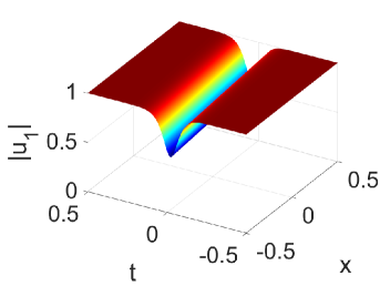
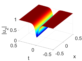
Theorem 2.1 gives the dark-dark soliton solution (2.7) of the ccmKdV equation (1.6)-(1.7). By taking N=1N=1, we obtain the one-soliton solution in which f,g1,g2f,g_{1},g_{2} are

f\displaystyle f =1+ip1p1p1+p1exp(ξ1+ξ1),\displaystyle=1+\mathrm{i}\;\dfrac{p_{1}-p^{*}_{1}}{p_{1}+p^{*}_{1}}\exp{(\xi_{1}+\xi^{*}_{1})}\,,
g1\displaystyle g_{1} =1+ip1p1p1+p1(p1iα1p1+iα1)(p1iα1p1+iα1)exp(ξ1+ξ1),\displaystyle=1+\mathrm{i}\;\dfrac{p_{1}-p^{*}_{1}}{p_{1}+p^{*}_{1}}\left(\dfrac{p_{1}-\mathrm{i}\alpha_{1}}{p_{1}+\mathrm{i}\alpha_{1}}\right)\left(\dfrac{p^{*}_{1}-\mathrm{i}\alpha_{1}}{p^{*}_{1}+\mathrm{i}\alpha_{1}}\right)\exp{(\xi_{1}+\xi^{*}_{1})}\,,
g2\displaystyle g_{2} =1+ip1p1p1+p1(p1iα2p1+iα2)(p1iα2p1+iα2)exp(ξ1+ξ1),\displaystyle=1+\mathrm{i}\;\dfrac{p_{1}-p^{*}_{1}}{p_{1}+p^{*}_{1}}\left(\dfrac{p_{1}-\mathrm{i}\alpha_{2}}{p_{1}+\mathrm{i}\alpha_{2}}\right)\left(\dfrac{p^{*}_{1}-\mathrm{i}\alpha_{2}}{p^{*}_{1}+\mathrm{i}\alpha_{2}}\right)\exp{(\xi_{1}+\xi^{*}_{1})}\,,

where the ξ1=p1(x3(ρ12+ρ22)t)+p13t+ξ10,\xi_{1}=p_{1}(x-3(\rho^{2}_{1}+\rho^{2}_{2})t)+p^{3}_{1}t+\xi_{10}\,, and p1p_{1} satisfy the reduction relation. The one-soliton solution is expressed as
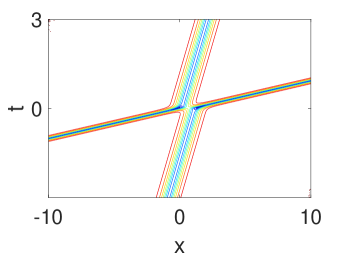
u1=ρ1exp(iθ1)\displaystyle u_{1}=\rho_{1}\exp(\mathrm{i}\theta_{1}) [12(1+(p1iα1p1+iα1)(p1iα1p1+iα1))\displaystyle\left[\dfrac{1}{2}\left(1+\left(\dfrac{p_{1}-\mathrm{i}\alpha_{1}}{p_{1}+\mathrm{i}\alpha_{1}}\right)\left(\dfrac{p^{*}_{1}-\mathrm{i}\alpha_{1}}{p^{*}_{1}+\mathrm{i}\alpha_{1}}\right)\right)\right.
12(1(p1iα1p1+iα1)(p1iα1p1+iα1))tanh(Re(ξ1)+12log(iIm(p1)Re(p1)))],\displaystyle\left.-\dfrac{1}{2}\left(1-\left(\dfrac{p_{1}-\mathrm{i}\alpha_{1}}{p_{1}+\mathrm{i}\alpha_{1}}\right)\left(\dfrac{p^{*}_{1}-\mathrm{i}\alpha_{1}}{p^{*}_{1}+\mathrm{i}\alpha_{1}}\right)\right)\tanh\left(\mathrm{Re}(\xi_{1})+\dfrac{1}{2}\mathrm{log}(\mathrm{i}\dfrac{\mathrm{Im}(p_{1})}{\mathrm{Re}(p_{1})})\right)\right],
u2=ρ2exp(iθ2)\displaystyle u_{2}=\rho_{2}\exp(\mathrm{i}\theta_{2}) [12(1+(p1iα2p1+iα2)(p1iα2p1+iα2))\displaystyle\left[\dfrac{1}{2}\left(1+\left(\dfrac{p_{1}-\mathrm{i}\alpha_{2}}{p_{1}+\mathrm{i}\alpha_{2}}\right)\left(\dfrac{p^{*}_{1}-\mathrm{i}\alpha_{2}}{p^{*}_{1}+\mathrm{i}\alpha_{2}}\right)\right)\right.
12(1(p1iα2p1+iα2)(p1iα2p1+iα2))tanh(Re(ξ1)+12log(iIm(p1)Re(p1)))],\displaystyle\left.-\dfrac{1}{2}\left(1-\left(\dfrac{p_{1}-\mathrm{i}\alpha_{2}}{p_{1}+\mathrm{i}\alpha_{2}}\right)\left(\dfrac{p^{*}_{1}-\mathrm{i}\alpha_{2}}{p^{*}_{1}+\mathrm{i}\alpha_{2}}\right)\right)\tanh\left(\mathrm{Re}(\xi_{1})+\dfrac{1}{2}\mathrm{log}(\mathrm{i}\dfrac{\mathrm{Im}(p_{1})}{\mathrm{Re}(p_{1})})\right)\right]\,,

where the θi=αix(αi3+3αi(ρ12+ρ22))t,\theta_{i}=\alpha_{i}x-(\alpha^{3}_{i}+3\alpha_{i}(\rho^{2}_{1}+\rho^{2}_{2}))t, i=1,2.i=1,2. We can plot the one dark soliton solutions, see Fig. 1.

Refer to caption
Refer to caption
Figure 1. One dark soliton solutions to the ccmKdV equation (1.6)–(1.7) with parameters p1p_{1} = 0.88 + i, ρ1=1,α1=2\rho 1=1,\,\alpha 1=2, ρ2=1,α2=1.\rho 2=1,\,\alpha 2=1. (a) and (b) are profiles of |u1||u_{1}| and |u2||u_{2}|, respectively.

Taking N=2N=2, we get the two-soliton solution

f\displaystyle f =1+C1exp(ξ1+ξ1)+C2exp(ξ2+ξ2)+C1C2Mexp(ξ1+ξ1+ξ2+ξ2),\displaystyle=1+C_{1}\exp{(\xi_{1}+\xi^{*}_{1})}+C_{2}\exp{(\xi_{2}+\xi^{*}_{2})}+C_{1}C_{2}\mathrm{M}\exp{(\xi_{1}+\xi^{*}_{1}+\xi_{2}+\xi^{*}_{2})}\,,
g1\displaystyle g_{1} =1+C1A1exp(ξ1+ξ1)+C2A2exp(ξ2+ξ2)+C1C2A1A2Mexp(ξ1+ξ1+ξ2+ξ2),\displaystyle=1+C_{1}A_{1}\exp{(\xi_{1}+\xi^{*}_{1})}+C_{2}A_{2}\exp{(\xi_{2}+\xi^{*}_{2})}+C_{1}C_{2}A_{1}A_{2}\mathrm{M}\exp{(\xi_{1}+\xi^{*}_{1}+\xi_{2}+\xi^{*}_{2})}\,,
g2\displaystyle g_{2} =1+C1B1exp(ξ1+ξ1)+C2B2exp(ξ2+ξ2)+C1C2B1B2Mexp(ξ1+ξ1+ξ2+ξ2),\displaystyle=1+C_{1}B_{1}\exp{(\xi_{1}+\xi^{*}_{1})}+C_{2}B_{2}\exp{(\xi_{2}+\xi^{*}_{2})}+C_{1}C_{2}B_{1}B_{2}\mathrm{M}\exp{(\xi_{1}+\xi^{*}_{1}+\xi_{2}+\xi^{*}_{2})}\,,

and

Cj=ipjpjpj+pj\displaystyle C_{j}=\mathrm{i}\,\dfrac{p_{j}-p^{*}_{j}}{p_{j}+p^{*}_{j}} ,Aj=(pjiα1)(pjiα1)(pj+iα1)(pj+iα1),Bj=(pjiα2)(pjiα2)(pj+iα2)(pj+iα2),\displaystyle,\ \ A_{j}=\dfrac{(p_{j}-\mathrm{i}\alpha_{1})(p^{*}_{j}-\mathrm{i}\alpha_{1})}{(p_{j}+\mathrm{i}\alpha_{1})(p^{*}_{j}+\mathrm{i}\alpha_{1})},\ \ B_{j}=\dfrac{(p_{j}-\mathrm{i}\alpha_{2})(p^{*}_{j}-\mathrm{i}\alpha_{2})}{(p_{j}+\mathrm{i}\alpha_{2})(p^{*}_{j}+\mathrm{i}\alpha_{2})},
M=(p1p2)(p1p2)(p1p2)(p1p2)(p1+p2)(p1+p2)(p1+p2)(p1+p2),\displaystyle\mathrm{M}=\dfrac{(p_{1}-p_{2})(p^{*}_{1}-p^{*}_{2})(p_{1}-p^{*}_{2})(p^{*}_{1}-p_{2})}{(p_{1}+p_{2})(p^{*}_{1}+p^{*}_{2})(p_{1}+p^{*}_{2})(p^{*}_{1}+p_{2})},

where the ξi=pi(x3(ρ12+ρ22)t)+pi3t+ξi0,i,j=1,2\xi_{i}=p_{i}(x-3(\rho^{2}_{1}+\rho^{2}_{2})t)+p^{3}_{i}t+\xi_{i0},\,i,j=1,2 and pip_{i} satisfy the complex relation. One can observe the illustration of two-soliton solution in Fig. 2. Next, we consider the dynamics behavior of above solution [49]. The one with ξ1+ξ1\xi_{1}+\xi^{*}_{1} is called soliton 1 and another ξ2+ξ2\xi_{2}+\xi^{*}_{2} is called soliton 2. Assume soliton 1 is on the right of soliton 2 before the collision. Hence,

Refer to caption
Refer to caption
Refer to caption
Refer to caption
Figure 2. Two dark soliton solutions to the ccmKdV equation (1.6)–(1.7) with parameters p1p_{1} = 1.53 + i, p2p_{2} = 1.49 + 2i, ρ1=2,α1=2.3\rho_{1}=2,\alpha_{1}=2.3, ρ2=1,α2=1.5\rho_{2}=1,\alpha_{2}=1.5, (a) the profile of |u1||u_{1}|, (b) the profile of |u2||u_{2}|, (c) and (d) are counter plots of |u1||u_{1}| and |u2||u_{2}| respectively.

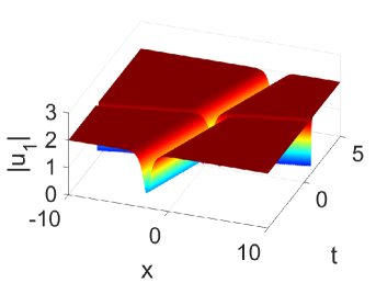
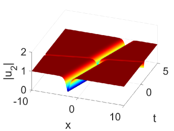
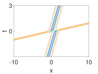
(1) Before collision, i.e., tt\rightarrow-\infty
Soliton 1 (ξ1+ξ10,ξ2+ξ2\xi_{1}+\xi^{*}_{1}\approx 0,\ \ \xi_{2}+\xi^{*}_{2}\rightarrow-\infty)

u1ρ1exp(iθ1)[12(1+A1)12(1A1)tanh(Re(ξ1)+12log(χ1))],\displaystyle u_{1}\rightarrow\rho_{1}\exp(\mathrm{i}\theta_{1})\left[\dfrac{1}{2}\left(1+A_{1}\right)-\dfrac{1}{2}\left(1-A_{1}\right)\tanh\left(\mathrm{Re}(\xi_{1})+\dfrac{1}{2}\mathrm{log}\left(\chi_{1}\right)\right)\right],
u2ρ2exp(iθ2)[12(1+B1)12(1B1)tanh(Re(ξ1)+12log(χ1))].\displaystyle u_{2}\rightarrow\rho_{2}\exp(\mathrm{i}\theta_{2})\left[\dfrac{1}{2}\left(1+B_{1}\right)-\dfrac{1}{2}\left(1-B_{1}\right)\tanh\left(\mathrm{Re}(\xi_{1})+\dfrac{1}{2}\mathrm{log}\left(\chi_{1}\right)\right)\right].

Soliton 2 (ξ2+ξ20,ξ1+ξ1+\xi_{2}+\xi^{*}_{2}\approx 0,\ \ \xi_{1}+\xi^{*}_{1}\rightarrow+\infty)

u1ρ1A1exp(iθ1)[12(1+A2)12(1A2)tanh(Re(ξ2)+12log(γ1))],\displaystyle u_{1}\rightarrow\rho_{1}A_{1}\mathrm{exp}(\mathrm{i}\theta_{1})\left[\dfrac{1}{2}\left(1+A_{2}\right)-\dfrac{1}{2}\left(1-A_{2}\right)\tanh\left(\mathrm{Re}(\xi_{2})+\dfrac{1}{2}\mathrm{log}\left(\gamma_{1}\right)\right)\right],
u2ρ2B1exp(iθ2)[12(1+B2)12(1B2)tanh(Re(ξ2)+12log(γ1))].\displaystyle u_{2}\rightarrow\rho_{2}B_{1}\mathrm{exp}(\mathrm{i}\theta_{2})\left[\dfrac{1}{2}\left(1+B_{2}\right)-\dfrac{1}{2}\left(1-B_{2}\right)\tanh\left(\mathrm{Re}(\xi_{2})+\dfrac{1}{2}\mathrm{log}\left(\gamma_{1}\right)\right)\right].

where the phases term in Soliton 1 and Soliton 2 was respectively expressed as

χ1=iIm(p1)Re(p1),γ1=iIm(p2)Re(p2)M.\chi_{1}=\mathrm{i}\dfrac{\mathrm{Im}(p_{1})}{\mathrm{Re}(p_{1})},\ \ \gamma_{1}=\mathrm{i}\dfrac{\mathrm{Im}(p_{2})}{\mathrm{Re}(p_{2})}M.

(2) After collision, i.e., t+t\rightarrow+\infty
Soliton 1 (ξ1+ξ10,ξ2+ξ2+\xi_{1}+\xi^{*}_{1}\approx 0,\ \ \xi_{2}+\xi^{*}_{2}\rightarrow+\infty)

u1ρ1A2exp(iθ1)[12(1+A1)12(1A1)tanh(Re(ξ1)+12log(χ2))],\displaystyle u_{1}\rightarrow\rho_{1}A_{2}\mathrm{exp}(\mathrm{i}\theta_{1})\left[\dfrac{1}{2}\left(1+A_{1}\right)-\dfrac{1}{2}\left(1-A_{1}\right)\tanh\left(\mathrm{Re}(\xi_{1})+\dfrac{1}{2}\mathrm{log}\left(\chi_{2}\right)\right)\right],
u2ρ2B2exp(iθ2)[12(1+B1)12(1B1)tanh(Re(ξ1)+12log(χ2))].\displaystyle u_{2}\rightarrow\rho_{2}B_{2}\mathrm{exp}(\mathrm{i}\theta_{2})\left[\dfrac{1}{2}\left(1+B_{1}\right)-\dfrac{1}{2}\left(1-B_{1}\right)\tanh\left(\mathrm{Re}(\xi_{1})+\dfrac{1}{2}\mathrm{log}\left(\chi_{2}\right)\right)\right].

Soliton 2 (ξ2+ξ20,ξ1+ξ1\xi_{2}+\xi^{*}_{2}\approx 0,\ \ \xi_{1}+\xi^{*}_{1}\rightarrow-\infty)

u1ρ1exp(iθ1)[12(1+A2)12(1A2)tanh(Re(ξ2)+12log(γ2))],\displaystyle u_{1}\rightarrow\rho_{1}\exp(\mathrm{i}\theta_{1})\left[\dfrac{1}{2}\left(1+A_{2}\right)-\dfrac{1}{2}\left(1-A_{2}\right)\tanh\left(\mathrm{Re}(\xi_{2})+\dfrac{1}{2}\mathrm{log}\left(\gamma_{2}\right)\right)\right],
u2ρ2exp(iθ2)[12(1+B2)12(1B2)tanh(Re(ξ2)+12log(γ2))].\displaystyle u_{2}\rightarrow\rho_{2}\exp(\mathrm{i}\theta_{2})\left[\dfrac{1}{2}\left(1+B_{2}\right)-\dfrac{1}{2}\left(1-B_{2}\right)\tanh\left(\mathrm{Re}(\xi_{2})+\dfrac{1}{2}\mathrm{log}\left(\gamma_{2}\right)\right)\right].

where the phase term in Soliton 1 and Soliton 2 was respectively expressed as

χ2=iIm(p1)Re(p1)M,γ2=iIm(p2)Re(p2).\chi_{2}=\mathrm{i}\dfrac{\mathrm{Im}(p_{1})}{\mathrm{Re}(p_{1})}M,\ \ \gamma_{2}=\mathrm{i}\dfrac{\mathrm{Im}(p_{2})}{\mathrm{Re}(p_{2})}.

In Fig. 2, it can be found that a phase shift occurs after the solitons collide with each other due to the difference in phase terms χi\chi_{i} and γi\gamma_{i}. From the contour plot in Fig. 2, it is observed that the intensity of the dark solitons does not decrease after the collision.

5. Conclusion

In this paper, we derived the general dark-dark soliton solutions in the form of pfaffian for the ccmKdV equation (1.6)–(1.7) under nonzero boundary condition. This work solved an open problem existed for a long time. The crucial step is to link the two bilinear equations of the ccmKdV equaiton to the disrete BKP hierarchy through Miwa transformation. As future work, we will investigate the soliton solutions to the semi-discrete version of the ccmKdV equation and report the results elsewhere.

6. Appendix: Proof of the lemma 3.2

Proof.

By defining

(dm,i)=pimν=12(pi+aνpiaν)kνexpξi,\displaystyle(d_{m},i)=p^{m}_{i}\prod_{\nu=1}^{2}\left(\frac{p_{i}+a_{\nu}}{p_{i}-a_{\nu}}\right)^{k_{\nu}}\ \exp\xi_{i}\,, (6.1)

it is shown that the pfaffian elements in (3.1) satisfy the linear relations

x(i,j)\displaystyle\dfrac{\partial}{\partial x}(i,j) =(d1,i)(d0,j)(d0,i)(d1,j),\displaystyle=(d_{1},i)(d_{0},j)-(d_{0},i)(d_{1},j), (6.2)
(i,j)k1+1(i,j)\displaystyle(i,j)_{k_{1}+1}-(i,j) =(d0,j)k1+1(d0,i)(d0,j)(d0,i)k1+1.\displaystyle=(d_{0},j)_{k_{1}+1}(d_{0},i)-(d_{0},j)(d_{0},i)_{k_{1}+1}. (6.3)

Here we omit without changing terms, for example,

(i,j)k1+1=(i,j)k1+1,k2,(i,j)=(i,j)k1,k2,(d0,i)=(d0,i)k1,k2.(i,j)_{k_{1}+1}=(i,j)_{k_{1}+1,k_{2}},\ \ (i,j)=(i,j)_{k_{1},k_{2}},\ \ (d_{0},i)=(d_{0},i)_{k_{1},k_{2}}.

We can also show

τk1+1,k2=(d0¯,d0,1,2,,2N),\displaystyle\tau_{k_{1}+1,k_{2}}=(\bar{d_{0}},d_{0},1,2,\cdots,2N), (6.4)
τk11,k2=(d0~,d0,1,2,,2N),\displaystyle\tau_{k_{1}-1,k_{2}}=(\tilde{d_{0}},d_{0},1,2,\cdots,2N), (6.5)

where (d0¯,k)=(d0,k)k1+1(\bar{d_{0}},k)=(d_{0},k)_{k_{1}+1}, (d0~,k)=(d0,k)k11(\tilde{d_{0}},k)=(d_{0},k)_{{k_{1}}-1} and (d0¯,d0)=(d0~,d0)=1.(\bar{d_{0}},d_{0})=(\tilde{d_{0}},d_{0})=1. Thus, we have

τk1+1,k2=τk1,k2+j=12N(1)j(d0,1,,j^,,2N)(d0,j)k1+1,\displaystyle\tau_{k_{1}+1,k_{2}}=\tau_{k_{1},k_{2}}+\sum_{j=1}^{2N}(-1)^{j}(d_{0},1,\cdots,\hat{j},\cdots,2N)(d_{0},j)_{k_{1}+1}\,, (6.6)
τk11,k2=τk1,k2+j=12N(1)j(d0,1,,j^,,2N)(d0,j)k11.\displaystyle\tau_{k_{1}-1,k_{2}}=\tau_{k_{1},k_{2}}+\sum_{j=1}^{2N}(-1)^{j}(d_{0},1,\cdots,\hat{j},\cdots,2N)(d_{0},j)_{k_{1}-1}\,. (6.7)

Utilizing the (6.6) and (6.7), we can arrive at

τk1+1,k2τk11,k2τk1,k2τk1,k2\displaystyle\tau_{k_{1}+1,k_{2}}\tau_{k_{1}-1,k_{2}}-\tau_{k_{1},k_{2}}\tau_{k_{1},k_{2}}
=τk1,k2j=12N(1)j(d0,1,,j^,,2N)[(d0,j)k1+1+(d0,j)k11]\displaystyle=\tau_{k_{1},k_{2}}\sum_{j=1}^{2N}(-1)^{j}(d_{0},1,\cdots,\hat{j},\cdots,2N)[(d_{0},j)_{k_{1}+1}+(d_{0},j)_{k_{1}-1}]
+1i<j2N(1)i+j(d0,1,,i^,,2N)(d0,1,,j^,,2N)\displaystyle+\sum_{{1\leq i<j\leq 2N}}(-1)^{i+j}(d_{0},1,\cdots,\hat{i},\cdots,2N)(d_{0},1,\cdots,\hat{j},\cdots,2N)
×[(d0,i)k1+1(d0,j)k11+(d0,i)k11(d0,j)k1+1]\displaystyle\times[(d_{0},i)_{k_{1}+1}(d_{0},j)_{k_{1}-1}+(d_{0},i)_{k_{1}-1}(d_{0},j)_{k_{1}+1}]
+j=12N(d0,1,,j^,,2N)2(d0,j)k1+1(d0,j)k11\displaystyle+\sum_{j=1}^{2N}(d_{0},1,\cdots,\hat{j},\cdots,2N)^{2}(d_{0},j)_{k_{1}+1}(d_{0},j)_{k_{1}-1}
=τk1,k2j=12N(1)j(d0,1,,j^,,2N)[(d0,j)k1+1+(d0,j)k11]\displaystyle=\tau_{k_{1},k_{2}}\sum_{j=1}^{2N}(-1)^{j}(d_{0},1,\cdots,\hat{j},\cdots,2N)[(d_{0},j)_{k_{1}+1}+(d_{0},j)_{k_{1}-1}]
+1i<j2N(1)i+j(d0,1,,i^,,2N)(d0,1,,j^,,2N)\displaystyle+\sum_{{1\leq i<j\leq 2N}}(-1)^{i+j}(d_{0},1,\cdots,\hat{i},\cdots,2N)(d_{0},1,\cdots,\hat{j},\cdots,2N)
×[(d0,j)k1+1(d0,k)k11+(d0,j)k11(d0,k)k1+12(d0,j)(d0,k)]\displaystyle\times[(d_{0},j)_{k_{1}+1}(d_{0},k)_{k_{1}-1}+(d_{0},j)_{k_{1}-1}(d_{0},k)_{k_{1}+1}-2(d_{0},j)(d_{0},k)]
+j=12N[(d0,1,,j^,,2N)(d0,j)]2\displaystyle+\sum_{j=1}^{2N}[(d_{0},1,\cdots,\hat{j},\cdots,2N)(d_{0},j)]^{2}

Here this identity (d0,j)k1+1(d0,j)k11=(d0,j)2(d_{0},j)_{k_{1}+1}(d_{0},j)_{k_{1}-1}=(d_{0},j)^{2} is used. Now, the last two items can be simplified. By using

(d0,i)k1+1(d0,j)k11+(d0,i)k11(d0,j)k1+12(d0,i)(d0,j)\displaystyle(d_{0},i)_{k_{1}+1}(d_{0},j)_{k_{1}-1}+(d_{0},i)_{k_{1}-1}(d_{0},j)_{k_{1}+1}-2(d_{0},i)(d_{0},j)
=(pj+a1pja1+pja1pj+a1pi+a1pia1pia1pi+a1)((i,j)δ2N+1i,j),i<j.\displaystyle=\left(\dfrac{p_{j}+a_{1}}{p_{j}-a_{1}}+\dfrac{p_{j}-a_{1}}{p_{j}+a_{1}}-\dfrac{p_{i}+a_{1}}{p_{i}-a_{1}}-\dfrac{p_{i}-a_{1}}{p_{i}+a_{1}}\right)((i,j)-\delta_{2N+1-i,j}),\ \ i<j. (6.8)

So, we have

τk1+1,k2τk11,k2τk1,k2τk1,k2\displaystyle\tau_{k_{1}+1,k_{2}}\tau_{k_{1}-1,k_{2}}-\tau_{k_{1},k_{2}}\tau_{k_{1},k_{2}}
=τk1,k2j=12N(1)j(d0,1,,j^,,2N)[(d0,j)k1+1+(d0,j)k11]\displaystyle=\tau_{k_{1},k_{2}}\sum_{j=1}^{2N}(-1)^{j}(d_{0},1,\cdots,\hat{j},\cdots,2N)[(d_{0},j)_{k_{1}+1}+(d_{0},j)_{k_{1}-1}]
+1i<j2N(1)i+j(d0,1,,i^,,2N)(d0,1,,j^,,2N)\displaystyle+\sum_{{1\leq i<j\leq 2N}}(-1)^{i+j}(d_{0},1,\cdots,\hat{i},\cdots,2N)(d_{0},1,\cdots,\hat{j},\cdots,2N)
×(pj+a1pja1+pja1pj+a1pi+a1pia1pia1pi+a1)((i,j)δ2N+1i,j)\displaystyle\times\left(\dfrac{p_{j}+a_{1}}{p_{j}-a_{1}}+\dfrac{p_{j}-a_{1}}{p_{j}+a_{1}}-\dfrac{p_{i}+a_{1}}{p_{i}-a_{1}}-\dfrac{p_{i}-a_{1}}{p_{i}+a_{1}}\right)((i,j)-\delta_{2N+1-i,j})
=τk1,k2j=12N(1)j(d0,1,,j^,,2N)(pj+a1pja1+pja1pj+a1)(d0,j)\displaystyle=\tau_{k_{1},k_{2}}\sum_{j=1}^{2N}(-1)^{j}(d_{0},1,\cdots,\hat{j},\cdots,2N)\left(\dfrac{p_{j}+a_{1}}{p_{j}-a_{1}}+\dfrac{p_{j}-a_{1}}{p_{j}+a_{1}}\right)(d_{0},j)
+i=12Nj=12N(1)i+j1(d0,1,,i^,,2N)(d0,1,,j^,,2N)(pja1pj+a1+pj+a1pja1)(i,j)\displaystyle+\sum_{i=1}^{2N}\sum_{j=1}^{2N}(-1)^{i+j-1}(d_{0},1,\cdots,\hat{i},\cdots,2N)(d_{0},1,\cdots,\hat{j},\cdots,2N)\left(\dfrac{p_{j}-a_{1}}{p_{j}+a_{1}}+\dfrac{p_{j}+a_{1}}{p_{j}-a_{1}}\right)(i,j)
+j=1N(d0,1,,j^,,2N)(d0,1,,2N+1j^,,2N)\displaystyle+\sum_{j=1}^{N}(d_{0},1,\cdots,\hat{j},\cdots,2N)(d_{0},1,\cdots,\mathaccent 1371{2N+1-j},\cdots,2N)
×(p2N+1j+a1p2N+1ja1+p2N+1ja1p2N+1j+a1pj+a1pja1pja1pj+a1)\displaystyle\times\left(\dfrac{{p_{2N+1-j}}+a_{1}}{{p_{2N+1-j}}-a_{1}}+\dfrac{{p_{2N+1-j}}-a_{1}}{{p_{2N+1-j}}+a_{1}}-\dfrac{p_{j}+a_{1}}{p_{j}-a_{1}}-\dfrac{p_{j}-a_{1}}{p_{j}+a_{1}}\right)

and using

τk1,k2(d0,i)+j=12N(1)j1(d0,1,,j^,,2N)(i,j)=(d0,i,1,,2N)=0,\displaystyle\tau_{k_{1},k_{2}}(d_{0},i)+\sum_{j=1}^{2N}(-1)^{j-1}(d_{0},1,\cdots,\hat{j},\cdots,2N)(i,j)=(d_{0},i,1,\cdots,2N)=0, (6.9)

the sum of the first two terms vanished. Therefore,

τk1+1,k2τk11,k2τk1,k2τk1,k2\displaystyle\tau_{k_{1}+1,k_{2}}\tau_{k_{1}-1,k_{2}}-\tau_{k_{1},k_{2}}\tau_{k_{1},k_{2}}
=j=1N4a12(pj2p2N+1j2)(pj2a12)(p2N+1j2a12)(d0,1,,j^,,2N)(d0,1,,2N+1j^,,2N).\displaystyle=\sum_{j=1}^{N}\dfrac{4a^{2}_{1}(p_{j}^{2}-{p^{2}_{2N+1-j}})}{(p_{j}^{2}-a^{2}_{1})({p^{2}_{2N+1-j}}-a^{2}_{1})}(d_{0},1,\cdots,\hat{j},\cdots,2N)(d_{0},1,\cdots,\mathaccent 1371{2N+1-j},\cdots,2N). (6.10)

Similarly, we have

τk1,k2+1τk1,k21τk1,k2τk1,k2\displaystyle\tau_{k_{1},k_{2}+1}\tau_{k_{1},k_{2}-1}-\tau_{k_{1},k_{2}}\tau_{k_{1},k_{2}}
=j=1N4a22(pj2p2N+1j2)(pj2a22)(p2N+1j2a22)(d0,1,,j^,,2N)(d0,1,,2N+1j^,,2N).\displaystyle=\sum_{j=1}^{N}\dfrac{4a^{2}_{2}(p_{j}^{2}-{p^{2}_{2N+1-j}})}{(p_{j}^{2}-a^{2}_{2})({p^{2}_{2N+1-j}}-a^{2}_{2})}(d_{0},1,\cdots,\hat{j},\cdots,2N)(d_{0},1,\cdots,\mathaccent 1371{2N+1-j},\cdots,2N). (6.11)

By applying (6.2), we can further derive

xτk1,k2=(d0,d1,1,2,,2N),2x2τk1,k2=(d0,d2,1,2,,2N),\displaystyle\dfrac{\partial}{\partial x}\tau_{k_{1},k_{2}}=(d_{0},d_{1},1,2,\cdots,2N),\ \ \dfrac{\partial^{2}}{\partial x^{2}}\tau_{k_{1},k_{2}}=(d_{0},d_{2},1,2,\cdots,2N), (6.12)

where the pfaffian (d0,d1)=(d0,d2)=0(d_{0},d_{1})=(d_{0},d_{2})=0. Then

xτk1,k2=j=12N(1)j1(d0,1,,j^,,2N)(d1,j),\displaystyle\dfrac{\partial}{\partial x}\tau_{k_{1},k_{2}}=\sum_{j=1}^{2N}(-1)^{j-1}(d_{0},1,\cdots,\hat{j},\cdots,2N)(d_{1},j), (6.13)
2x2τk1,k2=j=12N(1)j1(d0,1,,j^,,2N)(d2,j).\displaystyle\dfrac{\partial^{2}}{\partial x^{2}}\tau_{k_{1},k_{2}}=\sum_{j=1}^{2N}(-1)^{j-1}(d_{0},1,\cdots,\hat{j},\cdots,2N)(d_{2},j). (6.14)

Through formulas (6.13) and (6.14), we can achieve

(x2τk1,k2)τk1,k2(xτk1,k2)2\displaystyle(\partial_{x}^{2}\tau_{k_{1},k_{2}})\tau_{k_{1},k_{2}}-(\partial_{x}\tau_{k_{1},k_{2}})^{2}
=τk1,k2[j=12N(1)j1(d0,1,,j^,,2N)(d2,j)][j=12N(1)j1(d0,1,,j^,,2N)(d1,j)]2\displaystyle=\tau_{k_{1},k_{2}}[\sum_{j=1}^{2N}(-1)^{j-1}(d_{0},1,\cdots,\hat{j},\cdots,2N)(d_{2},j)]-[\sum_{j=1}^{2N}(-1)^{j-1}(d_{0},1,\cdots,\hat{j},\cdots,2N)(d_{1},j)]^{2}
=τk1,k2j=12N(1)j1pj2(d0,1,,j^,,2N)(d0,j)[j=12N(1)j1(d0,1,,j^,,2N)(d1,j)]2\displaystyle=\tau_{k_{1},k_{2}}\sum_{j=1}^{2N}(-1)^{j-1}p_{j}^{2}(d_{0},1,\cdots,\hat{j},\cdots,2N)(d_{0},j)-[\sum_{j=1}^{2N}(-1)^{j-1}(d_{0},1,\cdots,\hat{j},\cdots,2N)(d_{1},j)]^{2}

the first term in the aforementioned equation can be simplified by applying (6.9),

=i=12Nj=12N(1)i+j1pi2(d0,1,,i^,,2N)(d0,1,,j^,,2N)(i,j)\displaystyle=\sum_{i=1}^{2N}\sum_{j=1}^{2N}(-1)^{i+j-1}p_{i}^{2}(d_{0},1,\cdots,\hat{i},\cdots,2N)(d_{0},1,\cdots,\hat{j},\cdots,2N)(i,j)
[j=12N(1)j1(d0,1,,j^,,2N)(d1,j)]2\displaystyle-[\sum_{j=1}^{2N}(-1)^{j-1}(d_{0},1,\cdots,\hat{j},\cdots,2N)(d_{1},j)]^{2}
=1i<j2N(1)i+j1(pi2pj2)(d0,1,,i^,,2N)(d0,1,,j^,,2N)(i,j)\displaystyle=\sum_{{1\leq i<j\leq 2N}}(-1)^{i+j-1}(p_{i}^{2}-p_{j}^{2})(d_{0},1,\cdots,\hat{i},\cdots,2N)(d_{0},1,\cdots,\hat{j},\cdots,2N)(i,j)
[j=12N(1)j1(d0,1,,j^,,2N)(d1,j)]2\displaystyle-[\sum_{j=1}^{2N}(-1)^{j-1}(d_{0},1,\cdots,\hat{j},\cdots,2N)(d_{1},j)]^{2}
=1i<j2N(1)i+j1(pi2pj2)(d0,1,,i^,,2N)(d0,1,,j^,,2N)δ2N+i1,j\displaystyle=\sum_{{1\leq i<j\leq 2N}}(-1)^{i+j-1}(p_{i}^{2}-p_{j}^{2})(d_{0},1,\cdots,\hat{i},\cdots,2N)(d_{0},1,\cdots,\hat{j},\cdots,2N)\delta_{2N+i-1,j}
+1i<j2N(1)i+j1(pi2pj2)(pipjpi+pj)(d0,1,,i^,,2N)(d0,1,,j^,,2N)(d0,i)(d0,j)\displaystyle+\sum_{{1\leq i<j\leq 2N}}(-1)^{i+j-1}(p_{i}^{2}-p_{j}^{2})(\dfrac{p_{i}-p_{j}}{p_{i}+p_{j}})(d_{0},1,\cdots,\hat{i},\cdots,2N)(d_{0},1,\cdots,\hat{j},\cdots,2N)(d_{0},i)(d_{0},j)
[j=12N(1)j1(d0,1,,j^,,2N)(d1,j)]2\displaystyle-[\sum_{j=1}^{2N}(-1)^{j-1}(d_{0},1,\cdots,\hat{j},\cdots,2N)(d_{1},j)]^{2}

Meanwhile, we can prove that the sum of the last two terms vanishes.

1i<j2N(1)i+j1(pipj)2(d0,1,,i^,,2N)(d0,1,,j^,,2N)(d0,i)(d0,j)\displaystyle\sum_{{1\leq i<j\leq 2N}}(-1)^{i+j-1}(p_{i}-p_{j})^{2}(d_{0},1,\cdots,\hat{i},\cdots,2N)(d_{0},1,\cdots,\hat{j},\cdots,2N)(d_{0},i)(d_{0},j)
[j=12N(1)j1(d0,1,,j^,,2N)(d1,j)]2\displaystyle-[\sum_{j=1}^{2N}(-1)^{j-1}(d_{0},1,\cdots,\hat{j},\cdots,2N)(d_{1},j)]^{2}
=1i<j2N(1)i+j1(pipj)2(d0,1,,i^,,2N)(d0,1,,j^,,2N)(d0,i)(d0,j)\displaystyle=\sum_{{1\leq i<j\leq 2N}}(-1)^{i+j-1}(p_{i}-p_{j})^{2}(d_{0},1,\cdots,\hat{i},\cdots,2N)(d_{0},1,\cdots,\hat{j},\cdots,2N)(d_{0},i)(d_{0},j)
j=12Npj2(d0,1,,j^,,2N)2(d0,j)2\displaystyle-\sum_{j=1}^{2N}p_{j}^{2}(d_{0},1,\cdots,\hat{j},\cdots,2N)^{2}(d_{0},j)^{2}
+21i<j2N(1)i+j1pipj(d0,1,,i^,,2N)(d0,1,,j^,,2N)(d0,i)(d0,j)\displaystyle+2\sum_{{1\leq i<j\leq 2N}}(-1)^{i+j-1}p_{i}p_{j}(d_{0},1,\cdots,\hat{i},\cdots,2N)(d_{0},1,\cdots,\hat{j},\cdots,2N)(d_{0},i)(d_{0},j)
=1i<j2N(1)i+j1(pi2+pj2)(d0,1,,i^,,2N)(d0,1,,j^,,2N)(d0,i)(d0,j)\displaystyle=\sum_{{1\leq i<j\leq 2N}}(-1)^{i+j-1}(p_{i}^{2}+p_{j}^{2})(d_{0},1,\cdots,\hat{i},\cdots,2N)(d_{0},1,\cdots,\hat{j},\cdots,2N)(d_{0},i)(d_{0},j)
j=12Npj2(d0,1,,j^,,2N)2(d0,j)2\displaystyle-\sum_{j=1}^{2N}p_{j}^{2}(d_{0},1,\cdots,\hat{j},\cdots,2N)^{2}(d_{0},j)^{2}
=12i=12Nj=12N(1)i+j1(d0,1,,i^,,2N)(d0,1,,j^,,2N)(d0,i)(d0,j)\displaystyle=\frac{1}{2}\sum_{i=1}^{2N}\sum_{j=1}^{2N}(-1)^{i+j-1}(d_{0},1,\cdots,\hat{i},\cdots,2N)(d_{0},1,\cdots,\hat{j},\cdots,2N)(d_{0},i)(d_{0},j)
=0\displaystyle=0

Thus, the left hand of the equation (3.11) can write as

2((x2τk1,k2)τk1,k2(xτk1,k2)2)\displaystyle 2((\partial_{x}^{2}\tau_{k_{1},k_{2}})\tau_{k_{1},k_{2}}-(\partial_{x}\tau_{k_{1},k_{2}})^{2})
=2×1i<j2N(1)i+j1(pi2pj2)(d0,1,,i^,,2N)(d0,1,,j^,,2N)δ2N+i1,j\displaystyle=2\times\sum_{{1\leq i<j\leq 2N}}(-1)^{i+j-1}(p_{i}^{2}-p_{j}^{2})(d_{0},1,\cdots,\hat{i},\cdots,2N)(d_{0},1,\cdots,\hat{j},\cdots,2N)\delta_{2N+i-1,j}
=2×j=1N(pj2p2N+1j2)(d0,1,,j^,,2N)(d0,1,,2N+j1^,,2N)\displaystyle=2\times\sum_{j=1}^{N}(p_{j}^{2}-{p^{2}_{2N+1-j}})(d_{0},1,\cdots,\hat{j},\cdots,2N)(d_{0},1,\cdots,\mathaccent 1371{2N+j-1},\cdots,2N)

Therefore, if relation is written as

2a12ρ12(pj2a12)(p2N+1j2a12)+2a22ρ22(pj2a22)(p2N+1j2a22)=1,\displaystyle\frac{2{a_{1}}^{2}{\rho_{1}}^{2}}{(p^{2}_{j}-a^{2}_{1})({p^{2}_{2N+1-j}}-a^{2}_{1})}+\frac{2{a_{2}}^{2}{\rho_{2}}^{2}}{(p^{2}_{j}-a^{2}_{2})({p^{2}_{2N+1-j}}-a^{2}_{2})}=-1,

we obtain the bilinear equation (3.11). ∎

Acknowledgements. Xiaochuan Liu’s research was supported by National Science Foundation of China (Grant No. 12271424).

References

  • [1]
  • [2] Y. Kodama, A. Hasegawa, Nonlinear pulse propagation in a monomode dielectric guide, IEEE J. Quantum Electron, 23 (1987), 510-524.
  • [3] A. Shabat, V. Zakharov,  Exact theory of two-dimensional self-focusing and one-dimensional self-modulation of waves in nonlinear media, Sov. Phys. JETP, 34 (1972), 62.
  • [4] V.E. Zakharov, A.B. Shabat, Interaction between solitons in a stable medium, Sov. Phys. JETP, 37 (1973), 823-828.
  • [5] M. Trippenbach, Y.B. Band, Effects of self-steepening and self-frequency shifting on short-pulse splitting in dispersive nonlinear media, Phys. Rev. A, 57 (1998), 4791.
  • [6] D.J. Kaup, A.C. Newell,  An exact solution for a derivative nonlinear Schrödinger equation, J. Math. Phys., 19 (1978), 798-801.
  • [7] H.H. Chen, Y.C. Lee, and C.S. Liu, Integrability of nonlinear Hamiltonian systems by inverse scattering method, Phys. Scr., 20 (1979), 490.
  • [8] R. Hirota, Exact envelope-soliton solutions of a nonlinear wave equation, J. Math. Phys., 14 (1973), 805-809.
  • [9] N. Sasa, J. Satsuma,  New-type of soliton solutions for a higher-order nonlinear Schrödinger equation, J. Phys. Soc. Jpn., 60 (1991), 409–417.
  • [10] G.P. Agrawal, Nonlinear fiber optics, Nonlinear Science at the Dawn of the 21st Century, Springer (2000), 195-211.
  • [11] C. Menyuk, Nonlinear pulse propagation in birefringent optical fibers, IEEE J. Quantum Electron., 23 (1987), 174-176.
  • [12] P.K.A. Wai, C.R. Menyuk, and H.H. Chen,  Effects of randomly varying birefringence on soliton interactions in optical fibers, Opt. Lett., 16 (1991), 1735-1737.
  • [13] C. Gilson, J. Hietarinta, J. Nimmo, and Y. Ohta, Sasa-Satsuma higher-order nonlinear Schrödinger equation and its bilinearization and multisoliton solutions, Phys. Rev. E, 68 (2003), 016614.
  • [14] R.S. Tasgal, M.J. Potasek, Soliton solutions to coupled higher-order nonlinear Schrödinger equations, J. Math. Phys., 33 (1992), 1208-1215.
  • [15] K. Porsezian, P.S. Sundaram, and A. Mahalingam, Coupled higher-order nonlinear Schrödinger equations in nonlinear optics: Painlevé analysis and integrability, Phys. Rev. E, 50 (1994), 1543.
  • [16] S.Y. Sakovich, T. Tsuchida, Symmetrically coupled higher-order nonlinear Schrödinger equations: singularity analysis and integrability, J. Phys. A: Math. Gen., 33 (2000), 7217.
  • [17] P. Wang, T.-P. Ma, and F.-H. Qi,  Analytical solutions for the coupled Hirota equations in the firebringent fiber, Appl. Math. Comput., 411 (2021), 126495.
  • [18] N. Liu, B. Guo,  Long-time asymptotics for the initial-boundary value problem of coupled Hirota equation on the half-line, Sci. China Math., 64 (2021), 81-110.
  • [19] Z.-Z. Kang, T.-C. Xia, Construction of multi-soliton solutions of the N-coupled Hirota equations in an optical fiber,Chin. Phys. Lett., 36 (2019), 110201.
  • [20] S. Chen, L. Song, Rogue waves in coupled Hirota systems, Phys. Rev. E, 87 (2013), 032910.
  • [21] X. Wang, Y. Li, and Y. Chen, Generalized Darboux transformation and localized waves in coupled Hirota equations, Wave Motion, 51 (2014), 1149-1160.
  • [22] Q.-H. Park, H. Shin, Higher order nonlinear optical effects on polarized dark solitons, Opt. Commun., 178 (2000), 233-244.
  • [23] S.G. Bindu, A. Mahalingam, and K. Porsezian, Dark soliton solutions of the coupled Hirota equation in nonlinear fiber, Phys. Lett. A, 286 (2001), 321-331.
  • [24] K. Porsezian, K. Nakkeeran, Optical solitons in birefringent fibre-Bäcklund transformation approach, Pure Appl. Opt., 6 (1997), L7.
  • [25] S. Chen, Dark and composite rogue waves in the coupled Hirota equations, Phys. Lett. A, 378 (2014), 2851-2856.
  • [26] X. Wang, Y. Chen, Rogue-wave pair and dark-bright-rogue wave solutions of the coupled Hirota equations, Chin. Phys. B, 23 (2014), 070203.
  • [27] T. Xu, X. Xu, Single-and double-hump femtosecond vector solitons in the coupled Sasa-Satsuma system, Phys. Rev. E, 87 (2013), 032913.
  • [28] X. Lü, Bright-soliton collisions with shape change by intensity redistribution for the coupled Sasa-Satsuma system in the optical fiber communications, Commun. Nonlinear Sci. Numer. Simul., 19 (2014), 3969-3987.
  • [29] L. Liu, B. Tian, H. Yin, and Z. Du,  Vector bright soliton interactions of the coupled Sasa-Satsuma equations in the birefringent or two-mode fiber, Commun. Math. Phys., 80 (2018), 91–101.
  • [30] L.-C. Zhao, Z.-Y. Yang, and L. Ling,  Localized waves on continuous wave background in a two-mode nonlinear fiber with high-order effects, J. Phys. Soc. Jpn., 83 (2014), 104401.
  • [31] H.-Q. Zhang, Y. Wang, and W.-X. Ma,  Binary Darboux transformation for the coupled Sasa-Satsuma equations, Chaos, 27 (2017)
  • [32] L. Liu, B. Tian, Y. Yuan, and Z. Du,  Dark-bright solitons and semirational rogue waves for the coupled Sasa-Satsuma equations, Phys. Rev. E, 97 (2018), 052217.
  • [33] X. Geng, J. Wu, Riemann-Hilbert approach and N-soliton solutions for a generalized Sasa-Satsuma equation, Wave Motion, 60 (2016), 62-72.
  • [34] Y. Liu, W.-X. Zhang, and W.-X. Ma,  Riemann-Hilbert problems and soliton solutions for a generalized coupled Sasa–Satsuma equation, Commun. Nonlinear Sci. Numer. Simul., 118 (2023), 107052.
  • [35] F. Wu, L. Huang, Riemann-Hilbert approach and N-soliton solutions of the coupled generalized Sasa-Satsuma equation, Nonlinear Dyn., 110 (2022), 3617-3627.
  • [36] X. Geng, J. Wu, Inverse scattering transform of the coupled Sasa-Satsuma equation by Riemann-Hilbert approach, Commun. Theor. Phys., 67 (2017), 527.
  • [37] G.Zhang, C. Shi, C. Wu, and B.-F. Feng, Dark Soliton and Breather Solutions to the Coupled Sasa-Satsuma Equation, J. Nonlinear Sci., 35 (2025), 7.
  • [38] G. Zhang, X. Chen, B.-F. Feng, and C. Wu,  Rogue wave solutions to the coupled Sasa-Satsuma equation, Physica D, (2025), 134549.
  • [39] C. Shi, B. Liu, and B.-F. Feng, General soliton solutions to the coupled Hirota equation via the Kadomtsev-Petviashvili reduction, arXiv preprint arXiv:2502.13088, 2025
  • [40] M. Iwao, R. Hirota Soliton solutions of a coupled modified KdV equations, J. Phys. Soc. Jpn., 66 (1997), 577-588.
  • [41] T. Tsuchida, M. Wadati,  The coupled modified Korteweg-de Vries equations, J. Phys. Soc. Jpn., 67 (1998), 1175-1187.
  • [42] X. Xu, Y. Yang,  Breather and nondegenerate solitons in the two-component modified Korteweg-de Vries equation, Appl. Math. Lett., 144 (2023), 108695.
  • [43] H.N. Chan, K.W. Chow,   Rogue waves for an alternative system of coupled Hirota equations: Structural robustness and modulation instabilities, Stud. Appl. Math., 139 (2017), 78-103.
  • [44] P. Adamopoulou, G. Papamikos,  Drinfel’d-Sokolov construction and exact solutions of vector modified KdV hierarchy, Nucl. Phys. B, 952 (2019), 114933.
  • [45] R. Hirota, The direct method in soliton theory, Cambridge University Press, 2004
  • [46] T. Miwa,  On Hirota’s difference equations, Proc. Japan Acad., Ser. A:Math. Sci., 58 (1982), 9-12.
  • [47] S. Tsujimoto, R. Hirota Pfaffian representation of solutions to the discrete BKP hierarchy in bilinear form, J. Phys. Soc. Jpn., 65 (1996), 2797-2806.
  • [48] B.-F. Feng, K.-i. Maruno, and Y. Ohta, Integrable semi-discretizations of the reduced Ostrovsky equation, J. Phys. A, 48 (2015), 135203.
  • [49] B.-F. Feng, X.-D. Luo, M.J. Ablowitz, and Z.H. Musslimani,  General soliton solution to a nonlocal nonlinear Schrödinger equation with zero and nonzero boundary conditions, Nonlinearity, 31 (2018), 5385.