Persistent spectral based machine learning (PerSpect ML) for drug design

Graph or network models have been applied to various material, chemical and biological systems. In these models, atoms and bonds are usually simplified as vertices and edges. Mathematically, a graph representation can be denoted as $G(V,E)$, where $V=\{v_{i};i=1,2,...,N\}$ are vertex set with $N=|V|$ the total number. Here $E=\{e_{i}=(v_{i_{1}},v_{i_{2}});1\leq i_{1}\leq N,1\leq i_{2}\leq N\}$ denotes the edge set.

A simplicial complex is the generalization of a graph into its higher-dimensional counterpart. The simplicial complex is composed of simplexes. Each simplex is a finite set of vertices, and can be viewed geometrically as, a point (0-simplex), an edge (1-simplex), a triangle (2-simplex), a tetrahedron (3-simplex), and their k-dimensional counterpart (k-simplex). More specifically, a $k$-simplex $\sigma^{k}=\{v_{0},v_{1},v_{2},\cdots,v_{k}\}$ is the convex hull formed by $k+1$ affinely independent points $v_{0},v_{1},v_{2},\cdots,v_{k}$ as follows,

$\displaystyle\sigma^{k}=\left\{\lambda_{0}v_{0}+\lambda_{1}v_{1}+\cdots+\lambda_{k}v_{k}\mid\sum^{k}_{i=0}\lambda_{i}=1;\forall i,0\leq\lambda_{i}\leq 1\right\}.$

The $i$-th dimensional face of $\sigma^{k}$ ($i<k$) is the convex hull formed by $i+1$ vertices from the set of $k+1$ points $v_{0},v_{1},v_{2},\cdots,v_{k}$. The simplexes are the basic components for a simplicial complex.

A simplicial complex $K$ is a finite set of simplexes that satisfy two conditions. Firstly, any face of a simplex from $K$ is also in $K$. Secondly, the intersection of any two simplexes in $K$ is either empty or a shared face. A $k$-th chain group $C_{k}$ is an Abelian group generated by oriented $k$-simplexes $\sigma^{k}$, which are simplexes together with an orientation, i.e., ordering of their vertex set. The boundary operator $\partial_{k}$ ($C_{k}\rightarrow C_{k-1}$) for an oriented $k$-simplex $\sigma^{k}$ can be denoted as,

$\displaystyle\partial_{k}\sigma^{k}=\sum^{k}_{i=0}(-1)^{i}[v_{0},v_{1},v_{2},\cdots,\hat{v_{i}},\cdots,v_{k}].$

Here $[v_{0},v_{1},v_{2},\cdots,\hat{v_{i}},\cdots,v_{k}]$ is a oriented $(k-1)$-simplex, which is generated by the original set of vertices except $v_{i}$. The boundary operator maps a simplex to its faces and it guarantees that $\partial_{k-1}\partial_{k}=0$.

To facilitate a better description, we use notation $\sigma_{j}^{k-1}\subset\sigma_{i}^{k}$ to indicate that $\sigma_{j}^{k-1}$ is a face of $\sigma_{i}^{k}$, and notation $\sigma_{j}^{k-1}\sim\sigma_{i}^{k}$ if they have the same orientation, i.e., oriented similarly. For two oriented $k$-simplexes, $\sigma_{i}^{k}$ and $\sigma_{j}^{k}$, of a simplicial complex $K$, they are upper adjacent, denoted as $\sigma_{i}^{k}\frown\sigma_{j}^{k}$, if they are faces of a common $(k+1)$-simplex; they are lower adjacent, denoted as $\sigma_{i}^{k}\smile\sigma_{j}^{k}$, if they share a common $(k-1)$-simplex as they face. Moreover, if the orientations (or signs) of their common lower simplex are the same, it is called similar common lower simplex ($\sigma_{i}^{k}\smile\sigma_{j}^{k}$ and $\sigma_{i}^{k}\sim\sigma_{j}^{k}$); if their orientations are differently, it is called dissimilar common lower simplex ($\sigma_{i}^{k}\smile\sigma_{j}^{k}$ and $\sigma_{i}^{k}\not\sim\sigma_{j}^{k}$). The (upper) degree of a $k$-simplex $\sigma_{i}^{k}$, denoted as $d(\sigma^{k})$, is the number of $(k+1)$-simplexes, of which $\sigma_{i}^{k}$ is a face.

A hypergraph is a generalization of graph in which an edge is made of a set of vertices. Mathematically, a hypergraph $H(V,E^{h})$ consists of a set of vertices (denoted as $V$), and a set of hyperedges (denoted as $E^{h}$). Each hyperedge contains an arbitrarily number of vertices, and can be regarded as a subset of $V$. A hyperedge $e_{i}^{h}$ is said to be incident with a vertex $v_{j}$, when the vertice is in the hyperedge, i.e., $v_{j}\in e_{i}^{h}$. Note that a hypergraph can also be viewed as a generalization of simplicial complex.

An illustration of graph, simplicial complex and hypergraph can be found in Figure 1. These topological representations are made from the same set of vertices, but they characterize different topological connections.

In spectral graph theory, a graph $G(V,E)$ is represented by its adjacency matrix and Laplacian matrix [11, 39, 26, 44]. The adjacency matrix ${\bf A}$ describes the connectivity information and can be expressed as,

$\displaystyle A(i,j)=\begin{cases}\begin{array}[]{ll}1,&(v_{i},v_{j})\in E\\ 0,&(v_{i},v_{j})\not\in E.\\ \end{array}\end{cases}$

The degree of a vertex $v_{i}$ is the total number of edges that are connected to vertex $v_{i}$, i.e., $d(v_{i})=\sum_{i\neq j}^{N}A(i,j)$. The vertex diagonal matrix ${\bf D}$ can be defined as,

$\displaystyle D(i,j)=\begin{cases}\begin{array}[]{ll}\sum_{i\neq j}^{N}A(i,j),&i=j\\ 0,&i\neq j.\end{array}\end{cases}$

Laplacian matrix, also known as admittance matrix and Kirchhoff matrix, is defined as ${\bf L}={\bf D}-{\bf A}$. More specifically, it can be expressed as,

$\displaystyle L(i,j)=\begin{cases}\begin{array}[]{ll}d(v_{i}),&i=j\\ -1,&i\neq j~{}{\rm and}~{}(v_{i},v_{j})\in E\\ 0,&i\neq j~{}{\rm and}~{}(v_{i},v_{j})\not\in E.\end{array}\end{cases}$

(1)

The Laplacian matrix has many important properties. It is always positive-semidefinite, thus all its eigenvalues are non-negative. In particular, the number (multiplicity) of zero eigenvalues equals to an topological invariant, known as $\beta_{0}$, which counts the number of connected components in the graph. The second smallest eigenvalue, i.e., the first non-zero eigenvalue, is called Fiedler value or algebraic connectivity, which describes the general connectivity of the graph. The corresponding eigenvector can be used to subdivide the graph into two well-connected subgraphs. All eigenvalues and eigenvectors form an eigen spectrum and spectral graph theory studies the properties of the graph eigen spectrum.

There are two types of normalized Laplacian matrixes, including the symmetric normalized Laplacian matrix, which is defined as ${\bf L}_{\text{sym}}={\bf D}^{-1/2}{\bf L}{\bf D}^{-1/2}$, and random walk normalized Laplacian, which is defined as ${\bf L}_{\text{rw}}={\bf D}^{-}{\bf L}$.

The spectral simplicial complex theory studies the spectral properties of combinatorial Laplacian (or Hodge Laplacian) matrixes, that are constructed based on a simplicial complex [13, 27, 18, 2, 28, 36, 38, 43].

For an oriented simplicial complex, its $k$-th boundary (or incidence) matrix ${\bf B}_{k}$ can be defined as follows,

$\displaystyle B_{k}(i,j)=\left\{\begin{array}[]{ll}1,&\text{if }\sigma_{i}^{k-1}\subset\sigma_{j}^{k}~{}\text{and }~{}\sigma_{i}^{k-1}\sim\sigma_{j}^{k}\\ -1,&\text{if }\sigma_{i}^{k-1}\subset\sigma_{j}^{k}~{}\text{and }~{}\sigma_{i}^{k-1}\not\sim\sigma_{j}^{k}\\ 0,&\text{if }\sigma_{i}^{k-1}\not\subset\sigma_{j}^{k}.\end{array}\right.$

(5)

These boundary matrixes satisfy the condition that ${\bf B}_{k}{\bf B}_{k+1}={\bf 0}$. The $k$-th combinatorial Laplacian matrix can be expressed as follows,

$\displaystyle{\bf L}_{k}={\bf B}^{T}_{k}{\bf B}_{k}+{\bf B}_{k+1}{\bf B}^{T}_{k+1}.$

Note that $0$-th combinatorial Laplacian is,

$${\bf L}_{0}={\bf B}_{1}{\bf B}^{T}_{1}.$$

Further, if the highest order of the simplicial complex $K$ is $n$, then the $n$-th combinatorial Laplacian matrix is ${\bf L}_{n}={\bf B}^{T}_{n}{\bf B}_{n}$.

The above combinatorial Laplacian matrixes can be explicitly described in terms of the simplex relations. More specifically, ${\bf L}_{0}$, i.e., when $k=0$, can be expressed as,

$\displaystyle L_{0}(i,j)=\left\{\begin{array}[]{ll}d(\sigma_{i}^{0}),&\text{if }i=j\\ -1,&\text{if }i\neq j~{}\text{and }\sigma_{i}^{0}\frown\sigma_{j}^{0}\\ 0,&\text{if }i\neq j~{}\text{and }\sigma_{i}^{0}\not\frown\sigma_{j}^{0}.\end{array}\right.$

(9)

It can be seen that this expression is exactly the graph Laplacian as in Eq. (1). Further, when $k>0$, ${\bf L}_{k}$ can be expressed as [27],

$\displaystyle L_{k}(i,j)=\left\{\begin{array}[]{l}d(\sigma_{i}^{k})+k+1,\quad\text{if }i=j\\ 1,\qquad\text{if }i\neq j,\sigma_{i}^{k}\not\frown\sigma_{j}^{k},\sigma_{i}^{k}\smile\sigma_{j}^{k}~{}\text{and }\sigma_{i}^{k}\sim\sigma_{j}^{k}\\ -1,\quad\text{if }i\neq j,\sigma_{i}^{k}\not\frown\sigma_{j}^{k},\sigma_{i}^{k}\smile\sigma_{j}^{k}~{}\text{and }\sigma_{i}^{k}\not\sim\sigma_{j}^{k}\\ 0,\qquad\text{if }i\neq j,\sigma_{i}^{k}\frown\sigma_{j}^{k}~{}\text{or }~{}\sigma_{i}^{k}\not\smile\sigma_{j}^{k}.\end{array}\right.$

(14)

The eigenvalues of combinatorial Laplacian matrixes are independent of the choice of the orientation [18]. Further, the multiplicity of zero eigenvalues, i.e., the total number of zero eigenvalues, of ${\bf L}_{k}$ equals to the $k$-th Betti number $\beta_{k}$. Geometrically, $\beta_{0}$ is the number of connected components, $\beta_{1}$ is the number of circles or loops, and $\beta_{2}$ is the number of voids or cavities.

We can define the $k$-th combinatorial down Laplacian matrix as ${\bf L}^{\text{down}}_{k}={\bf B}^{T}_{k}{\bf B}_{k}$ and combinatorial up Laplacian matrix as ${\bf L}^{\text{up}}_{k}={\bf B}_{k+1}{\bf B}^{T}_{k+1}$. These matrixes have very interesting spectral properties [2]. Firstly, eigenvectors associated nonzero eigenvalues of ${\bf L}^{\text{down}}_{k}$ are orthogonal to eigenvectors from nonzero eigenvalues of ${\bf L}^{\text{up}}_{k}$; Secondly, nonzero eigenvalues of of ${\bf L}_{k}$ are either the eigenvalues of ${\bf L}^{\text{down}}_{k}$ or those of ${\bf L}^{\text{up}}_{k}$; Thirdly, eigenvectors associated with nonzero eigenvalues of ${\bf L}_{k}$ are either eigenvectors of ${\bf L}^{\text{down}}_{k}$ or those of ${\bf L}^{\text{up}}_{k}$.

Laplacian matrixes can also be defined on hypergraph [16, 42, 12, 25, 3]. One way to do that is to employ a clique expansion, in which a graph is construct from a hypergraph $H(V,E)$ by replacing each hyperedge with an edge for each pair of vertices in this hyperedge. A graph Laplacian matrix can then be defined on this hypergraph-induced graph. Note that the clique expansion also generate a clique complex, and combinatorial Laplacian matrixes can also be constructed based on it.

The other way is to directly use the incidence matrix. In a hypergraph, an incidence matrix $\bf H$ can be defined as follows,

$\displaystyle H(i,j)=\left\{\begin{array}[]{ll}1,&\text{if }v_{i}\in e^{h}_{j}\\ 0,&\text{if }v_{i}\not\in e^{h}_{j}.\end{array}\right.$

(17)

The vertex diagonal matrix ${\bf D}_{v}$ is,

$\displaystyle D_{v}(i,j)=\begin{cases}\begin{array}[]{ll}\sum_{j}H(i,j),&i=j\\ 0,&i\neq j.\end{array}\end{cases}$

The hypergraph adjacent matrix is then defined as ${\bf A}={\bf H}{\bf H}^{T}-{\bf D}_{v}$. And the unnormalized hypergraph Laplacian matrix is defined as,

$\displaystyle{\bf L}=2{\bf D}_{v}-{\bf H}{\bf H}^{T}.$

Similar to the graph models, the symmetric normalized hypergraph Laplacian is defined as ${\bf L}_{\text{sym}}=2{\bf I}-{\bf D}^{-1/2}_{v}{\bf H}{\bf H}^{T}{\bf D}^{-1/2}_{v}$ with ${\bf I}$ the identity matrix. The random walk hypergraph Laplacian is defined as ${\bf L}_{\text{rw}}=2{\bf I}-{\bf D}^{-1}_{v}{\bf H}{\bf H}^{T}$.

A filtration process naturally generates a mutliscale representation [14]. Filtration parameter, denoted as $f$ and key to the filtration process, is usually chosen as sphere radius (or diameter) for point cloud data, edge weight for graphs, and isovalue (or level set value) for density data. A systematical increase (or decrease) of the value for the filtration parameter will induce a sequence of hierarchical topological representations, which can be not only simplicial complexes, but also graphs and hypergraphs. For instance, a filtration operation on a distance matrix, i.e., a matrix with distances between any two vertices as its entries, can be defined by using a cutoff value as the filtration parameter. More specifically, if the distance between two vertices is smaller than the cutoff value, an edge is formed between them. In this way, a systematical increase (or decrease) of the cutoff value will deliver a series of nested graphs, with the graph produced at a lower cutoff value as a part (or a subset) of the graph produced at a larger cutoff value. Similarly, nested simplicial complexes can be constructed by using various definitions of complexes, such as Vietoris-Rips complex, $\check{C}$ech complex, Alpha complex, cubical complex, Morse complex, etc. Nested hypergraphs can also be generated by using a suitable definition of hyperedge.

The essential idea of our PerSpect theory is to provide a new mathematical representation that characterize the intrinsic topological and geometric information of the data. Different from all previous spectral models, our PerSpect theory considers not the eigen spectrum information of the graph, simplicial complex or hypergraph, constructed from a data at a particular scale, instead they focus on the variation of the eigen spectrum of these topological representations during a filtration process. Stated differently, our PerSpect theory studies the change of eigen spectrum in an “evolution” process, during which the structure of graph, simplicial complex or hypergraph “evolves” from a set of isolated vertices to a fully-connected topology, according to their inner structure connectivity and a predefined filtration parameter.

Mathematically, a filtration operation will deliver a nested sequence of graphs as follows,

$\displaystyle G^{0}\subseteq G^{1}\subseteq\cdots\subseteq G^{m}.$

Here $i$-th graph $G^{i}$ is generated at a certain filtration value $f_{i}$. Computationally, we can equally divide the filtration region (of the filtration parameter) into $m$ intervals and consider topological representations at each interval. A series of Laplacian matrixes $\{{\bf L}^{i}|_{i=1,2,...,m}\}$ can be generated from these graphs. Further, a nested sequence of simplicial complexes can also be generated from a filtration process,

$\displaystyle K^{0}\subseteq K^{1}\subseteq\cdots\subseteq K^{m}.$

Similarly, the $i$-th simplicial complex $K^{i}$ is generated at filtration value $f_{i}$. Combinatorial Laplacian matrix series $\{{\bf L}^{i}_{k}|_{i=1,2,...,m;k=0,1,2,...}\}$ can be constructed from these simplicial complexes. Note that the size of these Laplacian matrixes may be different. Moreover, with a suitable filtration process, a nested sequence of hypergraph can be generated as follows,

$\displaystyle H^{0}\subseteq H^{1}\subseteq\cdots\subseteq H^{m}.$

Hypergraph Laplacian matrix series $\{{\bf L}^{i}|_{i=1,2,...,m}\}$ can be constructed accordingly.

PerSpect theory studies the variation of the spectral information from the series of Laplacian matrixes. PerSpect variables and functions can be defined on the series of eigen spectrums. These PerSpect variables can incorporate both geometric and topological information in them. For instance, the multiplicity (or number) of $\text{Dim}(k)$ zero eigenvalues equals to Betti number $\beta_{k}$, thus persistent multiplicity, which is defined as the multiplicity of $\text{Dim}(k)$ zero eigenvalues over a filtration process, is exactly the Persistent Betti number or Betti curve. Further, we can consider the basic statistic properties, such as mean, standard deviation, maximum and minimum, of all non-zero eigenvalues, and define four other PerSpect variables, i.e., persistent mean, persistent standard deviation, persistent maximum and persistent minimum. Other spectral information, including algebraic connectivity, modularity, Cheeger constant, vertex/edge expansion, and other flow, random walk, and heat kernel related properties, can also be generalized into their corresponding PerSpect variables or functions.

As an illustration, we consider a PerSpect simplicial complex model of fullerene C₆₀. We choose cutoff distance as filtration parameter and use Vietoris-Rips complex to construct simplicial complex. Figure 2 demonstrates the generated sequence of nested simplicial complexes and their corresponding combinatorial Laplacian matrixes. Notation $\text{Dim}(k)$ means the $k$-th dimension, and only Laplacian matrixes at $\text{Dim}(0)$ to $\text{Dim}(2)$ are illustrated. It can be seen that, during the filtration process, complexes have been systematically generated and the simplicial complex evolve from a set with isolated vertices to a fully-connected complete topology. The corresponding Laplacian matrixes characterize this evolution process very well. For $\text{Dim}(0)$, at the very start of the filtration, there are only 60 vertices (0-simplex), thus a 60*60 all-zero ${\bf L}_{0}$ Laplacian matrix is generated. As the increase of filtration value, the size of ${\bf L}_{0}$ matrix remains unchanged, while more and more -1 value appears at its off-diagonal part. When the filtration value is large enough, a complete graph is obtained, and a full ${\bf L}_{0}$ matrix, i.e., all diagonal entries are 60 and off-diagonal entries are -1, is generated according to Eq.(9). For $\text{Dim}(1)$, at early stage of filtration, there exists no edges (1-simplexes) thus no ${\bf L}_{1}$ Laplacian matrices. With edges emerging as the filtration value increases, ${\bf L}_{1}$ matrixes are generated. Different from the $\text{Dim}(0)$ case, the size of ${\bf L}_{1}$ matrix increases systematically with the number of edges. Off-diagonal entries have both value 1 and -1 due to the orientation of the edge. When the filtration value is large enough, all edges will be either upper adjacent or not lower adjacent, thus ${\bf L}_{0}$ matrix becomes a diagonal matrix with all its diagonal entry value as 60, according to Eq.(14). For $\text{Dim}(2)$, no ${\bf L}_{2}$ Laplacian matrixes exist at the beginning stage of filtration, as no 2-simplexes are generated. The size of ${\bf L}_{2}$ matrixes also increases with the filtration and eventually evolve into a diagonal matrix with its diagonal entries all as 60 according to Eq.(14). Mathematically, higher dimensional Laplacian matrixes can also be systematically generated.

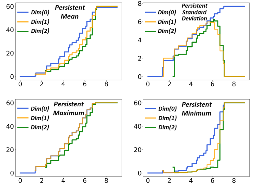Further, we can study PerSpect variables for fullerene C₆₀. Figure 3 shows the comparison between persistent barcode and persistent multiplicity. It can be seen that the persistent multiplicity is equivalent to the persistent Betti function [53], defined as the summation of persistent barcodes. In this way, the persistent homology information is naturally embedded into persistent multiplicity. Figure 4 shows the persistent mean, persistent standard deviation, persistent maximum and persistent minimum for C₆₀. It can be seen that these PerSpect variables change with the filtration value. Each variation of PerSpect variables indicates a certain change of the simplicial complex. At filtration size 7.10 Å, a complete simplicial complex is achieved, i.e., any $k+1$ vertices will form a $k$-simplex. The corresponding ${\bf L}_{0}$ has eigenvalues 0 (with multiplicity 1) and 60 (with multiplicity 59). The size for the corresponding ${\bf L}_{1}$ is 1770*1770, and its eigenvalues are all 60 (with multiplicity 1770). The size for complete corresponding ${\bf L}_{2}$ is 34220*34220, and its eigenvalues are also 60 (with multiplicity 34220).

Essentially, our PerSpect theory provides a mathematical representation of data, thus can work as a featurization for machine learning models. More specifically, PerSpect variables and functions can be discretized into feature vectors for different learning models. Other than the multiplicity of zero eigenvalues and non-zero eigenvalue statistic properties as mentioned above, spectral indexes from molecular descriptors can also be considered [37]. For a Laplacian matrix with eigenvalues $\{\lambda_{1},\lambda_{2},...,\lambda_{n}\}$, commonly-used spectral indexes include, sum of eigenvalues (Laplacian graph energy), sum of absolute deviation of eigenvalues (generalized average graph energy $\sum_{i=1}^{n}{\left|\lambda_{i}-\bar{\lambda}\right|}$ with $\bar{\lambda}$ the average eigenvalue), spectral moments ($\sum_{i=1}^{n}{{\lambda_{i}}^{k}}$ with $k$ the order of moment), quasi-Wiener index ($\sum_{j=1}^{A}{\frac{A+1}{\lambda_{j}}}$ with $\lambda_{j}>0$ and $A$ the number of all nonzero eigenvalues), spanning tree number ($\lg{[\frac{1}{A+1}\cdot\prod_{j=1}^{A}{\lambda_{j}}]}$), etc. Different from previous spectral index based molecular descriptors, which are extracted from a specific graph structure, a series of spectral index, i.e., an index vector, are considered from graphs, simplicial complexes, or hypergraphs obtained from the filtration process. Another potential featurization representation is to construct two dimensional (2D) images from these PerSpect variables [5]. The image representation will be more suitable for deep learning models.

Mathematical representations, that characterize biomolecular structural, physical, chemical and biological properties, are key to the success of machine learning models for drug design. For PerSpect ML based drug design, we consider element-specific (ES) biomolecular topological modeling [5]. Instead of using biomolecular topologies from either all-atom models or coarse-grained models (such as C_α), we decompose a biomolecule into different point sets, each with only one type of atoms, and construct topological representations for each set. For instance, a protein structure can be decomposed into 5 different points sets, that contain hydrogen(H), carbon(C), nitrogen(N), oxygen(O), and sulfur(S), separatively. Ligands are usually composed of totally 10 types of points sets, with the other 5 types of atoms including phosphorus(P), fluoride(F), chloride(Cl), bromide(Br) and iodine(I), respectively. Our PerSpect models can be employed on each set or each pair of atom sets. In this way, a detailed topological characterization of the biomolecular structure is obtained.

Further, for protein-ligand binding affinity prediction, we consider the interactive distance matrix (IDM) defined as follows [5],

$\displaystyle{M}(i,j)=\left\{\begin{array}[]{ll}{\scriptstyle\|{\bf r}_{i}-{\bf r}_{j}\|},&\text{if~{}}{\scriptstyle{\bf r}_{i}\in{\bf R}_{P},{\bf r}_{j}\in{\bf R}_{L}~{}\text{or}~{}{\bf r}_{i}\in{\bf R}_{L},{\bf r}_{j}\in{\bf R}_{P}}\\ {\infty},&\text{otherwise}.\end{array}\right.$

(19)

Here ${\bf r}_{i}$ and ${\bf r}_{j}$ are coordinates for the $i$- and $j$-th atoms, and $\|{\bf r}_{i}-{\bf r}_{j}\|$ is their Euclidean distance. Two sets ${\bf R}_{P}$ and ${\bf R}_{L}$ are atom coordinate sets for protein and ligand respectively. Only connections (or interactions) between protein atoms and ligand atoms are considered. Connections between atoms within either protein or ligand are ignored by setting their distance as $\infty$, i.e., an infinity large value. Element-specific interactive distance matrixes (ES-IDM) are considered for protein-ligand binding affinity prediction. That is to say there are totally 4*9=36 types of matrixes between 4 types of atoms from protein, including C, N, O, and S, and 9 types of atoms from ligand, including C, N, O, S, P, F, Cl, Br and I.

To characterize electrostatic properties, the interactive electrostatic matrix (IEM) is defined as follows [5],

$\displaystyle M_{E}(i,j)=\left\{\begin{array}[]{ll}\frac{1}{1+\exp({-\frac{cq_{i}q_{j}}{\|{\bf r}_{i}-{\bf r}_{j}\|}})},&\text{if~{}}{\scriptstyle{\bf r}_{i}\in{\bf R}_{P},{\bf r}_{j}\in{\bf R}_{L}~{}\text{or}~{}{\bf r}_{i}\in{\bf R}_{L},{\bf r}_{j}\in{\bf R}_{P}}\\ {\infty},&\text{otherwise}.\end{array}\right.$

(21)

Here $q_{i}$ and $q_{j}$ are partial charges for the $i$-th and $j$-th atoms, parameter $c$ is constant value. In our calculation $c$ is set to be 100. In this matrixes, electrostatic interactions between atoms within either protein or ligand are dismissed by setting their value as ${\infty}$. Only interactions between protein and ligand are considered. For element-specific interactive electrostatic matrix (ES-IEM), there are totally 5*10=40 types, between 5 types of atoms from protein, including H, C, N, O, and S, and 10 types of atoms from ligand, including H, C, N, O, S, P, F, Cl, Br and I.

References

- [1] K. Afifi and A. F. Al-Sadek. Improving classical scoring functions using random forest: The non-additivity of free energy terms’ contributions in binding. Chemical biology & drug design, 92(2):1429–1434, 2018.
- [2] S. Barbarossa and S. Sardellitti. Topological signal processing over simplicial complexes. arXiv preprint arXiv:1907.11577, 2019.
- [3] Sergio Barbarossa and Mikhail Tsitsvero. An introduction to hypergraph signal processing. In 2016 IEEE International Conference on Acoustics, Speech and Signal Processing (ICASSP), pp. 6425–6429. IEEE, 2016.
- [4] F. Boyles, C. Deane, and G. Morris. Learning from the ligand: using ligand-based features to improve binding affinity prediction. 2019.
- [5] Z. X. Cang, L. Mu, and G. W. Wei. Representability of algebraic topology for biomolecules in machine learning based scoring and virtual screening. PLoS computational biology, 14(1):e1005929, 2018.
- [6] Z. X. Cang and G. W. Wei. Analysis and prediction of protein folding energy changes upon mutation by element specific persistent homology. Bioinformatics, 33(22):3549–3557, 2017.
- [7] Z. X. Cang and G. W. Wei. Integration of element specific persistent homology and machine learning for protein-ligand binding affinity prediction. International journal for numerical methods in biomedical engineering, p. 10.1002/cnm.2914, 2017.
- [8] Z. X. Cang and G. W. Wei. TopologyNet: Topology based deep convolutional and multi-task neural networks for biomolecular property predictions. PLOS Computational Biology, 13(7):e1005690, 2017.
- [9] Z. X. Cang and G. W. Wei. Integration of element specific persistent homology and machine learning for protein-ligand binding affinity prediction. International journal for numerical methods in biomedical engineering, 34(2):e2914, 2018.
- [10] D. S. Cao, Q. S. Xu, Q. N. Hu, and Y. Z. Liang. ChemoPy: freely available python package for computational biology and chemoinformatics. Bioinformatics, 29(8):1092–1094, 2013.
- [11] F. Chung. Spectral graph theory. American Mathematical Society, 1997.
- [12] Joshua Cooper and Aaron Dutle. Spectra of uniform hypergraphs. Linear Algebra and its applications, 436(9):3268–3292, 2012.
- [13] B. Eckmann. Harmonische funktionen und randwertaufgaben in einem komplex. Commentarii Mathematici Helvetici, 17(1):240–255, 1944.
- [14] H. Edelsbrunner, D. Letscher, and A. Zomorodian. Topological persistence and simplification. Discrete Comput. Geom., 28:511–533, 2002.
- [15] E. N. Feinberg, D. Sur, Z. Q. Wu, B. E. Husic, H. H. Mai, Y. Li, S. S. Sun, J. Y. Yang, B. Ramsundar, and V. S. Pande. Potentialnet for molecular property prediction. ACS central science, 4(11):1520–1530, 2018.
- [16] K. Q. Feng and W. C. W. Li. Spectra of hypergraphs and applications. Journal of number theory, 60(1):1–22, 1996.
- [17] C. Grow, K. F. Gao, D. D. Nguyen, and G. W. Wei. Generative network complex (GNC) for drug discovery. arXiv preprint arXiv:1910.14650, 2019.
- [18] D. Horak and J. Jost. Spectra of combinatorial Laplace operators on simplicial complexes. Advances in Mathematics, 244:303–336, 2013.
- [19] J. Jiménez, M. Skalic, G. Martinez-Rosell, and G. De Fabritiis. KDEEP: Protein–ligand absolute binding affinity prediction via 3D-convolutional neural networks. Journal of chemical information and modeling, 58(2):287–296, 2018.
- [20] G. Landrum. RDKit: Open-source cheminformatics. 2006.
- [21] H. J. Li, K. S. Leung, M. H. Wong, and P. J. Ballester. Improving AutoDock Vina using random forest: the growing accuracy of binding affinity prediction by the effective exploitation of larger data sets. Molecular informatics, 34(2-3):115–126, 2015.
- [22] J. Liu and R. X. Wang. Classification of current scoring functions. Journal of chemical information and modeling, 55(3):475–482, 2015.
- [23] Z. H. Liu, Li Y., Han L., Liu J., Zhao Z. X., Nie W., Liu Y. C., and Wang R. X. PDB-wide collection of binding data: current status of the PDBbind database. Bioinformatics, 31(3):405–412, 2015.
- [24] Y. C. Lo, S. E. Rensi, W. Torng, and R. B. Altman. Machine learning in chemoinformatics and drug discovery. Drug discovery today, 23(8):1538–1546, 2018.
- [25] Linyuan Lu and Xing Peng. High-ordered random walks and generalized laplacians on hypergraphs. In International Workshop on Algorithms and Models for the Web-Graph, pp. 14–25. Springer, 2011.
- [26] B. Mohar, Y. Alavi, G. Chartrand, and O. R. Oellermann. The laplacian spectrum of graphs. Graph theory, combinatorics, and applications, 2(871-898):12, 1991.
- [27] A. Muhammad and M. Egerstedt. Control using higher order laplacians in network topologies. In Proc. of 17th International Symposium on Mathematical Theory of Networks and Systems, pp. 1024–1038. Citeseer, 2006.
- [28] S. Mukherjee and J. Steenbergen. Random walks on simplicial complexes and harmonics. Random structures & algorithms, 49(2):379–405, 2016.
- [29] D. D. Nguyen, Z. X. Cang, and G. W. Wei. A review of mathematical representations of biomolecular data. Physical Chemistry Chemical Physics, 2020.
- [30] D. D. Nguyen, Z. X. Cang, K. D. Wu, M. L. Wang, Y. Cao, and G. W. Wei. Mathematical deep learning for pose and binding affinity prediction and ranking in D3R Grand Challenges. Journal of computer-aided molecular design, 33(1):71–82, 2019.
- [31] D. D. Nguyen, Z. X. Cang, K. D. Wu, M. L. Wang, Y. Cao, and G. Wei. Wei. Mathematical deep learning for pose and binding affinity prediction and ranking in D3R Grand Challenges. Journal of computer-aided molecular design, 33(1):71–82, 2019.
- [32] D. D. Nguyen, K. F. Gao, M. L. Wang, and G. W. Wei. MathDL: Mathematical deep learning for D3R Grand Challenge 4. Journal of computer-aided molecular design, pp. 1–17, 2019.
- [33] D. D. Nguyen and G. W. Wei. AGL-Score: Algebraic graph learning score for protein-ligand binding scoring, ranking, docking, and screening. Journal of chemical information and modeling, 59(7):3291–3304, 2019.
- [34] D. D. Nguyen, T. Xiao, M. L. Wang, and G. W. Wei. Rigidity strengthening: A mechanism for protein–ligand binding. Journal of chemical information and modeling, 57(7):1715–1721, 2017.
- [35] N. M. O’Boyle, M. Banck, C. A. James, C. Morley, T. Vandermeersch, and G. R. Hutchison. Open Babel: An open chemical toolbox. Journal of cheminformatics, 3(1):33, 2011.
- [36] O. Parzanchevski and R. Rosenthal. Simplicial complexes: spectrum, homology and random walks. Random Structures & Algorithms, 50(2):225–261, 2017.
- [37] T. Puzyn, J. Leszczynski, and M. T. Cronin. Recent advances in QSAR studies: methods and applications, volume 8. Springer Science & Business Media, 2010.
- [38] S. Shukla and D. Yogeshwaran. Spectral gap bounds for the simplicial Laplacian and an application to random complexes. Journal of Combinatorial Theory, Series A, 169:105134, 2020.
- [39] D. A. Spielman. Spectral graph theory and its applications. In 48th Annual IEEE Symposium on Foundations of Computer Science (FOCS’07), pp. 29–38. IEEE, 2007.
- [40] M. M. Stepniewska-Dziubinska, P. Zielenkiewicz, and P. Siedlecki. Development and evaluation of a deep learning model for protein–ligand binding affinity prediction. Bioinformatics, 34(21):3666–3674, 2018.
- [41] M. Y. Su, Q. F. Yang, Y. Du, G. Q. Feng, Z. H. Liu, Y Li, and R. X. Wang. Comparative assessment of scoring functions: The CASF-2016 update. Journal of chemical information and modeling, 59(2):895–913, 2018.
- [42] Liang Sun, Shuiwang Ji, and Jieping Ye. Hypergraph spectral learning for multi-label classification. In Proceedings of the 14th ACM SIGKDD international conference on Knowledge discovery and data mining, pp. 668–676, 2008.
- [43] J. J. Torres and G. Bianconi. Simplicial complexes: higher-order spectral dimension and dynamics. arXiv preprint arXiv:2001.05934, 2020.
- [44] U. Von Luxburg. A tutorial on spectral clustering. Statistics and computing, 17(4):395–416, 2007.
- [45] B. Wang, C. Z. Wang, K. D. Wu, and G. W. Wei. Breaking the polar-nonpolar division in solvation free energy prediction. Journal of computational chemistry, 39(4):217–233, 2018.
- [46] B. Wang, Z. X. Zhao, and G. W. Wei. Automatic parametrization of non-polar implicit solvent models for the blind prediction of solvation free energies. The Journal of chemical physics, 145(12):124110, 2016.
- [47] R. Wang, D. D. Nguyen, and G. W. Wei. Persistent spectral graph. arXiv preprint arXiv:1912.04135, 2019.
- [48] G. W. Wei. Mathematics at the eve of a historic transition in biology. Computational and Mathematical Biophysics, 5(1), 2017.
- [49] G. W. Wei. Persistent homology analysis of biomolecular data. Journal of Computational Physics, 305:276–299, 2017.
- [50] M. Wójcikowski, M. Kukiełka, M. M. Stepniewska-Dziubinska, and P. Siedlecki. Development of a protein–ligand extended connectivity (PLEC) fingerprint and its application for binding affinity predictions. Bioinformatics, 35(8):1334–1341, 2019.
- [51] K. D. Wu and G. W. Wei. Quantitative toxicity prediction using topology based multi-task deep neural networks. Journal of chemical information and modeling, p. 10.1021/acs.jcim.7b00558, 2018.
- [52] K. D. Wu, Z. X. Zhao, R. X. Wang, and G. W. Wei. TopP–S: Persistent homology-based multi-task deep neural networks for simultaneous predictions of partition coefficient and aqueous solubility. Journal of computational chemistry, 39(20):1444–1454, 2018.
- [53] K. L. Xia, X. Feng, Y. Y. Tong, and G. W. Wei. Persistent homology for the quantitative prediction of fullerene stability. Journal of Computational Chemsitry, 36:408–422, 2015.
- [54] R. D. Zhao, Z. X. Cang, Y. Y. Tong, and G. W. Wei. Protein pocket detection via convex hull surface evolution and associated Reeb graph. Bioinformatics, 34(17):i830–i837, 2018.
- [55] L. Z. Zheng, J. R. Fan, and Y. G. Mu. OnionNet: a multiple-layer intermolecular-contact-based convolutional neural network for protein–ligand binding affinity prediction. ACS omega, 4(14):15956–15965, 2019.
- [56] A. Zomorodian and G. Carlsson. Computing persistent homology. Discrete Comput. Geom., 33:249–274, 2005.