Permutation-based tests for discontinuities in event studies††thanks: We thank the Coeditor and two anonymous referees for comments and suggestions that have greatly improved the manuscript.
Abstract
We propose using a permutation test to detect discontinuities in an underlying economic model at a known cutoff point. Relative to the existing literature, we show that this test is well suited for event studies based on time-series data. The test statistic measures the distance between the empirical distribution functions of observed data in two local subsamples on the two sides of the cutoff. Critical values are computed via a standard permutation algorithm. Under a high-level condition that the observed data can be coupled by a collection of conditionally independent variables, we establish the asymptotic validity of the permutation test, allowing the sizes of the local subsamples to be either be fixed or grow to infinity. In the latter case, we also establish that the permutation test is consistent. We demonstrate that our high-level condition can be verified in a broad range of problems in the infill asymptotic time-series setting, which justifies using the permutation test to detect jumps in economic variables such as volatility, trading activity, and liquidity. These potential applications are illustrated in an empirical case study for selected FOMC announcements during the ongoing COVID-19 pandemic.
KEYWORDS: event study, infill asymptotics, jump, permutation tests, randomization tests, semimartingale.
JEL classification codes: C12, C14, C22, C32.
1 Introduction
Many econometric problems can be expressed in terms of the continuity or the discontinuity of certain component in the underlying economic model. In an influential paper, Chow (1960) tested the temporal stability in the demand for automobiles, and subsequently stimulated a large literature on structural breaks in time series analysis; see, for example, Andrews (1993), Stock (1994), Bai and Perron (1998), and many references therein. In microeconometrics, the regression discontinuity design (RDD) has been extensively used for causal inference. This literature identifies and estimates an average treatment effect by evaluating discontinuities of conditional expectation functions of outcome and treatment variables at a cutoff point of the running variable; see Imbens and Lemieux (2008) and Lee and Lemieux (2010) for comprehensive reviews.111Coincidentally, the RDD was first proposed by Thistlethwaite and Campbell (1960) around the same time as the Chow test. Meanwhile, a more recent high-frequency financial econometrics literature has been devoted to studying discontinuities, or jumps, in various financial time series (e.g., price, volatility, trading activity, etc.). The high-frequency jump literature is pioneered by Barndorff-Nielsen and Shephard (2006), who propose the first nonparametric test for asset price jumps using high-frequency data in an infill asymptotic setting. More recently, Bollerslev et al. (2018) study the jumps of volatility and trading intensity in high-frequency jump regressions (Li et al. (2017)) that closely resemble the classical RDD.
Although these strands of literature involve apparently different terminology and technical tools, they share a common theme: The econometric goal is to learn about differences in the data generating processes between two subsamples separated by the cutoff. Imbens and Kalyanaraman (2011) emphasize that these subsamples should be “local” to the cutoff point, which is quite natural given the nonparametric nature of discontinuity inference (Hahn et al. (2001)). The issue under study is thus a local version of the classical two-sample problem. Correspondingly, the related inference is often carried out using nonparametric two-sample t-tests, which are based on kernel regressions in the RDD (Hahn et al. (2001), Imbens and Kalyanaraman (2011), Calonico et al. (2014)) or, in the same spirit, spot high-frequency estimators (Foster and Nelson (1996), Comte and Renault (1998), Jacod and Protter (2012), Li et al. (2017), Bollerslev et al. (2018)) in the infill time-series setting.
In an ideal scenario in which the subsamples separated by the cutoff are i.i.d. and independent of each other, the permutation test is an excellent tool to detect differences in their distributions. In particular, standard results for randomization inference (Lehmann and Romano (2005, Chapter 15.2)) indicate that a permutation test implemented with any arbitrary test statistic is finite-sample valid under these conditions. The recent literature has investigated the properties of permutation tests to detect differences between two samples under less ideal conditions. One example is Canay and Kamat (2017), who consider an RDD and show that permutation-based inference is asymptotically valid to detect discontinuities in the distribution of the baseline covariates at the cutoff. These authors implement their test with a finite number of observations that are located closest to the cutoff, effectively forcing them to concentrate on a small neighborhood of the cutoff as the sample size grows. In the same spirit, Cattaneo et al. (2017) propose using permutation-based inference to detect discontinuities at the cutoff under the “local randomization framework” introduced in Cattaneo et al. (2015). Outside of the RDD literature, Chung and Romano (2013) and DiCiccio and Romano (2017) investigate the asymptotic properties of permutation-based inference to test for differences in specific distributional features of two samples, such as the mean or the correlation coefficient. It is important to note that all of the references mentioned in this paragraph presume cross-sectional data.
In the context of time-series applications, there is an active literature on change-point tests implemented via permutations. This approach was first suggested by Antoch and Hušková (2001) and later pursued by other authors. See Hušková (2004) or Horváth and Rice (2014) for surveys of this literature. While most of this literature imposes independent errors, some allow for limited forms of weak dependence (Kirch and Steinebach (2006), Kirch (2007), and Jentsch and Pauly (2015)). In contrast, our econometric setting accommodates essentially unrestricted persistence and nonstationarity in the underlying state processes (e.g., volatility), which better suits our interest on their dynamics over short time windows around economic news events. In the context of machine-learning methods, Chernozhukov et al. (2018) propose using permutations to implement conformal inference that allows for time series data.
Set against this background, our main goal in this paper is to establish a general theory for permutation-based discontinuity tests, with a special emphasis on event studies based on time-series data. To capture the “local” nature of this problem, we adopt an infill asymptotic framework, under which the inference concentrates on observations “close” to the event time. Specifically, we consider the Cramér-von Mises test statistic formed as the squared distance between the empirical cumulative distribution functions for the two local subsamples near the cutoff, and compute the critical value via a standard permutation algorithm. As explained earlier, if the data were i.i.d., the behavior of this permutation test would follow directly from standard results for randomization inference. This “off-the-shelf” theory, however, is not applicable here because time-series data observed in a short event window can be serially highly dependent.
The main theoretical contribution of the present paper is to establish the asymptotic validity of the permutation test in this non-standard setting. The theory has two components. The first is a new general result for permutation test. Specifically, we link the (feasible) permutation test formed using the original data with an infeasible test constructed in a “coupling” problem that involves conditionally i.i.d. coupling variables. Since the latter resembles the classical two-sample problem, the infeasible test controls size exactly under the coupling null hypothesis (i.e., coupling variables in the two subsamples are homogeneous), and is consistent under the complementary alternative hypothesis. Under a proper notion of coupling, which is customized for the permutation test, we show that the feasible test inherits the same asymptotic rejection properties from the infeasible one. Since this result is of independent theoretical interest that is well beyond our subsequent analysis in the infill time-series setting, we frame the theory under general high-level conditions so as to facilitate other types of applications.
The second component of our analysis pertains to specializing the general result to the infill time-series setting designed for event-study applications. The event-study framework is particularly relevant for studying macroeconomic and financial shocks, including monetary shocks triggered by FOMC announcements (Cochrane and Piazzesi (2002), Nakamura and Steinsson (2018a)), or “natural disasters” such as the ongoing COVID-19 pandemic. Following Li and Xiu (2016) and Bollerslev et al. (2018), we model observed data using a general state-space framework, in which the observations are discretely sampled from a latent state process “contaminated” by random disturbances. This model has been used to model variables such as asset returns, trading volume, duration, and bid-ask spread, and readily accommodates both continuously and discretely valued variables. Under this state-space model, the temporal discontinuity in the data’s distribution is mainly driven by the jump of the latent state process (e.g., asset volatility, trading intensity, and propensity of informed trading), which can be detected by the permutation test. Under easy-to-verify primitive conditions, we construct coupling variables and apply the aforementioned general theory to establish the permutation test’s asymptotic validity.
We recognize two advantages of the proposed permutation test in comparison with the standard approach based on the nonparametric “spot” estimation of the underlying state process. Firstly, the permutation test attains asymptotic size control even if the number of observations in each subsample is fixed.222For similar type of results in the context of RDD; see Cattaneo et al. (2015), Cattaneo et al. (2017), Canay and Kamat (2017), and Bugni and Canay (2021). This remarkable property is reminiscent of the finite-sample exactness of the permutation test in the classical two-sample problem for i.i.d. data. In contrast, the nonparametric estimation approach works in a fundamentally different way, as it relies on the asymptotic (mixed) normality of the estimator, which in turn requires the sizes of the local subsamples to grow to infinity. In empirical applications, however, it is often desirable to use a short time window, either to reduce the effect of confounding factors in the background, or simply because of the lack of observations soon after the occurrence of the economic event (say, in a real-time research situation). Not surprisingly, the conventional inference based on asymptotic Gaussianity often results in large size distortions in this “small-sample” scenario, as we demonstrate concretely in a realistically calibrated Monte Carlo experiment (see Section 3). Meanwhile, the permutation test exhibits much more robust size control in finite samples.
The second advantage of the permutation test is its versatility: The same test can be applied in many different empirical contexts without any modification. On the other hand, the nonparametric estimation approach often relies on specific features of the problem, and needs to be designed on a case-by-case basis. Therefore, the proposed permutation test may be particularly attractive in new empirical environments for which tests based on the conventional approach are not yet developed or not yet well-understood. In Section 2.2, we illustrate this point more concretely in the context of testing for volatility jumps. In that case, the standard approach relies crucially on the assumption that the price shocks are Brownian in its design of the spot volatility estimator and the associated t-statistic, and it cannot be adapted easily to accommodate a more general setting with Lévy-driven shocks.333As explained by Barndorff-Nielsen and Shephard (2001), these more general processes offer the possibility of capturing important deviations from Brownian shocks and for flexible modelling of dependence structures. However, to the best of our knowledge, the estimation and inference of the spot volatility (i.e., the scaling process) in the non-Brownian case remains to be an open question in the literature. There is some limited work on the inference of integrated volatility functionals for the non-Brownian case (see Todorov and Tauchen (2012)) which demonstrates various distinct complications in the non-Brownian setting. The permutation test, on the other hand, is valid even in the latter, more general, setting.
That being said, we stress that the proposed permutation test is a complement, rather than substitute, for the conventional nonparametric estimation method, because it has two limitations. One is that the permutation test focuses exclusively on hypothesis testing, without producing a point estimate for the jump of the state process (e.g., volatility) of interest, whereas the estimate is a by-product of the conventional approach. In addition, the proposed permutation test is purely nonparametric and it does not exploit any parametric structure that one may be willing to impose. It is therefore conceivable that in certain semiparametric settings, more efficient tests may be designed to exploit a priori model restrictions. Put differently, the aforementioned versatility of the permutation test may come with an efficiency cost. A better understanding about the robustness-efficiency tradeoff might be an interesting topic for future research.
In an empirical illustration, we apply the permutation test to a recent sample of high-frequency intraday returns of the SPY ETF for the S&P 500 index. Specifically, we focus on four important FOMC announcements during the ongoing COVID-19 pandemic, and test whether each announcement induces discontinuities in volatility, trading activity, and two measures of market illiquidity. We document robust empirical evidence for discontinuities in volatility and trading activity. We also find evidence for announcement-induced discontinuity in transaction cost (measured by bid-ask spread), but not in market impact (gauged by Amihud’s measure). This application highlights one of the main advantages of the proposed test, namely, it is applicable for a broad variety of high-frequency observations modeled in distinct ways, which is unlike, for example, the conventional t-test designed specifically for testing volatility jumps in the Brownian setting.
The rest of the paper is organized as follows. We present the asymptotic theory for the permutation test in Section 2. Section 3 reports the test’s finite-sample performance in Monte Carlo experiments, and Section 4 presents the empirical illustration. Section 5 concludes. The appendix contains all proofs.
Notation. We use to denote the Euclidean norm of a vector . For any real number , we use to denote the smallest integer that is larger than . For any constant , denotes the norm for random variables. For two real sequences and , we write if for some finite constant .
2 Theory
2.1 A general result for the asymptotic validity of permutation tests
We first prove a new result that is broadly useful for establishing the asymptotic validity of permutation tests. Because of its independent theoretical interest, we develop the theory under high-level conditions. In Section 2.2, below, we shall specialize this general result in event-study applications under a more specific infill time-series setting, for which the existing theory on permutation tests is not applicable.
Consider an array of -valued observed variables defined on a probability space , which may be either “raw” data or preliminary estimators. Our econometric goal is to decide whether two subsamples and have “significantly” different distributions, where is a partition of . For ease of exposition, we assume that and contain the same number of observations, denoted by .444 All of our results can be easily extended to the case when and have different sizes, but with the same order of magnitude. We stress from the outset that may either be fixed or grow to infinity in the subsequent analysis. As such, our analysis speaks to not only the classical finite-sample analysis of permutation tests, but also the large-sample analysis routinely used in econometrics.
To implement the test, we first estimate the empirical cumulative distribution functions (CDF) for the two subsamples using
We then measure their difference via the Cramér–von Mises statistic, given by
| (1) |
For a significance level , we compute the critical value via a standard permutation algorithm as in Lehmann and Romano (2005, page 633), which we specify in Algorithm 1 below. We use to denote a permutation of the elements of , that is, a bijective mapping from to itself. Let denote the collection of all possible permutations of , with being its cardinality.
Algorithm 1. Step 1. For each permutation , compute the permuted test statistic as , but with replaced by .
Step 2. Order as . Set for .
Step 3. If , reject the null hypothesis. If , do not reject the null hypothesis. If , reject the null hypothesis with probability , where and are the cardinalities of and , respectively. The resulting test then rejects according to the critical function .
Remark 2.1.
The test specified in Algorithm 1 is a randomized test and has a random outcome when (i.e., it rejects the null hypothesis with probability independent of the data); see Section 3.1 in Lehmann and Romano (2005) for details about randomized tests. One can construct a non-randomized (and more conservative) version by replacing with zero. Also, in practice, may be too large to consider in its entirety. In such cases, we could replace with a random subset of it, denoted by , and composed of the identity permutation and an i.i.d. sample of permutations in . All of the formal results in this paper apply if we use instead of in Algorithm 1.
Remark 2.2.
In this paper, we use the Cramér-von Mises statistic in (1) for concreteness and simplicity of exposition. However, the supplement of this paper shows that our main results extend well beyond this particular statistic. In particular, the asymptotic validity of the permutation test extends to any other rank statistic, i.e., a statistic that only depends on the rank of the observations. Furthermore, our consistency result applies to any other rank statistic under mild regularity conditions. For example, both of these results hold if we replace (1) with the Kolmogorov-Smirnov statistic, given by
For details, see the supplement of this paper.
If the data are i.i.d., then the null hypothesis of the classical two-sample problem holds, and Lehmann and Romano (2005, Theorem 15.2.1) implies that the aforementioned permutation test has exact size control in finite samples. This is a remarkable property of the permutation test, as it holds without requiring any specific distributional assumptions on the data. In contrast to the classical two-sample problem, however, we shall not assume that the data are independent, or even “weakly” dependent (e.g., mixing). As mentioned in the Introduction, the main goal of this paper is to study the permutation test for time-series data observed within a short event window (say, a few days or hours), which can be serially highly dependent in practice. Our key theoretical insight is that the permutation test is still asymptotically valid if the data can be approximated, or “coupled,” by another collection of variables that are conditionally independent, as formalized by the following assumption.
Assumption 2.1.
There exists a collection of variables such that the following conditions hold for a sequence of -fields: (i) for each , the variables are -conditionally independent, and has the same -conditional distribution as if belong to the same subsample (i.e., or ); (ii) for any real sequence , we have ; (iii) , where is an identical copy of in -conditional distribution.
Assumption 2.1 lays out the high-level structure for bridging our analysis with the classical theory on permutation tests, which we carry out in Theorem 2.1 below. Condition (i) sets up the “coupling” problem, which corresponds to a conditional version of the classical two-sample problem, treating the and variables as “data”. In part (a) of Theorem 2.1, we consider the situation in which both subsamples have the same conditional distribution. In this case, our coupling variables give rise to an infeasible permutation test that can be analyzed as a classical two-sample problem. In particular, this infeasible permutation test attains the exact finite-sample size under our conditions.
This infeasible test, however, only plays an auxiliary role in our analysis, because our interest is on the feasible test formed using the original data. Therefore, a key component of our theoretical argument in Theorem 2.1 is to show that the feasible test for the original data inherits asymptotically the same rejection properties from the infeasible test. Conditions (ii) and (iii) in Assumption 2.1 are introduced for this purpose. Specifically, condition (ii) requires the variable to be non-degenerate, in the sense that its conditional probability mass within any small interval is of order in probability.555Condition (ii) is satisfied if has a conditional probability density that is uniformly bounded in probability. Condition (iii) specifies the requisite approximation accuracy of the coupling variables. We note that this condition is easier to hold when is smaller, because the joint coupling requirement would involve a smaller number of variables and the error bound is easier to attain. This condition can be verified under more primitive conditions pertaining to the smoothness of underlying processes and an upper bound on the growth rate of , as detailed in Section 2.2.666In our applications, we can often verify condition (iii) with . Nonetheless, allowing is useful when is itself an estimator. For example, if is a finite collection of estimators that converge jointly in distribution, then the coupling required in Assumption 2.1(iii) can be obtained via Skorokhod representation. As such, the theory developed in Canay and Kamat (2017) can be cast in our framework with being the trivial information set and being a fixed constant, although our anti-concentration condition in Assumption 2.1(ii) is slightly stronger than the continuity condition in Canay and Kamat (2017, Assumption 4.2).
Theorem 2.1.
Under Assumption 2.1, the following statements hold for the permutation test described in Algorithm 1:
(a) If the variables have the same -conditional distribution, we have .
(b) Let denote the -conditional distribution function of for and , and . If and for any real sequence , we have .
Theorem 2.1 characterizes the asymptotic rejection probabilities of the feasible test under the null and alternative hypotheses of the two-sample problem for the coupling variables. Part (a) pertains to the situation in which the two subsamples of coupling variables, and , have the same conditional distribution, which corresponds to the null hypothesis. In this case, the theorem shows that the asymptotic rejection probability of the feasible test is equal to the nominal level . It is relevant to note that this result holds whether is fixed or divergent. This property is clearly reminiscent of the permutation test’s finite-sample exactness in the classical setting.
Part (b) of Theorem 2.1 concerns the power of the feasible test . It shows that the feasible test rejects with probability approaching one when the conditional distributions of the two coupling subsamples, and , are different, in the sense that their “distance” measured by is asymptotically non-degenerate, where the mixture distribution captures approximately the distribution of the permuted data.777When the two subsamples have different sizes, the same result goes through with defined as the sample-size weighted average between and , given by . This consistency-type result requires that the information available from each subsample grows with the sample size, i.e., . This result appears to be new in the context of permutation-based tests under a fixed alternative for the coupling variables. In particular, we note that an analogous result is unavailable in Canay and Kamat (2017), as they restrict attention to an asymptotic framework with a fixed , which makes a consistency-type result unavailable. Our proof relies on applying Lehmann and Romano (2005, Theorem 15.2.3) to the infeasible test, for which we use the coupling construction developed by Chung and Romano (2013) to show that the so-called Hoeffding (1952) condition is satisfied. We note that this argument is used to establish the consistency of the permutation test rather than its asymptotic size property.
Theorem 2.1 establishes the relation between the rejection probability of the feasible test and the homogeneity (or the lack of it) across the two coupling subsamples and . This result does not speak directly to hypotheses formulated in terms of the original observations. Rather, its theoretical significance is to “absorb” all generic technicalities stemming from the (feasible) permutation test, which in turn considerably simplifies our overall analysis. The residual issue for any specific application is to explicitly construct the coupling variables and translate their homogeneity in terms of the primitive structures of the original empirical problem, which can be done using domain-specific techniques. We provide general results along this line in the infill time-series context, as detailed in Section 2.2 below.
To help anticipate the general discussion, it is instructive to sketch the scheme in a basic running example. Let be the scaled increment of the asset price process over the th sampling interval. Let be a “cutoff” time point of interest that is known to the researcher (e.g., the announcement time of a news release) and be the unique integer such that .888The integer depends on . We suppress this dependence in our notation for simplicity and to avoid having nested subscripts. We consider two index sets and , which collect observations before and after the cutoff, respectively. We consider an asymptotic setting in which these subsamples are “local” in calendar time, that is, . Note that this implies that , which means that we are considering an infill asymptotic setting. If is an Itô process with respect to an information filtration , we may represent as
| (2) |
where is the drift process, is the stochastic volatility process, and is a standard Brownian motion.999Note that does not include the th return observation. Therefore, although the returns in (2) do not contain price jumps, an event-induced price jump is allowed to occur at time . If the process is smooth (e.g., Hölder continuous) in a local neighborhood before , then the volatility throughout the pre-event subsample is approximately . Further recognizing that the drift term is negligible relative to the Brownian component, we can approximate for each using the coupling variables
| (3) |
where denotes the mixed normal distribution. Since the Brownian motion has independent and stationary increments, it is easy to see that the coupling variables are -conditionally i.i.d. Moreover, if the volatility process does not jump at the cutoff time , we may follow the same logic to extend the approximation in (3) further to . In other words, if the volatility process process does not jump then the coupling variables are conditionally i.i.d., which corresponds to the situation in part (a) of Theorem 2.1. On the other hand, if the volatility process jumps at time , say by a constant , then the coupling variables for the subsample will instead take the form . In this case, the two subsamples of ’s have distinct conditional distributions (i.e., mixed normal with different conditional variances), corresponding to the scenario in part (b) of Theorem 2.1.
Within the context of this illustrative example, we can further clarify a key feature of the proposed test that holds more generally. It is not aimed at detecting “small” time-variations in the distribution of the observed data. In fact, by allowing the drift and the volatility to be time-varying, a smooth form of heterogeneity is always built in. The test instead detects abrupt changes, or discontinuities, in the evolution of the distribution, which can be more plausibly associated with the “lumpy” information carried by the underlying economic announcement, as emphasized by Nakamura and Steinsson (2018b). Specifically in this example, the asset returns are locally centered Gaussian (due to the assumption that the price is an Itô process), and hence, the temporal discontinuity in the return distribution manifests itself as a volatility jump. The empirical scope of our permutation test, however, is far beyond volatility-jump testing depicted in this illustration, as we shall demonstrate in the remainder of the paper.
2.2 Permutation tests for discontinuities in event studies
We now specialize the general Theorem 2.1 into an infill asymptotic time-series setting that is particularly suitable for event studies. By introducing a mild additional econometric structure, we shall establish the asymptotic validity of the permutation test under more primitive conditions that are easy to verify in a variety of concrete empirical settings. As in the running example above, we consider an event occurring at time , which separates two subsamples indexed by and , respectively. All limits in the sequel are obtained under the infill asymptotic setting with .
We suppose that the data are generated from an approximate state-space model of the form
| (4) |
where the state process is càdlàg, adapted to a filtration , and takes values in an open set ; are i.i.d. random disturbances taking values in some (possibly abstract) space ; is a “smooth” transform; and is a residual term that is negligible relative to the leading term in a proper sense detailed below. A simpler version of this state-space model without the residual term has been used by Li and Xiu (2016) and Bollerslev et al. (2018), among others, for modeling market variables such as trading volume and bid-ask spread. By introducing the residual term, we can use a unified framework to accommodate a broader class of models, which in particular include increments of an Itô semimartingale. We now revisit the model in (2) as the first illustration.
Example 1 (Brownian Asset Returns). We represent the Itô-process model (2) for asset returns in the form of (4) by setting , , and . The resulting residual term has the form
| (5) |
Under mild and fairly standard regularity conditions, it is easy to show that is . On the other hand, the leading term has a non-degenerate centered mixed Gaussian distribution with conditional variance .
This running example further illustrates the distinct roles played by , , and in our state-space model (4). The leading term captures the “main feature” of the observed data; in addition, since the disturbance terms are i.i.d., any “large” change in the empirical distribution across the two subsamples must be attributed to the time- discontinuity in the state process . From this description, it follows that the hypothesis test for the continuity of the distribution of the main feature of the observed data can be formulated as
| (6) |
where denotes the jump of the state process at time .
With the state-space model (4) in place, we can design more primitive sufficient conditions for establishing the asymptotic validity of the permutation test under the hypotheses in (6). We need some additional notation to describe these conditions. For each fixed , let and denote the probability density function (PDF) and the CDF of the random variable , respectively. It is also convenient to introduce a “shifted” version of defined as , which has the same increments as over time intervals not containing .
Assumption 2.2.
(i) The collection of variables are i.i.d. and, for each , the variables are independent of . Moreover, for any compact subset , we have (ii) ; and (iii) whenever .
Assumption 2.3.
There exist a sequence of stopping times increasing to infinity, a sequence of compact subsets of , and a sequence of constants such that for some real sequence and each : (i) for all ; (ii) takes values in for all , and for all in some fixed neighborhood of ; (iii) .
Assumption 2.2 entails regularity conditions pertaining to the random disturbance terms, which are often easy to verify in concrete examples as demonstrated later in this subsection. Assumption 2.3 imposes a set of smoothness conditions that permits the approximation of the observed data using properly constructed coupling variables.101010Note that the assumption is framed in a localized fashion using the stopping times , which is a standard technique for weakening the regularity condition in the infill asymptotic setting. See Jacod and Protter (2012, Section 4.4.1) for a comprehensive discussion on the localization technique. Specifically, condition (i) requires that the random function is Lipschitz in over compact sets under the distance. The sequence captures the scale of the Lipschitz coefficient. In many applications, we can verify this condition simply with , but allowing to diverge to infinity is sometimes necessary (see Example 2 below). Condition (ii) states that the process is locally compact (up to each stopping time ) and, upon removing the fixed-time discontinuity at , it is -Hölder continuous under the norm. This Hölder-continuity requirement can be easily verified using well-known results provided that the process is an Itô semimartingle or a long-memory process (see Jacod and Protter (2012, Chapter 2) and Li and Liu (2020)). Condition (iii) imposes the requisite assumptions on the residual terms. In some applications, this condition holds trivially with , but, more generally, it needs to be verified on a case-by-case basis using (relatively standard) infill asymptotic techniques. Theorem 2.2, below, establishes the size and power properties of the permutation test under the hypotheses described in (6).
Theorem 2.2.
In the state-space model (4), suppose that Assumptions 2.2 and 2.3 hold, and that . Then, the following statements hold for the permutation test described in Algorithm 1:
(a) Under the null hypothesis in (6), i.e., , we have ;
(b) Under a fixed alternative hypothesis in (6), i.e., for some (unknown) constant and if , we have .
This theorem is proved by verifying the high-level conditions in Theorem 2.1 with properly constructed coupling variables analogous to those in equation (3). The condition mainly requires that the window size does not grow too fast, which ensures the closeness between the coupling variables and the original data. In the typical case with , it reduces to .111111This sufficient condition for the growth rate of is different from the conditions needed for conventional asymptotic-Gaussian-based spot inference, which requires for some . For the permutation test, may be fixed or grow to infinity. However, in the latter case, our condition on the growth rate of is more stringent than what is needed for the conventional spot inference theory. In general, a larger allows one to utilize more data, but the associated longer event window may also lead to a larger nonparametric bias, and hence, a more severe size distortion. Part (a) shows that the permutation test attains the desired asymptotic level under the null hypothesis in (6). Again, we stress that the test has valid asymptotic size control even in the “small-sample” case with fixed . As in Theorem 2.1, the “large-sample” condition is needed for establishing the consistency of the test under the alternative, as shown in part (b).
In the remainder of this subsection, we use a few prototype examples to demonstrate how the proposed test may be used in various empirical settings. In particular, we show how to cast the specific problems into the approximate state-space model (4), and discuss how to verify our sufficient regularity conditions. We start by revisiting the running example.
Example 1 (Brownian Asset Returns, Continued). Recall that , , and . In this context, the hypothesis testing problem in (6) represents a test of the continuity of the volatility process at time , i.e.,
We suppose that the volatility process is non-degenerate by setting its domain to . Since the Brownian motion has independent increments with respect to the underlying filtration, the disturbance term satisfies Assumption 2.2(i). In addition, for each point , the random variable has an distribution. It is then easy to see that conditions (ii) and (iii) in Assumption 2.2 hold for any compact subset (note that is necessarily bounded away from zero). To verify Assumption 2.3, first note that , and hence, . Assumption 2.3(i) thus holds for . It is well known that is locally -Hölder continuous under the norm if it is an Itô semimartingale or a long-memory process; if so, Assumption 2.3(ii) is satisfied if the and processes are both locally bounded. Finally, to verify Assumption 2.3(iii), we assume that the drift process is locally bounded. It is then easy to show via routine calculations that . Since the condition in Theorem 2.2 implies that , we have as needed in Assumption 2.3(iii). All conditions in Theorem 2.2 are now verified, and this shows that the permutation test is asymptotically valid for testing the null hypothesis .
Example 1 shows that the permutation test is asymptotically valid for testing the presence of a volatility jump. This is a relatively familiar problem in the literature. It is therefore useful to contrast the proposed permutation test with the standard approach, which is based on nonparametric “spot” estimators of the asset price’s instantaneous variances before and after the event time given by, respectively,
| (7) |
Assuming and , it can be shown that (see Jacod and Protter (2012, Chapter 13))
| (8) |
Thus, we can test by comparing the t-statistic with critical values based on the standard normal distribution.
Two remarks are in order. First, note that the asymptotic size control of the standard approach relies on the asymptotic normal approximation (8), which depends crucially on (in addition to having ) because the underlying central limit theorem is obtained by aggregating a “large” number of martingale differences. Hence, the t-test may suffer from severe size distortion when is relatively small. This issue is empirically relevant because an applied researcher may use a short time window to capture short-lived “impulse-like” dynamics and/or to minimize the impact of other confounding economic factors in the background. Moreover, for “real-time” applications, the researcher may have no choice but to use a small simply because of the limited amount of available data soon after the event time . In sharp contrast, the permutation test controls asymptotic size even when is fixed. This remarkable property is inherited from the coupling two-sample problem, in which the permutation test controls size exactly regardless of whether is fixed or grows to infinity.
The second and perhaps practically more important difference between the two tests is that the permutation test is more versatile. Under the spot-estimation-based approach, both the design of the spot estimators in (7) and the convergence in (8) depend heavily on the fact that the increments of the Brownian motion are not only i.i.d., but also Gaussian. Gaussianity is obviously essential for the conventional approach because, among other things, it ensures that the instantaneous variance of the normalized returns are well-defined.121212Recall that many distributions used in continuous-time models do not have finite second moments. For example, within the class of stable distributions, the Gaussian distribution is the only one with a finite second moment. Moreover, Gaussianity also implies that the variance of is 2, which explains the “2” factor in the denominator of the t-statistic. The permutation test, on the other hand, only exploits the i.i.d. property of the Brownian shocks, without relying on their Gaussianity. Therefore, the permutation test readily accommodates a more general model for asset returns with Lévy shocks, as we demonstrate in the following example.
Example 2 (Lévy-driven Asset Returns). We generalize the model in Example 1 by replacing the Brownian motion with a Lévy martingale , so that the asset return has the form
In this case, we define the random disturbance as for some constant . The more general normalizing sequence is used to ensure that has a non-degenerate distribution. For instance, if is a stable process, we take to be its jump-activity index, so that has a centered stable distribution (recall that the Brownian motion is a stable process with index ). We treat the value of as unknown. Since the permutation test is scale-invariant with respect to the data, we can nonetheless regard the normalized return as directly observable (because tests implemented for and are identical). To apply our theory, we represent using the state-space model (4) with , , and the residual term given by
Recognizing that the scaled Lévy increments are i.i.d., we can verify Assumptions 2.2 and 2.3 using similar arguments as in Example 1 but with , which depicts the rate at which diverges. In particular, the condition requires to obey . Then, we can apply Theorem 2.2 to show that the permutation test is asymptotically valid for testing the discontinuity in the volatility process at time , regardless of whether the driving Lévy process is a Brownian motion or not. To our knowledge, our test is the first in the literature that accommodates Lévy-type shocks in the context of testing for volatility jumps.
So far, we have illustrated the use of the permutation test for high-frequency asset returns data. Under the settings of Examples 1 and 2, the distributional change of asset returns is mainly driven by the time- discontinuity in volatility, and hence, the permutation test is effectively a test for volatility jumps. Example 2, in particular, highlights the versatility and robustness of the permutation test compared with the conventional approach based on spot estimation. Going one step further, we now illustrate how to apply the permutation test to other types of economic variables.
Example 3 (Location-Scale Model for Volume). Consider a simple model for trading volume, under which the volume within the th sampling interval is given by . The location process captures the local mean, or trading intensity, and the scale process captures the time-varying heterogeneity in the order size. This location-scale model fits directly into the state-space model (4) with , , and . Let be the filtration generated by the process. If is independent of the process and has finite second moment and bounded PDF, then it is easy to verify Assumptions 2.2 and 2.3 with . Theorem 2.2 thus implies that the permutation test is valid for testing the discontinuity in at time .
The location-scale structure in Example 3 is by no means essential in applications, because the permutation test is valid provided that the more general conditions in Assumptions 2.2 and 2.3 hold. This illustration is pedagogically convenient, in that it permits a straightforward verification of our high-level conditions. That being said, this example does reveal a limitation of our theory developed so far. That is, the data variable needs to be continuously distributed, as required in Assumption 2.2(ii) (which in turn is related to Assumption 2.1(ii)). Observed data in actual applications are invariably discrete, but this continuous-distribution assumption is often deemed as a reasonable approximation to reality. In some situations, however, the discreteness in the data is more salient. For example, the trading volume of a relatively illiquid asset may take values as small integer multiples of the lot size (e.g., 100 shares).131313This issue has become less important in the equity market as retail investors can now trade a single share, or even a fractional share, of a stock. However, the lot size is still relevant for less liquid assets such as option contracts or for equity data from earlier sample periods. This motivates us to directly confront the discreteness in the data, as detailed in the next subsection.
2.3 Extension: the case with discretely valued data
The extension will be carried out in similar steps as the theory developed above. We start with modifying the general result in Theorem 2.1 to accommodate discretely valued observations; we then specialize the general theory to a high-frequency setting under more primitive conditions. Recall that denotes the -conditional distribution function of the coupling variable for and , and .
Theorem 2.3.
Suppose that there exists a collection of variables that satisfies Assumption 2.1(i) for some sequence of -fields, and uniformly in where is an identical copy of in -conditional distribution. Then, the following statements hold for the test described in Algorithm 1:
(a) If the variables have the same -conditional distribution, we have .
(b) If and for any real sequence , we have .
Theorem 2.3 establishes exactly the same asymptotic properties for the permutation test as Theorem 2.1, but under different conditions: it does not impose the anti-concentration requirement for the coupling variable (i.e., Assumption 2.1(ii)), and the “distance” between the observed data and the coupling variable is measured by the probability mass of . These modifications seem natural for the discrete-data setting.
Next, we specialize the general result in Theorem 2.3 to the state-space model (4), starting with some motivating examples. The first is an alternative model for the trading volume that explicitly features discretely valued data, which shows an interesting contrast to Example 3.
Example 4 (Poisson Model for Volume). Let be the trading volume of an asset within the th sampling interval. Following Andersen (1996), we model the discretely valued volume using a Poisson distribution with time-varying mean. To form a state-space representation, let be a copy of the standard Poisson process on , independent across , and let be the time-varying mean process independent of the ’s. We then set , which, conditional on the process, is Poisson distributed with mean . This representation is a special case of (4), with being a time-change and . We also note that although the ’s are assumed to be i.i.d., the series can be highly persistent through its dependence on the stochastic mean process .
To further broaden the empirical scope, we consider another example concerning the bid-ask spread of asset quotes. This example is econometrically interesting because of its resemblance to the discrete-choice models (e.g., probit and logit) commonly used for modeling binary and multinomial data.
Example 5 (Bid-Ask Spread). Let be the bid-ask spread of an asset at time . For a liquid asset, the spread is often maintained at 1 tick (e.g., 1 cent), but it may widen to several ticks due to a higher level of asymmetric information or dealer’s inventory cost. For ease of exposition, we suppose that is a binary variable taking values in , while noting that a multinomial extension is straightforward. Motivated by the classical discrete-choice models, we model the spread as , and suppose that the variables are i.i.d. and independent of the process. With the CDF of denoted by , we have . Evidently, upon redefining as , we can assume that is uniformly distributed on the interval without loss of generality. This normalization in turn allows us to interpret as the stochastic propensity of a “wide” spread, which may serve as a measure of market illiquidity.
We now proceed to establish the asymptotic validity of the permutation test for the hypotheses described in (6) for discretely valued observations; see Theorem 2.4 below. Since the state-space representation (4) holds with the residual term in the examples above, it seems reasonable to avoid unnecessary redundancy by restricting our analysis to a simpler version given by
| (9) |
We replace Assumption 2.3 with the following assumption, where we recall that for each , denotes the CDF of the random variable and .
Assumption 2.4.
There exist a sequence of stopping times increasing to infinity, a sequence of compact subsets of , and a sequence of constants such that for each : (i) for all ; (ii) takes values in for all , and for all in some fixed neighborhood of .
Theorem 2.4.
In the state-space model (9), suppose that Assumptions 2.2(i), 2.2(iii) and 2.4 hold, and that . Then, the following statements hold for the permutation test described in Algorithm 1:
(a) Under the null hypothesis in (6), i.e., , we have ;
(b) Under a fixed alternative hypothesis in (6), i.e., for some (unknown) constant , and if , we have that .
Theorem 2.4 depicts the same asymptotic behavior of the permutation test as in Theorem 2.2. The sufficient conditions of these results differ mainly in how to gauge the closeness between the data and the coupling variable, as manifest in the difference between Assumption 2.3(i) and Assumption 2.4(i). The latter is easy to verify under more primitive conditions in concrete settings. Specifically, in Example 4, we note that is a Poisson random variable with mean , and hence, as desired. In Example 5, we can use to deduce that
which, again, verifies Assumption 2.4(i). Therefore, in the context of Examples 4 and 5 above, the permutation test is asymptotically valid for detecting discontinuities in trading activity and illiquidity, respectively.
3 Monte Carlo simulations
3.1 Setting
Our Monte Carlo experiment is based on the setting of Example 2. We simulate the (log) price process according to under an Euler scheme on a 1-second mesh, and then resample the data at the minute frequency. We simulate either as a standard Brownian motion or as a (centered symmetric) stable process with index . To avoid unrealistic price path, we truncate the stable distribution so that its normalized increment is supported on , and we consider to examine the effect of the support. The unit of time is one day.
To simulate the volatility process, we first simulate two volatility factors according to the following dynamics (see Bollerslev and Todorov (2011)):
where and are independent standard Brownian motions that are also independent of , captures the negative correlation between price and volatility shocks (namely the “leverage” effect). The volatility factor is highly persistent with a half-life of 2.5 months, while the volatility factor is quickly mean-reverting with a half-life of only one day. The constant determines the size of the volatility jump at the event time . In particular, corresponds to the null hypothesis, and we consider a range of values in in order to trace out a power curve for the corresponding alternative hypotheses. The range of the parameter is calibrated according to Bollerslev et al.’s (2018) empirical estimates for FOMC announcements.141414Specifically, Bollerslev et al. (2018) estimate the average jump size of for the S&P 500 ETF around FOMC announcements to be 1.037 (see Table 3 of that paper). This suggests that on average, corresponding to in this Monte Carlo design.
We note that the two volatility factors, and , capture the slow- and fast-mean-reverting volatility dynamics, respectively, with the former having “smoother” sample paths than the latter. With this in mind, we simulate using two models:
| (10) |
In finite samples, Model A features relatively smooth volatility paths, which is close to the “ideal” scenario underlying the infill asymptotic theory. Meanwhile, Model B generates more realistic, and rougher, sample path for , providing a nontrivial challenge for the proposed inference theory.
We implement the permutation test at the 5% significance level, with the window size . The six-fold increase from the smallest window size to the largest one represents a considerable range that allows us to explore the robustness of the proposed test with respect to the tuning parameter.151515We also implemented simulations in which the two subsamples, and , have different sample sizes . As anticipated in footnote 4, these results are quantitatively similar to those with a common sample size, i.e., . These additional results are omitted for brevity but are available upon request. The critical value is computed as in Remark 2.1 based on 1,000 i.i.d. permutations. For comparison, we also implement the standard (two-sided) t-test based on (8). Rejection frequencies are computed based on 2,000 Monte Carlo trials.
3.2 Results
| Permutation Test | T-test | |||||||||
| (1) | (2) | (3) | (4) | (1) | (2) | (3) | (4) | |||
| Model A: One-factor Volatility | ||||||||||
| 0.050 | 0.058 | 0.053 | 0.062 | 0.011 | 0.017 | 0.021 | 0.032 | |||
| 0.054 | 0.049 | 0.056 | 0.057 | 0.031 | 0.042 | 0.044 | 0.063 | |||
| 0.047 | 0.048 | 0.053 | 0.059 | 0.046 | 0.053 | 0.055 | 0.077 | |||
| 0.058 | 0.050 | 0.053 | 0.056 | 0.048 | 0.056 | 0.074 | 0.091 | |||
| Model B: Two-factor Volatility | ||||||||||
| 0.049 | 0.055 | 0.054 | 0.062 | 0.014 | 0.017 | 0.023 | 0.037 | |||
| 0.055 | 0.050 | 0.055 | 0.056 | 0.037 | 0.041 | 0.051 | 0.073 | |||
| 0.049 | 0.049 | 0.054 | 0.064 | 0.091 | 0.077 | 0.078 | 0.102 | |||
| 0.064 | 0.052 | 0.058 | 0.059 | 0.136 | 0.101 | 0.117 | 0.147 | |||
| Note: This table presents rejection frequencies of the permutation test and the t-test under the null hypothesis . The significance level is fixed at 5%. Column (1) corresponds to the case with being a standard Brownian motion, and columns (2)–(4) correspond to cases in which is truncated stable with index and truncation parameter . The rejection frequencies are computed based on 2,000 Monte Carlo trials. | ||||||||||
We first examine the size properties of the permutation test and the t-test based on (8). Table 1 reports the rejection frequencies of these tests under the null hypothesis (i.e., ) for various data generating processes. Column (1) corresponds to the case with being a standard Brownian motion, and columns (2), (3), and (4) report results when is a truncated stable process with the truncation parameter , , and , respectively.
The top panel of the table shows results from Model A, where the volatility is solely driven by the “slow” factor. Quite remarkably, the rejection frequencies of the permutation test are very close to the 5% nominal level for all specifications of and, importantly, for a wide range of the window size . In contrast, the rejection rates of the t-test appear to be far more sensitive to the choice of . As we increase from 15 to 90, the rejection rate increases from 1.1% to 4.8% when is a Brownian motion. A similar pattern emerges when is a truncated stable process, except that the rejection rates now exceed the nominal level and reach 7.4% and 9.1% in columns (3) and (4), respectively. It is relevant to note that the t-test is not formally justified when is not a Brownian motion.
The more challenging case is Model B with the two-factor volatility dynamics. Looking at the bottom panel of Table 1, we find that the permutation test still has rejection rates that are quite close to the nominal level, although we see a slight over-rejection of 6.4% when . This is likely due to the fact that the approximation error in the coupling has nontrivial impact when the window size is large. That being said, we note that the benchmark t-test is more severely affected by this bias issue, with rejection rates reaching 9.1% and 13.6% when and , respectively.
Figure 1 plots the power curves of the permutation test and the t-test for various ’s in Model A and Model B. We note that the four specifications of produce qualitatively similar results. We see that the rejection frequencies increase with the window size and the jump size , which is expected from our consistency result obtained under . The permutation test appears to be less powerful than the t-test under the alternative hypothesis. This is a natural consequence of the typical trade-off between efficiency and robustness to the assumptions. The t-test is based on the spot variance estimator, which is “locally” the maximum-likelihood estimator of the spot variance under the Brownian shocks. The asymptotic validity and efficiency of the t-test rely on the Brownian assumption. In contrast, the permutation test is asymptotically valid regardless of whether the shocks are Brownian or not. As expected, this robustness is costly in terms of power. On the flip side, the power advantage of the t-test comes at the cost of size distortion when shocks are non-Brownian, which can be large, as shown in Table 1.
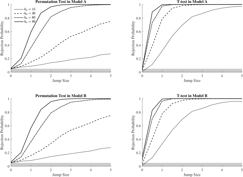
Overall, we find that the permutation test controls size remarkably well under the null hypothesis. Although it appears to be less powerful than the t-test, it does not suffer from the latter’s size distortion which can be severe in the two-factor volatility model. Our results suggest that, given its robustness, the permutation test is a useful complement to the conventional test based on spot estimation and asymptotic Gaussian approximation.
4 An empirical illustration
We apply the proposed permutation test to a recent sample of high-frequency price and volume observations of the S&P 500 ETF (NYSE: SPY) as an empirical illustration. The sampling frequency is one minute; the data source is the TAQ database. With the permutation test, we are interested in testing distributional discontinuities of the ETF’s return, trading volume, and two measures of illiquidity for several FOMC announcements during the COVID-19 pandemic. This setting highlights one of the key merits of the proposed test, namely, it is applicable for a broad variety of high-frequency observations modeled in distinct ways. This is in sharp contrast to the conventional t-test based on (8), which is designed specifically for testing volatility jumps and whose validity relies on the assumption of Brownian shocks. We construct the high-frequency volume series as the total number of shares within each one-minute trading session. The illiquidity measures of interest include Amihud’s measure defined as the ratio between absolute return and dollar trading volume (Amihud (2002)) and the bid-ask spread averaged within each one-minute trading session.
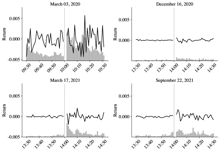
We focus on four important FOMC announcements in the 2020–2021 sample period that are related to distinct aspects of the Federal Reserve’s monetary policy during the COVID-19 pandemic. The first is the announcement made on March 3, 2020, which was also the first FOMC announcement after COVID-19 hit the United States. The Fed stated its decision to lower the federal funds rate by 1/2 percentage point as its first response to counter the pandemic’s negative impact on the economy. The second event occurred on December 16, 2020. At that time, being concerned with the rising long-term yield, many market participants expected that the Fed might implement the so-called “operation twist” to tame the steepening of the yield curve. But this turned out not to be on the Fed’s agenda, and so, the Fed’s “inaction” may be deemed as a shock relative to the market’s anticipation. The third case pertains to the announcement on March 17, 2021. During the press conference, the Fed Chairman suggested that the central bank would be unlikely to raise the rate in the next 2–3 years, which may be regarded as a forward guidance on the target rate. The final example is the announcement on September 22, 2021, when the Fed officially declared its intention to taper the large-scale asset purchase program.
Figure 2 plots the asset return and trading volume of SPY over one-hour windows centered at these announcement times. For ease of comparison, we plot the return and volume data for the four events on the same scale. These plots immediately reveal the highly distinct market conditions at those times. This highlights the usefulness of adopting a high-frequency event-study research design, which allows us to investigate each event separately, rather than pooling information across different announcements under a likely fragile homogeneity assumption. We also observe several interesting patterns regarding how the market responds to the “lumpy” information embedded in the announcements. We generally see a rise in trading activity after the announcement. The price also tends to fluctuate more in the post-announcement window, although the March 3, 2020 event may be an exception as the market was already quite volatile even before the announcement.
As mentioned above, we implement the permutation test described in Algorithm 1 on the ETF’s returns, trading volume, Amihud’s measure, and bid-ask spread constructed on the one-minute sampling frequency. For ease of interpretation, we consider the non-randomized version of the test described in Remark 2.1. We consider two event windows: minutes or minutes. Recall that each FOMC announcement contains two stages. The first is an immediate release of a short summary on the Federal Reserve’s webpage, which will be further detailed in the Fed Chairman’s opening statement during the first (roughly) 10 minutes of the press conference. The second part is a Q&A session in which the Chairman responds to questions from the media, with the first few generally being more important. Given this setup, the shorter window allows us to focus on the immediate impact of the FOMC statement, whereas the longer window further covers the “more subtle” policy information conveyed to the public during the Q&A session. It is worth noting that the 30-minute event window is also adopted in prior work on the high-frequency identification of monetary policy shocks; see Nakamura and Steinsson (2018a).
| Date () | Return | Volume | Amihud | Spread | Return | Volume | Amihud | Spread |
| 03/03/2020 | *** | * | *** | *** | *** | |||
| 12/16/2020 | ** | *** | ** | *** | ** | *** | *** | |
| 03/17/2021 | * | *** | *** | ** | *** | *** | ||
| 09/22/2021 | ** | *** | *** | *** | *** | *** | ||
| Note: The permutation test is implemented following Algorithm 1. For ease of interpretation, we consider the non-randomized version as described in Remark 2.1 using 100,000 i.i.d. permutations. Rejections at the 10%, 5%, and 1% significance levels are indicated by *, **, and ***, respectively. | ||||||||
Table 2 reports the results of the permutation test. Recall that the permutation test applied to asset returns may be interpreted as a test for volatility jumps, as explained in Example 1 (with Brownian shocks) or Example 2 (with more general Lévy shocks).161616Prior work on volatility jumps (see, e.g., Bollerslev et al. (2018) and Li et al. (2021)) focuses exclusively on the case in which volatility is the scaling factor of Brownian shocks. Our permutation test is related to the prior work, but is valid under a more general notion of volatility with respect to non-Brownian shocks. At a significance level of 10%, the permutation test rejects the null of continuity for all events except the one on March 3, 2020. The latter non-rejection is consistent with our previous observation that the volatility of SPY was high even before the announcement. Meanwhile, the test also strongly rejects the null hypothesis of distributional continuity for the volume series, echoing the burst of trading activity seen in Figure 2.
The permutation test applied to the two illiquidity measures generates mixed results. We find some moderate evidence for the distributional discontinuity of Amihud’s measure shortly after the March 3 and December 16 announcements in 2020. For the case with a 30-minute window, we do not reject the null of continuity for any of the announcements. The overall evidence suggests that the FOMC announcements under study did not lead to an abrupt change in the market impact coefficient gauged by Amihud’s measure. Needless to say, this finding per se does not imply that the liquidity condition is unchanged after the announcement, as the notion of liquidity is a multifaceted concept. Indeed, we see that the permutation test applied to the bid-ask spread always strongly rejects the null of continuity. The post-announcement spread tends to be larger than its pre-announcement level, suggesting that it is significantly more costly to trade during the post-announcement trading session.
All in all, the empirical illustration above demonstrates how the proposed permutation test may be used to test for distributional discontinuities for a variety of market variables. This type of versatility is not easily attained by existing methods in the high-frequency econometrics literature. We also see that interesting empirical findings may be obtained even with a small number of observations, which confirms the practical relevance of allowing the window to be possibly fixed in our asymptotic theory for the permutation test.
5 Concluding remarks
In this paper, we propose using a permutation test to detect discontinuities in an economic model at a cutoff point. Relative to the existing literature, we show that the permutation test is well suited for event studies based on time-series data. While nonparametric t-tests have been widely used for this purpose in various empirical contexts, the permutation test proposed in this paper provides a distinct alternative. Instead of relying on asymptotic (mixed) Gaussianity from central limit theorems, we exploit finite-sample properties of the permutation test in the approximating, or “coupling”, two-sample problem.
We demonstrate that our new theory is broadly useful in a wide range of problems in the infill asymptotic time-series setting, which justifies using the permutation test to detect jumps in economic variables such as volatility, trading activity, and liquidity. Compared with the conventional nonparametric t-test, the proposed permutation test has several distinct features. First, the permutation test provides asymptotic size control regardless of whether the sizes of the local subsamples are fixed or growing to infinity. In the latter case, we also establish that the permutation test is consistent. Second, the permutation test is versatile, as it can be applied without modification to many different contexts and under relatively weak conditions.
Appendix: Proofs
Throughout the proofs, we use to denote a positive constant that may change from line to line, and write to emphasize its dependence on some parameter . For any event , we identify it with the associated indicator random variable.
Proof of Theorem 2.1.
Step 1. Define in the same way as but with replaced by . In this step, we show that
| (11) |
Let be defined in the same way as , but with replaced by , as defined in Assumption 2.1(iii). Since and have the same (conditional) distribution,
| (12) |
Let be the event where the ordered values of and correspond to the same permutation of . Since the test statistic is only a function of the rank of the observations, we have in restriction to . Hence,
| (13) |
By (12) and (13), (11) follows from , which will be proved below.
Let for every , and note that . Recall the elementary fact that if a sequence of random variables , then there exists a real sequence such that . Under Assumption 2.1(iii), by applying this result to , we can find a sequence such that
| (14) |
We then observe that
Therefore,
which, together with (14), implies that
| (15) |
Next, consider the following argument:
| (16) |
where the last line holds by Assumption 2.1(ii). By (16) and the bounded convergence theorem,
| (17) |
Step 2. We now prove the assertions in parts (a) and (b) of the theorem. In view of (11), we only need to prove and in these two parts, respectively. For part (a), note that are conditionally i.i.d. and so permutations constitute a group of transformations that satisfy the randomization hypothesis in Lehmann and Romano (2005, Definition 15.2.1). Then, Lehmann and Romano (2005, Theorem 15.2.1) implies that , and then follows from the law of iterated expectations.
To prove part (b), we need some additional notation. To emphasize the dependence of , , and on the original data , we explicitly write them as , , and . With this notation, we can rewrite , since it is computed in the same way as but with replaced by .
We first analyze the asymptotic behavior of . Define the empirical analogue of as
Since the variables are -conditionally i.i.d.,
By Markov’s inequality and the law of iterated expectations, this implies that for each . This and a classical Glivenko–Cantelli theorem (e.g., Davidson (1994, Theorem 21.5)) imply that
| (18) |
By definition,
In addition, we define
Note that the functions and are uniformly bounded. Hence, by the triangle inequality and (18),
| (19) |
Conditional on , the bounded random functions and can be treated as deterministic functions. Next, note that
| (20) |
where the first equality holds by a law of large numbers for the conditionally i.i.d. variables for , and the second equality holds by the definition of . By combining (19) and (20), we deduce that
| (21) |
In turn, by (21) and the condition in part (b), we conclude that
| (22) |
Next, we analyze the asymptotic behavior of . It is useful to consider the following representation of this variable. We denote , where is a random permutation of , independent from the data, and is drawn uniformly from the set of all permutations of . By definition, is the quantile of , conditional on the sample, where the randomness comes from the random realization of . To analyze the permutation distribution, we construct an additional coupling sequence of following the method of Chung and Romano (2013, Section 5.3). We note that their coupling construction does not require the null hypothesis to hold, and it is thus suitable for our current purposes. The result of their coupling construction is another random sequence such that (i) for all in some random subset ; (ii) the cardinality of , denoted , satisfies ; and (iii) are -conditionally i.i.d. with marginal distribution .
For any fixed arbitrary permutation and for , define
By repeatedly using the triangle inequality,
| (23) |
where the last inequality uses the fact that if , and so the summation on the previous line only has bounded terms that can be different from zero; and the statement follows from , , and Markov’s inequality.
For any fixed arbitrary permutation , is the Cramér-von Mises statistic for the -conditionally i.i.d. variables . Hence, by a similar argument leading to (22), we have . By combining this with (23), it follows that
| (24) |
Since this result holds for any arbitrary fixed permutation , it also holds for any pair of permutations considered at random from the set of all possible permutations of , independently from the data. By elementary properties of stochastic convergence, this implies the so-called Hoeffding’s condition (e.g., Lehmann and Romano (2005, Equation (15.10))). By this and Lehmann and Romano (2005, Theorem 15.2.3), the permutation distribution associated with the test statistic , conditional on the data, converges to zero in probability. As a corollary of this,
| (25) |
Proof of Theorem 2.2.
(a) We prove the assertion of part (a) by applying Theorem 2.1(a). We construct the coupling variable as follows:
| (26) |
We set . By Assumption 2.2, are i.i.d. and independent of . Since is -measurable, the variables are -conditionally i.i.d. This verifies the condition in part (a) of Theorem 2.1, which also implies Assumption 2.1(i). It remains to verify conditions (ii) and (iii) in Assumption 2.1.
By a standard localization argument (see Jacod and Protter (2012, Section 4.4.1)), we can strengthen Assumption 2.3 by assuming , , and for some fixed compact set and constant . In particular, takes values in the compact set . By Assumption 2.2, it is then easy to see that the -conditional probability density of is uniformly bounded (and it does not depend on ). This implies condition (ii) of Assumption 2.1.
Finally, we verify condition (iii) of Assumption 2.1. By Assumption 2.2(i), for each , is independent of . Since and are -measurable, we deduce from Assumption 2.3(i) that
| (27) |
Note that under the null hypothesis with , the processes and are identical. Hence, by Assumption 2.3(ii) and (27),
By the maximal inequality under the norm (see, e.g., van der Vaart and Wellner (1996, Lemma 2.2.2)), we further deduce that
| (28) |
Recall that by assumption. Hence,
| (29) |
Note that, by the definitions in (4) and (26),
| (30) |
Combining (29), (30), and Assumption 2.3(iii), we deduce that , which verifies Assumption 2.1(iii). We have now verified all the conditions needed in Theorem 2.1(a), which proves the assertion of part (a) of Theorem 2.2.
(b) We prove the assertion of part (b) by applying Theorem 2.1(b). Under the maintained alternative hypothesis, we have for some constant . The coupling variable now takes the following form
| (31) |
Under Assumption 2.2, it is easy to see that, for each , the variables are -conditionally i.i.d., which verifies Assumption 2.1(i).
We now turn to the remaining conditions in Assumption 2.1. As in part (a), we can invoke the standard localization procedure and assume that the process takes value in a compact set . Note that
where the statement follows from the fact that the process is càdlàg and . Therefore, by enlarging the compact set slightly if necessary, we also have with probability approaching 1. Then, we can verify Assumption 2.1(ii) following the same argument as in part (a). The verification of Assumption 2.1(iii) is also similar.
Finally, we verify the condition in Theorem 2.1(b) pertaining to the conditional CDFs. Note that
It is then easy to see that
Since takes values in the compact set , Assumption 2.2(iii) implies that the lower bound in the above display is bounded away from zero. Hence, for any real sequence . We have now verified all conditions for Theorem 2.1(b), which proves the assertion of part (b) of Theorem 2.2.
Proof of Theorem 2.3.
This proof follows from similar arguments to those used to prove Theorem 2.1. For the sake of brevity, we focus on the only substantial difference, which is how we establish that . Recall that denotes the event where the ordered values of and correspond to the same permutation of . In the case of this proof, this result follows from
where the first inequality follows from and the convergence follows from the assumption that uniformly in .
Proof of Theorem 2.4.
(a) We prove this assertion by applying Theorem 2.3(a). We shall verify the conditions in Theorem 2.3 for , , and . By assumption, the variables are i.i.d. and independent of . Hence, the variables are -conditionally i.i.d.
It remains to verify that uniformly in . By repeating the localization argument used in the proof of Theorem 2.2, we can strengthen Assumption 2.4 with without loss of generality. In particular, takes values in some compact subset . Note that for each , is independent of . By Assumption 2.4(i), we thus have . Then, by Assumption 2.4(ii), we further have . The condition then follows from . By Theorem 2.3(a), we have as asserted.
(b) We prove this assertion by applying Theorem 2.3(b). We verify the conditions in Theorem 2.3 for , , and
Following the same argument as in part (a), we see that are -conditionally i.i.d. for each , and uniformly in . Assumption 2.2(iii) also ensures that for any real sequence . By Theorem 2.3(b), we have that , as asserted.
Supplement: Extension to other test statistics
As explained in Remark 2.2, our main results extend beyond the Cramér-von Mises statistic in (1). We characterize the relevant class of test statistics by the following high-level assumption.
Assumption 5.1.
, where is a sequence of functions that satisfies the following conditions:
(a) is a rank statistic, i.e., for any and with for all , .
(b) For any and , with .
Assumption 5.1 is satisfied for a large class of test statistics, which includes the Cramér-von Mises and Kolmogorov-Smirnov statistics. In fact, the proof of Theorem 2.1 shows that the Cramér-von Mises statistic satisfies Assumption 5.1, and an analogous argument can be used to extend this to the Kolmogorov-Smirnov statistic. We now briefly describe the assumption. Assumption 5.1(a) is an essential ingredient to our methodology. In turn, Assumption 5.1(b) is a mild regularity condition that limits the influence that a few sample observations can have on the test statistic, and is only required to establish our consistency result.
The result proves Theorem 2.1 for any test statistic that satisfies Assumption 5.1. Since Theorem 2.1 is the key to all of the results in the paper, this effectively implies that our findings extend to the class of statistics characterized by Assumption 5.1, as claimed in Remark 2.2.
Theorem 5.1.
(a) If the variables have the same -conditional distribution, we have .
(b) Let denote the test statistic but applied to instead of . If and for any real sequence , we have .
Proof.
This proof follows closely that of Theorem 2.1, which has two steps. Step 1 remains unchanged, as it only relies on Assumption 2.1 and the fact that is a rank statistic, imposed in Assumption 5.1(a). Part (a) of Step 2 also remains unchanged, as it is entirely based on Step 1. To complete this proof, it then suffices to cover the analog of part (b) of Step 2.
We begin by considering the asymptotic behavior of , i.e., the quantile of , conditional on the sample, where the randomness comes from the realization of . As in the proof of Theorem 2.1, we rely on the coupling construction based on Chung and Romano (2013, Section 5.3), which produces a random sequence such that (i) for all in some random subset ; (ii) satisfies ; and (iii) are -conditionally i.i.d. Then, for any fixed arbitrary permutation ,
| (32) |
where the second equality relies on and Assumption 5.1(b), and the last equality relies on , , and Markov’s inequality. We can then repeat the arguments in the proof of Theorem 2.1 to conclude that for any fixed arbitrary permutation . By this with (32), we conclude that . Since was arbitrarily chosen, it then follows that
| (33) |
References
- Amihud (2002) Amihud, Y. (2002): “Illiquidity and Stock Returns: Cross-Section and Time-Series Effects,” Journal of Financial Markets, 5, 31–56.
- Andersen (1996) Andersen, T. G. (1996): “Return Volatility and Trading Volume: An Information Flow Interpretation of Stochastic Volatility,” Journal of Finance, 51, 169–204.
- Andrews (1993) Andrews, D. W. K. (1993): “Tests for Parameter Instability and Structural Change With Unknown Change Point,” Econometrica, 61, 821–856.
- Antoch and Hušková (2001) Antoch, J. and M. Hušková (2001): “Permutation tests in change point analysis,” Statistics & Probability Letters, 53, 273–291.
- Bai and Perron (1998) Bai, J. and P. Perron (1998): “Estimating and Testing Linear Models with Multiple Structural Changes,” Econometrica, 66, 47–78.
- Barndorff-Nielsen and Shephard (2001) Barndorff-Nielsen, O. and N. Shephard (2001): “Non-Gaussian Ornstein–Uhlenbeck-Based Models and some of Their Uses in Financial Economics,” Journal of the Royal Statistical Society, Series B, 63, 167–241.
- Barndorff-Nielsen and Shephard (2006) Barndorff-Nielsen, O. E. and N. Shephard (2006): “Econometrics of Testing for Jumps in Financial Economics Using Bipower Variation,” Journal of Financial Econometrics, 4, 1–30.
- Bollerslev et al. (2018) Bollerslev, T., J. Li, and Y. Xue (2018): “Volume, Volatility, and Public News Announcements,” Review of Economic Studies, 85, 2005–2041.
- Bollerslev and Todorov (2011) Bollerslev, T. and V. Todorov (2011): “Estimation of Jump Tails,” Econometrica, 79, 1727–1783.
- Bugni and Canay (2021) Bugni, F. A. and I. A. Canay (2021): “Testing Continuity of a Density via g-order statistics in the Regression Discontinuity Design,” Journal of Econometrics, 221, 138–159.
- Calonico et al. (2014) Calonico, S., M. D. Cattaneo, and R. Titiunik (2014): “Robust Nonparametric Confidence Intervals for Regression-Discontinuity Designs,” Econometrica, 82, 2295–2326.
- Canay and Kamat (2017) Canay, I. A. and V. Kamat (2017): “Approximate Permutation Tests and Induced Order Statistics in the Regression Discontinuity Design,” The Review of Economic Studies, 85, 1577–1608.
- Cattaneo et al. (2015) Cattaneo, M. D., B. R. Frandsen, and R. Titiunik (2015): “Randomization inference in the regression discontinuity design: An application to party advantages in the US Senate,” Journal of Causal Inference, 3, 1 – 24.
- Cattaneo et al. (2017) Cattaneo, M. D., R. Titiunik, and G. Vazquez-Bare (2017): “Comparing inference approaches for RD designs: A reexamination of the effect of Head Start on child mortality,” Journal of Policy Analysis and Management, 36, 643–681.
- Chernozhukov et al. (2018) Chernozhukov, V., K. Wuthrich, and Y. Zhu (2018): “Exact and Robust Conformal Inference Methods for Predictive Machine Learning With Dependent Data,” Tech. rep., arXiv:1802.06300v3.
- Chow (1960) Chow, G. C. (1960): “Tests of Equality Between Sets of Coefficients in Two Linear Regressions,” Econometrica, 28, 591–605.
- Chung and Romano (2013) Chung, E. and J. P. Romano (2013): “Exact and Asymptotically Robust Permutation Tests,” Annals of Statistics, 41, 484–507.
- Cochrane and Piazzesi (2002) Cochrane, J. H. and M. Piazzesi (2002): “The Fed and Interest Rates - A High-Frequency Identification,” American Economic Review, 92, 90–95.
- Comte and Renault (1998) Comte, F. and E. Renault (1998): “Long Memory in Continuous Time Stochastic Volatility Models,” Mathematical Finance, 8, 291–323.
- Davidson (1994) Davidson, J. (1994): Stochastic Limit Theory, Oxford University Press.
- DiCiccio and Romano (2017) DiCiccio, C. J. and J. P. Romano (2017): “Robust Permutation Tests for Correlation and Regression Coefficients,” Journal of the American Statistical Association, 112, 1211–1220.
- Foster and Nelson (1996) Foster, D. P. and D. B. Nelson (1996): “Continuous Record Asymptotics for Rolling Sample Variance Estimators,” Econometrica, 64, 139–174.
- Hahn et al. (2001) Hahn, J., P. Todd, and W. V. der Klaauw (2001): “Identification and Estimation of Treatment Effects with a Regression-Discontinuity Design,” Econometrica, 69, 201–209.
- Hoeffding (1952) Hoeffding, W. (1952): “The Large-Sample Power of Tests Based on Permutations of Observations,” Annals of Mathematical Statistics, 3, 169–192.
- Horváth and Rice (2014) Horváth, L. and G. Rice (2014): “Extensions of some classical methods in change point analysis,” Test, 23, 219–255.
- Hušková (2004) Hušková, M. (2004): “Permutation principle and bootstrap in change point analysis,” Fields Institute Communications, 44, 273–291.
- Imbens and Kalyanaraman (2011) Imbens, G. and K. Kalyanaraman (2011): “Optimal Bandwidth Choice for the Regression Discontinuity Estimator,” The Review of Economic Studies, 79, 933–959.
- Imbens and Lemieux (2008) Imbens, G. W. and T. Lemieux (2008): “Regression Discontinuity Designs: A Guide to Practice,” Journal of Econometrics, 142, 615 – 635.
- Jacod and Protter (2012) Jacod, J. and P. Protter (2012): Discretization of Processes, Springer.
- Jentsch and Pauly (2015) Jentsch, C. and M. Pauly (2015): “Testing equality of spectral densities using randomization techniques,” Bernoulli, 21, 697–739.
- Kirch (2007) Kirch, C. (2007): “Block permutation principles for the change analysis of dependent data,” Journal of Statistical Planning and Inference, 137, 2453–2474.
- Kirch and Steinebach (2006) Kirch, C. and J. Steinebach (2006): “Permutation principles for the change analysis of stochastic processes under strong invariance,” Journal of Computational and Applied Mathematics, 186, 68–88.
- Lee and Lemieux (2010) Lee, D. S. and T. Lemieux (2010): “Regression Discontinuity Designs in Economics,” Journal of Economic Literature, 48, 281–355.
- Lehmann and Romano (2005) Lehmann, E. L. and J. P. Romano (2005): Testing Statistical Hypothesis, Springer.
- Li and Liu (2020) Li, J. and Y. Liu (2020): “Efficient Estimation of Integrated Volatility Functionals under General Volatility Dynamics,” Econometric Theory, Forthcoming.
- Li et al. (2017) Li, J., V. Todorov, and G. Tauchen (2017): “Jump Regressions,” Econometrica, 85, 173–195.
- Li et al. (2021) Li, J., V. Todorov, and Q. Zhang (2021): “Testing the Dimensionality of Policy Shocks,” Review of Economics and Statistics, forthcoming.
- Li and Xiu (2016) Li, J. and D. Xiu (2016): “Generalized Method of Integrated Moments for High-frequency Data,” Econometrica, 84, 1613–1633.
- Nakamura and Steinsson (2018a) Nakamura, E. and J. Steinsson (2018a): “High-Frequency Identification of Monetary Non-Neutrality: The Information Effect,” Quarterly Journal of Economics, 133, 1283–1330.
- Nakamura and Steinsson (2018b) ——— (2018b): “Identification in Macroeconomics,” Journal of Economic Perspectives, 32, 59–86.
- Stock (1994) Stock, J. (1994): “Chapter 46 Unit Roots, Structural Breaks and Trends,” Elsevier, vol. 4 of Handbook of Econometrics, 2739 – 2841.
- Thistlethwaite and Campbell (1960) Thistlethwaite, D. L. and D. T. Campbell (1960): “Regression-discontinuity Analysis: An alternative to the Ex Post Facto Experiment.” Journal of Educational Psychology, 51, 309–317.
- Todorov and Tauchen (2012) Todorov, V. and G. Tauchen (2012): “Realized Laplace Transforms for Pure-jump Semimartingales,” The Annals of Statistics, 40, 1233–1262.
- van der Vaart and Wellner (1996) van der Vaart, A. and J. Wellner (1996): Weak Convergence and Empirical Processes, Springer-Verlag.