Periodically-driven quantum thermal machines from warming up to limit cycle
Abstract
Theoretical treatments of periodically-driven quantum thermal machines (PD-QTMs) are largely focused on the limit-cycle stage of operation characterized by a periodic state of the system. Yet, this regime is not immediately accessible for experimental verification. Here, we present a general thermodynamic framework that can handle the performance of PD-QTMs both before and during the limit-cycle stage of operation. It is achieved by observing that periodicity may break down at the ensemble average level, even in the limit-cycle phase. With this observation, and using conventional thermodynamic expressions for work and heat, we find that a complete description of the first law of thermodynamics for PD-QTMs requires a new contribution, which vanishes only in the limit-cycle phase under rather weak system-bath couplings. Significantly, this contribution is substantial at strong couplings even at limit cycle, thus largely affecting the behavior of the thermodynamic efficiency. We demonstrate our framework by simulating a quantum Otto engine building upon a driven resonant level model. Our results provide new insights towards a complete description of PD-QTMs, from turn-on to the limit-cycle stage and, particularly, shed light on the development of quantum thermodynamics at strong coupling.
Introduction.– A tantalizing goal of quantum thermodynamics is to investigate, analyze and ultimately design thermal machines on the quantum scale Scovil and Schulz-DuBois (1959); Geva and Kosloff (1992); Gemmer et al. (2009); Seifert (2012); Pekola (2015); Kosloff (2013); Goold et al. (2016); Vinjanampathy and Anders (2016); Benenti et al. (2017); Binder et al. (2018); Seifert (2019). Among the various routes towards this vision, devising periodically-driven quantum thermal machines (PD-QTMs) in which work can be extracted through externally driving a quantum working substance represents a paradigmatic one. This field has attracted much attention in recent years with intriguing theoretical proposals Brandner et al. (2015); Brandner and Seifert (2016); Proesmans et al. (2016); Newman et al. (2017); Alecce et al. (2015); Perarnau-Llobet et al. (2018); Mohammady and Romito (2019); Kloc et al. (2019); Pezzutto et al. (2019); Mohammady and Romito (2019); Park et al. (2019); Solfanelli et al. (2020); akmak and Altintas (2020); Wiedmann et al. (2020); Shirai et al. (2021); Strasberg et al. (2021) together with delicate experimental realizations in various platforms Abah et al. (2012); Roßnagel et al. (2014); Dechant et al. (2015); Krishnamurthy et al. (2016); Ro nagel et al. (2016); Peterson et al. (2019); Klatzow et al. (2019); de Assis et al. (2019); Pekola and Khaymovich (2019); von Lindenfels et al. (2019).
Existing theories on PD-QTMs are largely carried out in the limit-cycle stage of operation, where the working substance should recoil to its original state after a driving cycle (see, e.g., Refs.Feldmann and Kosloff (2004); Brandner et al. (2015); Brandner and Seifert (2016); Insinga et al. (2016); Proesmans et al. (2016); Insinga et al. (2018); Mohammady and Romito (2019); Shirai et al. (2021); Menczel and Brandner (2019)). Although the limit-cycle regime enables theoretical simplicity, it faces potential challenges. On the one hand, recent studies have pointed out that the state of the working substance needs not inherit the periodicity of external drivings at finite times Menczel and Brandner (2019); Pezzutto et al. (2019); Wiedmann et al. (2020), namely, there may exist a transient warming-up phase for the operation of PD-QTMs before a limit cycle sets in. On the other hand, the limit-cycle stage is not immediately accessible experimentally, which may lead to discrepancy between theoretical predictions and experimental measurements. Addressing these challenges requires a unified thermodynamic description of both the warming-up and limit-cycle phases of PD-QTMs, which is, however, still missing.
In this work, we present a thermodynamic framework that deals with cycle-number dependent thermodynamic quantities. As such, it allows us to characterize in a unified manner the performance of PD-QTMs in both the warming-up and limit-cycle phases. Our theory relies on the observation that periodicity can break down at the ensemble average level, namely, with being a periodic observable and the driving period. This breakdown is trivial in the transient warming-up phase where even the state of the working substance does not behave in a periodic manner. However, nontrivially, this breakdown can show up in the limit-cycle phase if involves bath degrees of freedom, a scenario which is frequently encountered in studies of quantum thermodynamics (see recent discussions Talkner and Hänggi (2020); Seshadri and Galperin (2021) and reference therein).
Building upon this observation, we find that the thermodynamic characterization of PD-QTMs generally acquires a new contribution in both the warming-up and limit-cycle phases, besides the conventional notions of work and heat. Particularly, through completing the first law of thermodynamics [cf. Eq. (4)] and ensuring its validity across the whole parameter space at all times, we identify this extra term (denoted as hereafter) as the change of an ensemble average within a cycle [cf. Eq. (5)]; denotes the Hamiltonian for the working substance (system-bath coupling). Intriguingly, this term vanishes only in the limit-cycle phase provided that the system-bath coupling is rather weak. We further uncover that contributions from the term play a nontrivial role in shaping behavior of the thermodynamic efficiency [cf. Eq. (6)] in both the warming-up and limit-cycle phases, especially at strong coupling, compared with existing characterizations, which largely neglect it.
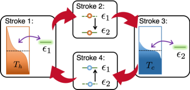
We illustrate our general framework using the quantum Otto heat engine (see Fig. 1 for a sketch), with a driven resonant electronic level as the working substance.
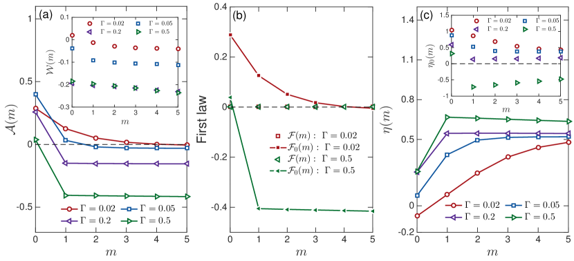
Based on simulations, we confirm our theoretical predictions of the behaviors of thermodynamic quantities incorporating the term, including the first law of thermodynamics and the efficiency (see Fig. 2). In comparison, conventional definitions without fail to capture the correct thermodynamics, especially at strong coupling where the term is substantial in both warm-up and limit-cycle regimes. The framework presented here allows the description of PD-QTMs even before the limit cycle stage, and at strong coupling, both aspects crucial for describing experimental systems and advancing the field of quantum thermodynamics.
Quantum thermodynamics of generic PD-QTMs.– Generally, PD-QTMs can be modeled as (, hereafter)
| (1) |
Here, denotes a semiclassically-driven working substance with the understanding that the working substance exchanges work with an external agent which we do not explicitly include within the quantum description. consists of a hot (h) and a cold (c) thermal bath and denotes a time-dependent system-bath coupling. Here, is a time-dependent coefficient describing the contact switching of the reservoir, used to implement thermodynamic strokes (see, e.g., Refs. Wiedmann et al. (2020); Pancotti et al. (2020); Shirai et al. (2021)). We assume periodic protocols such that with the period of the driving.
To analyze the quantum thermodynamics of the PD-QTM, we introduce the definitions of heat and work based on the complete Hamiltonian dynamics, Bruch et al. (2016); Oz et al. (2020); Wiedmann et al. (2020); Cangemi et al. (2021). This approach naturally avoids the problem of the partitioning of the system-bath interaction. Denoting by the total density matrix of the composite system, the integrated injected work and absorbed heat from the bath during the -th cycle with a non-negative integer are uniquely defined as Bruch et al. (2016); Oz et al. (2020); Wiedmann et al. (2020); Cangemi et al. (2021)
| (2) | |||||
| (3) |
Here, for an arbitrary operator , the trace is performed over system and bath degrees of freedom. The introduction of the cycle-number () dependent thermodynamic quantities allows us to characterize the performance of PD-QTMs in both the warming-up and limit-cycle stages. Note that the expression for absorbed heat is consistent with the definition employed in quantum transport scenarios Esposito et al. (2015a, b); Bergmann and Galperin (2021). For the work definition, it naturally incorporates work costs for implementing a time-dependent system-bath coupling Newman et al. (2017). In our convention, a heat engine corresponds to , and .
Since the integrand in Eq. (2) is just with the internal energy of the composite system, we can express Eq. (2) as . This immediately leads to an intriguing observation: , generally valid since for a PD-QTM. Note that this difference does not prevent the existence of a limit-cycle phase for the reduced system density matrix , Feldmann and Kosloff (2004); Brandner et al. (2015); Brandner and Seifert (2016); Insinga et al. (2016); Proesmans et al. (2016); Insinga et al. (2018); Mohammady and Romito (2019); Shirai et al. (2021); Menczel and Brandner (2019), since the bath state needs not be a periodic function at all. This simple observation has a profound consequence: An operator involving bath degrees of freedom generally shows , even when . Namely, the periodicity can break down at the ensemble average level.
We now turn to the first law of thermodynamics for PD-QTMs. In terms of our definitions for heat and work, it takes the following exact form 111One can obtain the present first law by combining the expression with the Hamiltonian decomposition of Eq. (1).,
| (4) |
Crucially, besides the conventional notions of work and heat, an extra quantity appears, ,
| (5) |
Here, we denote by . In arriving at the first law Eq. (4), we emphasize that no approximations were invoked. The term reflects the change to after a cycle, highlighting the nontrivial role of the system-bath coupling in quantum engines Shirai et al. (2021); Talkner and Hänggi (2020). In the warming-up phase where even the system density matrix does not inherit the periodicity of the driving protocol, one naturally expects a nonzero . In the limit-cycle phase, vanishes only when the system-bath coupling is negligible compared to the system energy scale since then . Otherwise, at strong coupling, we still have as [see discussion before Eq. (4)]. This result contradicts previous studies (see, e.g., Ref. Wiedmann et al. (2020)), which neglected the contribution from regardless of system-bath coupling strength. This first law and the nontrivial behavior of represent our first main result. As for the second law of thermodynamics, we still observe the conventional Clausius inequality Esposito et al. (2010); Brandner and Seifert (2016); Seshadri and Galperin (2021), with the von Neumann entropy of the working substance.
Using Eq. (4), the averaged thermodynamic efficiency over a cycle, , reads
| (6) |
Here, is the common definition of efficiency Alecce et al. (2015); Mohammady and Romito (2019); Park et al. (2019); Solfanelli et al. (2020); akmak and Altintas (2020), which has been applied to strong coupling scenarios Perarnau-Llobet et al. (2018); Wiedmann et al. (2020). Intriguingly, gains an additional contribution , compared to . we point out that Eq. (6) is completely general as no assumptions were invoked in its derivation: It can be applied to arbitrary PD-QTMs in both the warming-up and limit-cycle phases, regardless of the system-bath coupling strength. On the contrary, can only be applied to the weak-coupling scenario in the limit-cycle phase where vanishes [see discussion below Eq. (5)]. This working definition for the efficiency is our second main result.
Example: Driven resonant level engine.– To substantiate and exemplify our main results [cf. Eqs. (4), (5) and (6)] we present a numerical example of a quantum Otto heat engine (see Fig. 1) that extracts work from heat baths with a resonant level model Ludovico et al. (2014); Esposito et al. (2015a, b); Ochoa et al. (2016); Bruch et al. (2016); Thingna et al. (2017); Dou et al. (2018); Oz et al. (2019); Dou et al. (2020); Oz et al. (2020),
| (7) |
Here, the working substance consists of a single spinless electronic level with the annihilation operator and time-dependent energy . The dot is alternating its coupling to two fermionic baths (leads) of different temperatures. annihilates an electron with energy in the -lead that couples to the central level with as the tunneling rate. The -lead is occupied according to the Fermi-Dirac distribution with an inverse temperature and a chemical potential ; for our purpose, we set and . The coupling of the central level to the leads is given by the spectral densities . In what follows, we consider the wideband limit such that and adopt symmetric couplings, . The time-dependent coefficients equal when the coupling to the -lead is turned on and otherwise, thus enabling thermalization strokes in the Otto cycle.
The complete Otto cycle with period consists of four strokes; see Fig. 1 for an illustration: (1) Stroke 1 (): In this isochoric thermalization step, the central level with a fixed energy is coupled to the hot lead. (2) Stroke 2 (): The energy of the isolated central level is shifted from to . (3) Stroke 3 (): In this isochoric thermalization step, the central level with a fixed energy is coupled to the cold lead. (4) Stroke 4 (): The energy of the isolated central level is tuned back from to . We remark that the adopted cycle protocol does not enforce a periodicity on the system density matrix a priori as we just tune the energy of the central level. The engine needs a transient warming-up process before settling into a limit-cycle operation mode. Moreover, we do not enforce an adiabatic work-extracting process, namely, strokes 2 and 4 can span finite times. In fact, the amount of work generated during strokes 2 and 4 is independent of the detailed functional form of connecting fixed end points as the charge occupation of the central level during these two strokes remains fixed; in Ref. SM , we exploit this fact together with an equilibrium charge occupation expression Liu and Segal (2020) (note that we attach the central level to two leads alternatively in the Otto cycle) to estimate the heat-engine operation regime and determine relevant values of to be used in simulations.
The cycle number-dependent thermodynamics is simulated by employing the driven Liouville von-Neumann equation method Ajisaka et al. (2012); Zelovich et al. (2014); Chen et al. (2014); Zelovich et al. (2017); Chiang and Hsu (2020) whose performance for addressing quantum thermodynamics up to strong coupling has been carefully assessed Oz et al. (2019, 2020); we relegate simulation details, including numerical implementation, initial condition at and adopted parameter values, to SM . A typical set of thermodynamic results is depicted in Fig. 2. Quantities at are evaluated for the first cycle .
The behavior of along with the work is presented in Fig. 2 (a); results for the heat exchange can be found in SM . We find that as the coupling strength increases, the magnitude of becomes more pronounced. From this it is evident that based on our heat and work definitions, the complete first law of thermodynamics at all times should read as depicted in Fig. 2 (b). In contrast, the sum considered in other studies (see, e.g., Refs. Mohammady and Romito (2019); Wiedmann et al. (2020)) approaches zero only in the weak-coupling scenario, and in the limit-cycle stage (see red line for in Fig. 2 (b) at where the engine is reaching the limit-cycle phase; this is confirmed in SM with a long-time simulation for ). Importantly, beyond the weak coupling regime, the faulty first law that neglects the term deviates from zero at all times. Perhaps most surprisingly, Fig. 2 (c) reveals that if one adopts the incomplete definition of efficiency, i.e. Eq. (6) without , at strong coupling one would predict no heat engine behavior in this regime (see inset of Fig. 2 (c)). However, by properly including the contribution, thus accounting for the effect of system-bath coupling, we find that the system does operate as a heat engine, consistent with the negative injected work value reported in the inset of Fig. 2 (a).
Besides the aforementioned basic features that reinforce the validity of our general theory, there are a few points worth discussing further: (i) Weak coupling scenarios need more transient cycles to warm up than the strong coupling counterparts before a limit-cycle phase sets in. Comparing the behaviors of and as a function of , we argue that the former can assess the number of transient cycles based on its magnitude variation with increasing . For instance, from Fig. 2 (a), we observe that an engine of requires at least 4 transient cycles; note is the number of completed cycles. In contrast, an engine with needs just one cycle to warm up. We have verified that the number of transient cycles is independent of the initial charge occupation of the central level. (ii) The thermodynamic efficiency does not reach a stationary value at strong couplings with increasing (see curve for in Fig. 2 (c)), noting that the heat depends on the state of the bath, which needs not be a periodic function; see SM for the behavior of while varying and the coupling strength. This finding implies that a characterization based on a single cycle in the limit-cycle phase may not be applicable at strong couplings. (iii) In our simulations, increases as the coupling strength increases. This seems at odds with some studies Perarnau-Llobet et al. (2018); Newman et al. (2020), which have observed the opposite trend. However, we point out that these studies used the incomplete definition . Indeed, the inset of Fig. 2 (c) shows that decreases as increases, until it becomes invalid for very large coupling strength. This suggests that interactions with the baths are in fact helpful in the heat-work conversion process Shirai et al. (2021). The dramatic qualitative difference between the conventional definition and the correct expression demonstrates why it is crucial to adopt the complete expressions, including the term.
Discussion.– One may argue that the term [cf. Eq. (5)] can be absorbed by redefining heat and work (see discussions in Refs. Bruch et al. (2016); Ochoa et al. (2016); Dou et al. (2018)). We would like to point out that (i) the work definition we adopted [cf. Eq. (2)] already comprises the internal energy change of the total composite system, and (ii) introducing an effective bath Hamiltonian with the replacement Bruch et al. (2016); Ochoa et al. (2016); Dou et al. (2018) and accordingly modifying the heat definition [cf. Eq. (3)], one is still not able to eliminate the term, by comparing the definitions Eq. (3) and (5). After all, as we argued, the term originates from the fact that periodicity breaks down at the ensemble average level even in the limit-cycle phase.
Recognizing the generic presence of , it is tempting to explore whether the inclusion of work costs for the attachment and detachment of the working substance to and from the baths can affect the behavior of . While here we switched between strokes by tuning [see Eq. (Periodically-driven quantum thermal machines from warming up to limit cycle)] using a sharp step function alternating between and , one could adopt a smooth function. We leave this point to future investigations.
Although our thermodynamic framework is applicable to general PD-QTMs, a direct measurement of is experimentally challenging since it requires measuring energy change associated with the system-bath coupling. However, the utility of our framework is that it provides predictions for efficiency as a function of the cycle number, enabling a direct comparison with experiments. Exploring feasible measurement schemes for quantifying the role of , in light of recent experimental advances in single-electron and superconducting circuits Pekola (2015); Pekola and Khaymovich (2019), is an interesting future direction.
In summary, we have presented a unified, consistent thermodynamic theory, with cycle-number dependent thermodynamic quantities, which describes the operation of PD-QTMs both before and during the limit-cycle phase, covering strongly-coupled thermal machines. The unearthed term (i) provides a complete description of the first law of thermodynamics and (ii) substantially modifies the efficiency of the engine, particularly at strong coupling, compared with existing characterizations. With its ability to describe PT-QTMs from the warming up phase to their limit cycle and from weak to strong coupling, we expect this framework to promote the experimental development of quantum thermal machines.
Acknowledgement.– J.L. and D.S. acknowledge support from the Natural Sciences and Engineering Research Council (NSERC) of Canada Discovery Grant and the Canada Research Chairs Program.
References
- Scovil and Schulz-DuBois (1959) H. E. D. Scovil and E. O. Schulz-DuBois, “Three-level masers as heat engines,” Phys. Rev. Lett. 2, 262 (1959).
- Geva and Kosloff (1992) E. Geva and R. Kosloff, “On the classical limit of quantum thermodynamics in finite time,” J. Chem. Phys. 97, 4398 (1992).
- Gemmer et al. (2009) J. Gemmer, M. Michel, and G. Mahler, Quantum Thermodynamics (Springer-Verlag, Berlin, 2009).
- Seifert (2012) U. Seifert, “Stochastic thermodynamics, fluctuation theorems and molecular machines,” Rep. Prog. Phys. 75, 126001 (2012).
- Pekola (2015) J. P. Pekola, “Towards quantum thermodynamics in electronic circuits,” Nat. Phys. 11, 118 (2015).
- Kosloff (2013) R. Kosloff, “Quantum thermodynamics: A dynamical viewpoint,” Entropy 15, 2100 (2013).
- Goold et al. (2016) J. Goold, M. Huber, A. Riera, L. del Rio, and P. Skrzypczyk, “The role of quantum information in thermodynamics?a topical review,” J. Phys. A: Math. Theor. 49, 143001 (2016).
- Vinjanampathy and Anders (2016) S. Vinjanampathy and J. Anders, “Quantum thermodynamics,” Contemp. Phys. 57, 545 (2016).
- Benenti et al. (2017) G. Benenti, G. Casati, K. Saito, and R. S. Whitney, “Fundamental aspects of steady-state conversion of heat to work at the nanoscale,” Phys. Rep. 694, 1 (2017).
- Binder et al. (2018) F. Binder, L. A. Correa, C. Gogolin, J. Anders, and G. Adesso, Thermodynamics in the Quantum Regime (Springer International, 2018).
- Seifert (2019) U. Seifert, “From stochastic thermodynamics to thermodynamic inference,” Annu. Rev. Condens. Matter Phys. 10, 171 (2019).
- Brandner et al. (2015) K. Brandner, K. Saito, and U. Seifert, “Thermodynamics of micro- and nano-systems driven by periodic temperature variations,” Phys. Rev. X 5, 031019 (2015).
- Brandner and Seifert (2016) K. Brandner and U. Seifert, “Periodic thermodynamics of open quantum systems,” Phys. Rev. E 93, 062134 (2016).
- Proesmans et al. (2016) K. Proesmans, Y. Dreher, M. Gavrilov, J. Bechhoefer, and C. Van den Broeck, “Brownian duet: A novel tale of thermodynamic efficiency,” Phys. Rev. X 6, 041010 (2016).
- Newman et al. (2017) D. Newman, F. Mintert, and A. Nazir, “Performance of a quantum heat engine at strong reservoir coupling,” Phys. Rev. E 95, 032139 (2017).
- Alecce et al. (2015) A. Alecce, F. Galve, N. Lo Gullo, L. Dell’Anna, F. Plastina, and R. Zambrini, “Quantum otto cycle with inner friction: finite-time and disorder effects,” New J. Phys. 17, 075007 (2015).
- Perarnau-Llobet et al. (2018) M. Perarnau-Llobet, H. Wilming, A. Riera, R. Gallego, and J. Eisert, “Strong coupling corrections in quantum thermodynamics,” Phys. Rev. Lett. 120, 120602 (2018).
- Mohammady and Romito (2019) M. H. Mohammady and A. Romito, “Efficiency of a cyclic quantum heat engine with finite-size baths,” Phys. Rev. E 100, 012122 (2019).
- Kloc et al. (2019) M. Kloc, P. Cejnar, and G. Schaller, “Collective performance of a finite-time quantum otto cycle,” Phys. Rev. E 100, 042126 (2019).
- Pezzutto et al. (2019) M. Pezzutto, M. Paternostro, and Y. Omar, “An out-of-equilibrium non-markovian quantum heat engine,” Quantum Sci. Technol. 4, 025002 (2019).
- Park et al. (2019) J-M. Park, S. Lee, H-M. Chun, and J. D. Noh, “Quantum mechanical bound for efficiency of quantum otto heat engine,” Phys. Rev. E 100, 012148 (2019).
- Solfanelli et al. (2020) A. Solfanelli, M. Falsetti, and M. Campisi, “Nonadiabatic single-qubit quantum otto engine,” Phys. Rev. B 101, 054513 (2020).
- akmak and Altintas (2020) S. akmak and F. Altintas, “Quantum carnot cycle with inner friction,” Quantum Inf. Processing 19, 248 (2020).
- Wiedmann et al. (2020) M. Wiedmann, J. T. Stockburger, and J. Ankerhold, “Non-markovian dynamics of a quantum heat engine: out-of-equilibrium operation and thermal coupling control,” New J. Phys. 22, 033007 (2020).
- Shirai et al. (2021) Y. Shirai, K. Hashimoto, R. Tezuka, C. Uchiyama, and N. Hatano, “Non-markovian effect on quantum otto engine: Role of system-reservoir interaction,” Phys. Rev. Research 3, 023078 (2021).
- Strasberg et al. (2021) P. Strasberg, C. W. Wächtler, and G. Schaller, “Autonomous implementation of thermodynamic cycles at the nanoscale,” Phys. Rev. Lett. 126, 180605 (2021).
- Abah et al. (2012) O. Abah, J. Roßnagel, G. Jacob, S. Deffner, F. Schmidt-Kaler, K. Singer, and E. Lutz, “Single-ion heat engine at maximum power,” Phys. Rev. Lett. 109, 203006 (2012).
- Roßnagel et al. (2014) J. Roßnagel, O. Abah, F. Schmidt-Kaler, K. Singer, and E. Lutz, “Nanoscale heat engine beyond the carnot limit,” Phys. Rev. Lett. 112, 030602 (2014).
- Dechant et al. (2015) A. Dechant, N. Kiesel, and E. Lutz, “All-optical nanomechanical heat engine,” Phys. Rev. Lett. 114, 183602 (2015).
- Krishnamurthy et al. (2016) S. Krishnamurthy, S. Ghosh, D. Chatterji, R. Ganapathy, and A. K. Sood, “A micrometre-sized heat engine operating between bacterial reservoirs,” Nat. Phys. 12, 1134 (2016).
- Ro nagel et al. (2016) J. Ro nagel, Samuel T. Dawkins, K. N. Tolazzi, O. Abah, E. Lutz, F. Schmidt-Kaler, and K. Singer, “A single-atom heat engine,” Science 352, 325 (2016).
- Peterson et al. (2019) J. P. S. Peterson, T. B. Batalhão, M. Herrera, A. M. Souza, R. S. Sarthour, I. S. Oliveira, and R. M. Serra, “Experimental characterization of a spin quantum heat engine,” Phys. Rev. Lett. 123, 240601 (2019).
- Klatzow et al. (2019) J. Klatzow, J. N. Becker, P. M. Ledingham, C. Weinzetl, K. T. Kaczmarek, D. J. Saunders, J. Nunn, I. A. Walmsley, R. Uzdin, and E. Poem, “Experimental demonstration of quantum effects in the operation of microscopic heat engines,” Phys. Rev. Lett. 122, 110601 (2019).
- de Assis et al. (2019) R. J. de Assis, T. M. de Mendonça, C. J. Villas-Boas, A. M. de Souza, R. S. Sarthour, I. S. Oliveira, and N. G. de Almeida, “Efficiency of a quantum otto heat engine operating under a reservoir at effective negative temperatures,” Phys. Rev. Lett. 122, 240602 (2019).
- Pekola and Khaymovich (2019) J. P. Pekola and I. M. Khaymovich, “Thermodynamics in single-electron circuits and superconducting qubits,” Annu. Rev. Condens. Matter Phys. 10, 193 (2019).
- von Lindenfels et al. (2019) D. von Lindenfels, O. Gräb, C. T. Schmiegelow, V. Kaushal, J. Schulz, Mark T. Mitchison, John Goold, F. Schmidt-Kaler, and U. G. Poschinger, “Spin heat engine coupled to a harmonic-oscillator flywheel,” Phys. Rev. Lett. 123, 080602 (2019).
- Feldmann and Kosloff (2004) T. Feldmann and R. Kosloff, “Characteristics of the limit cycle of a reciprocating quantum heat engine,” Phys. Rev. E 70, 046110 (2004).
- Insinga et al. (2016) A. Insinga, B. Andresen, and P. Salamon, “Thermodynamical analysis of a quantum heat engine based on harmonic oscillators,” Phys. Rev. E 94, 012119 (2016).
- Insinga et al. (2018) A. Insinga, B. Andresen, P. Salamon, and R. Kosloff, “Quantum heat engines: Limit cycles and exceptional points,” Phys. Rev. E 97, 062153 (2018).
- Menczel and Brandner (2019) P. Menczel and K. Brandner, “Limit cycles in periodically driven open quantum systems,” J. Phys. A: Math. Theor. 52, 43LT01 (2019).
- Talkner and Hänggi (2020) P. Talkner and P. Hänggi, “Colloquium: Statistical mechanics and thermodynamics at strong coupling: Quantum and classical,” Rev. Mod. Phys. 92, 041002 (2020).
- Seshadri and Galperin (2021) N. Seshadri and M. Galperin, “Entropy and information flow in quantum systems strongly coupled to baths,” Phys. Rev. B 103, 085415 (2021).
- Pancotti et al. (2020) N. Pancotti, M. Scandi, M. T. Mitchison, and M. Perarnau-Llobet, “Speed-ups to isothermality: Enhanced quantum thermal machines through control of the system-bath coupling,” Phys. Rev. X 10, 031015 (2020).
- Bruch et al. (2016) A. Bruch, M. Thomas, S. Viola Kusminskiy, F. von Oppen, and A. Nitzan, “Quantum thermodynamics of the driven resonant level model,” Phys. Rev. B 93, 115318 (2016).
- Oz et al. (2020) A. Oz, O. Hod, and A. Nitzan, “Numerical approach to nonequilibrium quantum thermodynamics: Nonperturbative treatment of the driven resonant level model based on the driven liouville von-neumann formalism,” J. Chem. Theory Comput. 16, 1232 (2020).
- Cangemi et al. (2021) L. M. Cangemi, M. Carrega, A. De Candia, V. Cataudella, G. De Filippis, M. Sassetti, and G. Benenti, “Optimal energy conversion through antiadiabatic driving breaking time-reversal symmetry,” Phys. Rev. Research 3, 013237 (2021).
- Esposito et al. (2015a) M. Esposito, M. A. Ochoa, and M. Galperin, “Quantum thermodynamics: A nonequilibrium green’s function approach,” Phys. Rev. Lett. 114, 080602 (2015a).
- Esposito et al. (2015b) M. Esposito, M. A. Ochoa, and M. Galperin, “Nature of heat in strongly coupled open quantum systems,” Phys. Rev. B 92, 235440 (2015b).
- Bergmann and Galperin (2021) N. Bergmann and M. Galperin, “A green?s function perspective on the nonequilibrium thermodynamics of open quantum systems strongly coupled to baths,” Eur. Phys. J. Spec. Top. , – (2021).
- Note (1) One can obtain the present first law by combining the expression with the Hamiltonian decomposition of Eq. (1).
- Esposito et al. (2010) M. Esposito, K. Lindenberg, and C. Van den Broeck, “Entropy production as correlation between system and reservoir,” New J. Phys. 12, 013013 (2010).
- Ludovico et al. (2014) M. Ludovico, J. Lim, M. Moskalets, L. Arrachea, and D. Sánchez, “Dynamical energy transfer in ac-driven quantum systems,” Phys. Rev. B 89, 161306 (2014).
- Ochoa et al. (2016) M. A. Ochoa, A. Bruch, and A. Nitzan, “Energy distribution and local fluctuations in strongly coupled open quantum systems: The extended resonant level model,” Phys. Rev. B 94, 035420 (2016).
- Thingna et al. (2017) J. Thingna, F. Barra, and M. Esposito, “Kinetics and thermodynamics of a driven open quantum system,” Phys. Rev. E 96, 052132 (2017).
- Dou et al. (2018) W. Dou, M. A. Ochoa, A. Nitzan, and J. Subotnik, “Universal approach to quantum thermodynamics in the strong coupling regime,” Phys. Rev. B 98, 134306 (2018).
- Oz et al. (2019) I. Oz, O. Hod, and A. Nitzan, “Evaluation of dynamical properties of open quantum systems using the driven liouville-von neumann approach: methodological considerations,” Mol. Phys. 117, 2083 (2019).
- Dou et al. (2020) W. Dou, J. Bätge, A. Levy, and M. Thoss, “Universal approach to quantum thermodynamics of strongly coupled systems under nonequilibrium conditions and external driving,” Phys. Rev. B 101, 184304 (2020).
- (58) See Supplemental Material for the estimation of heat-engine operation regime for the driven resonant level model, simulation details regarding the driven Liouville von-Neumann method and additional simulation results.
- Liu and Segal (2020) J. Liu and D. Segal, “Sharp negative differential resistance from vibrational mode softening in molecular junctions,” Nano Lett. 20, 6128 (2020).
- Ajisaka et al. (2012) S. Ajisaka, F. Barra, C. Mejía-Monasterio, and T. Prosen, “Nonequlibrium particle and energy currents in quantum chains connected to mesoscopic fermi reservoirs,” Phys. Rev. B 86, 125111 (2012).
- Zelovich et al. (2014) T. Zelovich, L. Kronik, and O. Hod, “State representation approach for atomistic time-dependent transport calculations in molecular junctions,” J. Chem. Theory Comput. 10, 2927 (2014).
- Chen et al. (2014) L. Chen, T. Hansen, and I. Franco, “Simple and accurate method for time-dependent transport along nanoscale junctions,” J. Phys. Chem. C 118, 20009 (2014).
- Zelovich et al. (2017) T. Zelovich, T. Hansen, Z. Liu, J. B. Neaton, L. Kronik, and O. Hod, “Parameter-free driven liouville-von neumann approach for time-dependent electronic transport simulations in open quantum systems,” J. Chem. Phys. 146, 092331 (2017).
- Chiang and Hsu (2020) T-M. Chiang and L-Y. Hsu, “Quantum transport with electronic relaxation in electrodes: Landauer-type formulas derived from the driven liouville?von neumann approach,” J. Chem. Phys. 153, 044103 (2020).
- Newman et al. (2020) D. Newman, F. Mintert, and A. Nazir, “Quantum limit to nonequilibrium heat-engine performance imposed by strong system-reservoir coupling,” Phys. Rev. E 101, 052129 (2020).
Supplemental material: Periodically-driven quantum thermal machines from warming up to limit cycle
In this supplemental material, we first identify the parameter regime where the driven resonant level model operates as a quantum Otto heat engine. Next, we provide simulation details regarding the numerical implementation of the driven Liouville von-Neumann (DLvN) approach. We also present additional simulation results that complement those included in the main text.
I I. Regime of heat engine behavior of the driven resonant level model
Here we determine the operation regime of a quantum Otto heat engine made of a driven resonant level model from a general perspective. We rely on the facts that (i) only strokes 2 and 4 of a quantum Otto cycle produce nonzero work and (ii) that the charge occupation of the central level remains unaltered during these two strokes. We assume here that the engine has reached the limit-cycle phase at , starting from the remote past , such that we can resort to the integrated injected work obtained within a cycle to access the sign of work,
| (S1) | |||||
Here, . Since remains fixed during strokes 2 and 4, we simplify the above expression as
| (S2) | |||||
Here, denote the occupation after the hot (cold) isochore. We have used the fact that , , which stems from the definition of our quantum Otto cycle (see Fig. 1 of the main text).
Since we can set the time intervals long enough to allow complete equilibration, can be estimated using their equilibrium expressions (see, e.g., Ref. Liu and Segal (2020))
| (S3) |
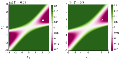
Here, we considered symmetric coupling with , is the Fermi-Dirac distribution of the -lead characterized by an inverse temperature and a chemical potential . By combining Eqs. (S2) and (I), we determine the operation regimes of a heat engine, i.e. for which parameters the work per cycle, in the limit cycle region is negative, . Fig. S1 depicts a set of calculation results while varying for two different coupling strengths ; heat engine operation regimes with negative are highlighted by the red zones. For simulation purposes, throughout this study we choose the values and as marked by white crosses in the figure.
II II. Driven Liouville von-Neumann approach
We employ the so-called driven Liouville von-Neumann (DLvN) approach Oz et al. (2019, 2020); Chiang and Hsu (2020) to simulate the dynamics of the driven resonant level model. Since the total Hamiltonian of the driven resonant level model is quadratic, all observables can be constructed from the correlator with . The average is evaluated with respect to the total initial state. For simplicity, we denote hereafter. To calculate the dynamics of thermodynamic observables, we introduce the following matrix
| (S4) |
Here, stands for the dot population, are diagonal blocks of leads, and are the dot-lead coherences vectors. Correspondingly, the total Hamiltonian matrix is expressed as
| (S5) |
Here, are diagonal blocks of lead level energies, , which are taken to be equally spaced over the bandwidth in numerical simulations. are column vectors containing tunneling elements . With the above definitions, the driven Liouville von-Neumann (DLvN) equation governing the evolution of takes the following form Oz et al. (2019, 2020); Chiang and Hsu (2020)
| (S6) |
Here, the equilibrium correlator elements are . The lead driving rate constant is set to be of the order of the lead energy spacing. It represents the timescale on which thermal relaxation takes place in the leads due to their couplings to an implicit superbath Oz et al. (2019, 2020). We check and show below in Figs. S3-S4 that the dynamics of thermodynamic observables is fairly insensitive to the specific choice of in the coupling range for considered in this study.
A A. Numerical implementation
To simplify the implementation of the DLvN approach, we consider the wideband limit for the leads, such that with determined by with a constant density of state of the -lead Oz et al. (2019, 2020). In numerical treatment, we represent each lead by a single energy band of a finite bandwidth (specifically, electronic levels in the metals extend from to ). We use a finite number, , of equally spaced single-electron states with energy spacing ( accordingly). Note that to get reasonable results, we require that and . The DLvN equation Eq. (S6) is subject to an initial factorized state
| (S7) |
It is then numerically evolved using the fourth-order Runge-Kutta method with a fixed time step . We check the convergence of results with respect to , and (see below Figs. S3-S4 for examples).
B B. Working expressions for thermodynamic observables
In terms of the correlator and Hamiltonian , the work and term can be directly obtained as
| (S8) |
Here, . We also introduced the following matrix forms
| (S12) | |||||
| (S16) |
The heat absorbed by the resonant level from the bath should be evaluated as
| (S17) |
where the reservoir matrices read
| (S21) | |||||
| (S25) |
and the second term on the right-hand-side of Eq. (3) denotes the heat current exchange between the -lead and its implicit bath (see Eq. (59) of Ref. Oz et al. (2020)) with
| (S29) | |||||
| (S33) |
Using the DLvN equation (S6) and noting that and , we readily check that the first law of thermodynamics,
| (S34) |
is satisfied by the above expressions.
III III. Driving protocol and convergence check
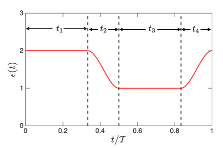
To facilitate detailed numerical simulations, we need to specify the functional form of . The overall work output within a cycle is independent of the detailed form of , as we explained in Sec. I. Therefore, we have the freedom to choose its functional form with the understanding that it should be at least once differentiable (since is needed so as to determine the amount of generated work during a cycle) and . Specifically, we adopt the following protocol for within a period (see Fig. S2):
| (S35) |
where , and .
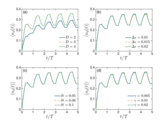
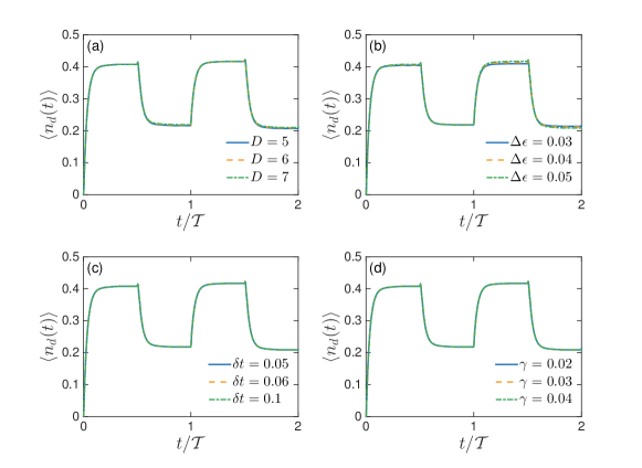
Using the above driving protocol [cf, Eq. (S35)] within the DLvN equation [cf, Eq. (S6)], we readily check the convergence of various quantities with respect to phenomenological damping rate , band width , lead energy spacing and evolution time step . Considering the weak coupling limit, in Fig. S3, we show a typical set of results for charge occupation of the resonant level when varying [panel (a)], [panel (b)], [panel (c)] and [panel (d)]. Analogous simulations are presented in Fig. S4, using .
We summarize in Table I parameter sets used in the present study, which lead to well-converged results.
| 3 | 3 | 5 | 6 | |
| 0.006 | 0.015 | 0.0125 | 0.03 | |
| 0.1 | 0.1 | 0.1 | 0.1 | |
| 0.006 | 0.015 | 0.0125 | 0.03 |
IV IV. Additional simulation results
Here we present thermodynamic results that complement the results in the main text.
A A. Heat
In Fig. S5, we present results for heat exchange with increasing cycle number .
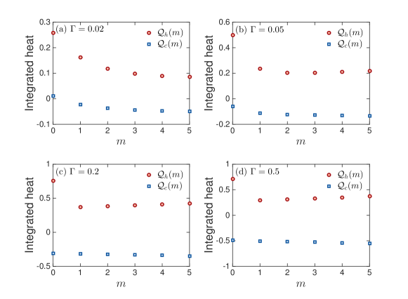
Two points are to be highlighted, illustrating the important aspects of the present study, namely that periodicity can break down at the ensemble average level and the presence of term is a necessity:
(i) In the limit-cycle phase as marked by stationary term (see discussion in the main text regarding this point), the heats still vary as the cycle number increases. This phenomenon is particularly clear at strong couplings (see Fig. S5 (c) (d)). Since heat is defined as the change of the bath (lead) energy within a cycle, it thus depends only on the lead density matrix. One can therefore infer that the lead density matrix needs not inherit the periodicity of the system density matrix, as argued in the main text. (ii) At large coupling strength, we observe that (Fig. S5 (d)). We remark that this seemingly unphysical result is allowed by the first law of thermodynamics as this imbalance is precisely compensated by a negative term (see Fig. 2 (b) of the main text).
B B. Long-time behavior at weak coupling
In Fig. S6, we illustrate the long-time behavior for a weak-coupling scenario, .
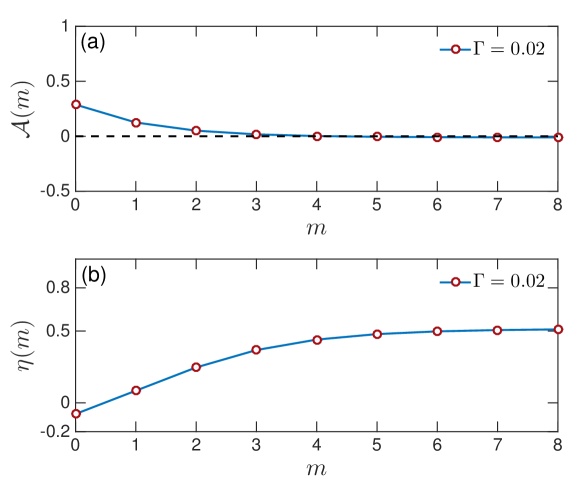
From the figure, we confirm that the system indeed reaches its limit-cycle phase at , as argued in the main text.