Performance Analysis of Coded OTFS Systems over High-Mobility Channels

Without loss of generality, we consider a coded OTFS system as shown in Fig. 1. Let $M$ be the number of sub-carriers and $N$ be the number of time slots for each OTFS symbol, respectively. An information sequence $\bf{u}$ is channel-encoded and then modulated into ${\bf{x}}\in{{\mathbb{A}}^{MN}}$ with length $MN$. Let us arrange ${\bf{x}}$ into a 2D matrix ${\bf{X}}\in{{\mathbb{A}}^{M\times N}}$, i.e., ${\bf{x}}\buildrel\Delta\over{=}\textrm{vec}\left({\bf{X}}\right)$, representing the symbols in the DD domain, whose $(k,l)$-th element $x\left[{k,l}\right]$ is the modulated signal in the $k$-th Doppler and $l$-th delay grid [6], for $0\leq k\leq N-1,0\leq l\leq M-1$. Each transmitted symbol in the TF domain $X\left[{n,m}\right],0\leq n\leq N-1,0\leq m\leq M-1$, is then obtained based on ${\bf{X}}$ via the inverse symplectic fast Fourier transform (ISFFT) as follows [6]

A brief diagram regarding the DD and TF domain transformation is shown in Fig. 2, where $\Delta f$ is the frequency spacing between adjacent sub-carriers and $T={1\mathord{\left/{\vphantom{1{\Delta f}}}\right.\kern-1.2pt}{\Delta f}}$ is the corresponding TF domain time slot duraion. Therefore, each OTFS system takes the total bandwidth of $M\Delta f$ and symbol duration $NT$. In particular, the sampling time $1/(M\Delta T)$ and sampling frequency $1/(NT)$ are referred to as the delay resolution and the Doppler resolution of the DD grid, respectively [10], which indicate how precise the acquisition of the channel delay and Doppler can be for the underlying OTFS system. After the domain transformation (ISFFT), the TF domain transmitted symbol $X\left[{n,m}\right]$ is then modulated via a conventional OFDM modulator. The time domain OTFS signal $s\left(t\right)$ is written as

where the $g_{{\rm{tx}}}(t)$ denotes the pulse shaping filter. As described above, for OFDM-based OTFS implementation, the OTFS modulator can be viewed as a concatenation of a precoder (ISFFT) and a conventional OFDM modulator [11], where the OFDM modulator consists of an inverse FFT (IFFT) block and a pulse shaping filter $g_{{\rm{tx}}}(t)$. Similar to [6], we consider the DD domain representation of the time-varying channel, where the channel impulse response is given by

In (3), $P$ is the number of independent resolvable paths while $h_{i}$, $\tau_{i}$, and $\nu_{i}$ are the channel coefficients, delay shifts, and Doppler shifts corresponding to the $i$-th path, respectively. Let $\bar{w}\left(t\right)$ be the additive white Gaussian noise process with one-sided power spectral density (PSD) $N_{0}$. The received signal can be written as

Let $g_{{\rm{rx}}}(t)$ be the filter adopted at the receiver side. The received symbols $Y\left[{n,m}\right]$ in the TF domain are then obtained by

Substituting (4) into (5) and after similar manipulations as in [10], (5) can be simplified as

where $\bar{w}\left[{n,m}\right]$ is the corresponding TF domain noise sample and ${H_{n,m}}\left[{n^{\prime},m^{\prime}}\right]$ is the TF domain channel response, given by

In (7), the function ${A_{{g_{{\rm{tx}}}},{g_{{\rm{rx}}}}}}\left({{\tau_{\Delta}},{\nu_{\Delta}}}\right)$ is the so-called cross-ambiguity function, which indicates the interference level between the TF domain symbols due to the channel dispersion and is given by [10]

Hence, the received symbols $y\left[{k,l}\right]$ in the DD domain are obtained by performing the SFFT on the TF domain received symbols $Y\left[{n,m}\right]$ which are written as

where $w\left[{k,l}\right]$ denotes the equivalent AWGN samples in the DD domain. In specific, the DD domain received symbols $y\left[{k,l}\right]$ can be arranged into the 2D received symbol matrix ${\bf{Y}}$ according to the DD grid, whose $(k,l)$-th element is $y\left[{k,l}\right]$. For the ease of presentation and analysis, we consider the vector form representation of the input-output relationship of OTFS system in the DD domain based on (9) in the sequel.

Let ${\bf{x}}\buildrel\Delta\over{=}\textrm{vec}\left({\bf{X}}\right)\in{{\mathbb{A}}^{MN}}$ and ${\bf{y}}\buildrel\Delta\over{=}\textrm{vec}\left({\bf{Y}}\right)\in{{\mathbb{A}}^{MN}}$ denote the vector forms of the transmitted symbols ${\bf{X}}$ and the received symbols ${\bf{Y}}$ in the DD domain, respectively. According to (9), we have

where $\bf{w}$ is the corresponding noise vector and ${{\bf{H}}_{{\rm{eff}}}}$ of size $MN\times MN$ is the effective channel matrix in the DD domain. Assuming that both $g_{{\rm{tx}}}(t)$ and $g_{{\rm{rx}}}(t)$ are rectangular pulses, with a reduced CP frame format, the effective channel matrix ${{\bf{H}}_{{\rm{eff}}}}$ is given by [20]

where ${\bm{\Pi}}$ is the permutation matrix (forward cyclic shift), i.e.,

and ${\bm{\Delta}}=\textrm{diag}\{z^{0},z^{1},...,z^{MN-1}\}$ is a diagonal matrix with $z\buildrel\Delta\over{=}{e^{\frac{{j2\pi}}{{MN}}}}$ [20]. In (11), $l_{i}$ and $k_{i}$ are the delay and Doppler indices corresponding to the $i$-th path, respectively, and we have

Note that the term $-{1\mathord{\left/{\vphantom{12}}\right.\kern-1.2pt}2}\leq{\kappa_{i}}\leq{1\mathord{\left/{\vphantom{12}}\right.\kern-1.2pt}2}$ denotes the fractional Doppler which corresponds to the fractional shift from the nearest Doppler [10]. On the other hand, since the typical value of the sampling time ${1\mathord{\left/{\vphantom{1{M\Delta f}}}\right.\kern-1.2pt}{M\Delta f}}$ is in the delay domain usually sufficiently small, the impact of fractional delays in typical wide-band systems can be neglected [8]. It should be noted that (11) still holds even for the fractional Doppler case, i.e., ${\kappa_{i}}\neq 0$, due to the properties of diagonal matrix $\bm{\Delta}$. For simplicity, we only consider the integer Doppler case in this paper. To facilitate the following analysis, we assume that the delay and Doppler indices $l_{i}$ and $k_{i}$ follow the discrete uniform distribution. In specific, we have $l_{i}\in\left[{0,{l_{\max}}}\right]$, where $l_{\max}$ is the maximum delay index. We also have $k_{i}\in\left[{-{k_{\max}},{k_{\max}}}\right]$, where $k_{\max}$ is the maximum Doppler index¹¹1The maximum Doppler shift is given by ${\nu_{\max}}=\frac{v}{c}{f_{c}}$, where $v$ is the relative user equipment (UE) speed, $c$ is the speed of light, and $f_{c}$ is the carrier frequency, respectively. Thus, the maximum Doppler index is given by ${k_{\max}}={\nu_{\max}}NT$ [10]. The maximum delay shift is given by ${\tau_{\max}}=\frac{d_{\rm{max}}}{c}$, where $d_{\rm{max}}$ is the maximum distance among the $P$ channel paths.. In particular, let ${{\bm{\omega}}_{\tau}}$ and ${{\bm{\omega}}_{\nu}}$ denote the vectors of delay indices and Doppler indices, respectively, i.e., ${{\bm{\omega}}_{\tau}}=\left[{{l_{1}},{l_{2}},\ldots,{l_{P}}}\right]^{\rm{T}}$, ${{\bm{\omega}}_{\nu}}=\left[{{k_{1}},{k_{2}},\ldots,{k_{P}}}\right]^{\rm{T}}$, respectively. Therefore, according to [13], (10) can be rewritten as

where ${\bf{\Phi}}_{{{\bm{\omega}}_{\tau}},{{\bm{\omega}}_{\nu}}}\left({\bf{x}}\right)$ is referred to as the equivalent codeword matrix and it is a concatenated matrix of size $MN\times P$ constructed by the column vector ${{\bf{\Xi}}_{i}}{\bf{x}}$ , i.e.,

and ${{\bf{\Xi}}_{i}}$ is given by

In (14), $\bf{h}$ is the path coefficient vector of size $P\times 1$, i.e., ${\bf{h}}={\left[{{h_{1}},{h_{2}},...,{h_{P}}}\right]^{\rm{T}}}$, where the elements in ${\bf{h}}$ are assumed to be independent and identically distributed complex Gaussian random variables. Besides, we assume that $h_{i}$ has the mean $\mu$ and the variance $1/(2P)$ per real dimension²²2Here, we assume a uniform power delay profile of the channel., for $1\leq i\leq P$. In particular, we note that if $\mu=0$, $\left|{{h_{i}}}\right|$ follows the Rayleigh distribution, which will be considered as a special case in our error performance analysis and code design. Based on (14), the error performance analysis of the OTFS systems will be conducted in the next section.

Notice that $\bf{h}$, ${{\bm{\omega}}_{\tau}}$, and ${{{\bm{\omega}}_{\nu}}}$ are independent from each other. Therefore, the unconditional PEP can be derived by firstly averaging (20) over ${|{{{\tilde{h}}_{i}}}|}$ term by term which results in

Furthermore, we consider a special case where ${{K_{i}}}=0$ and ${\small|{{{\tilde{h}}_{i}}}\small|}$ follows the Rayleigh distribution, i.e., ${\small|{{{h}_{i}}}\small|}$ also follows the Rayleigh distribution. In the case of Rayleigh fading, (22) can be further simplified as

By noticing that the term $\prod\nolimits_{i=1}^{P}{{\lambda_{i}}}$ equals to the determinant of ${\bf{\Omega}}\left({\bf{e}}\right)$, (23) can be written as

It should be noted that (24) is consistent with the analysis in [14]. On the other hand, the PEP in (24) depends on the delay and Doppler indices ${\bm{\omega}}_{\tau}$ and ${\bm{\omega}}_{\nu}$. In order to derive the unconditional PEP, we need to find the statistical distribution for the determinant of ${\bf{\Omega}}\left({\bf{e}}\right)$ regarding the delay and Doppler indices. Unfortunately, such a task is generally intractable [19] and is normally handled by applying the Monte Carlo method without providing any important insight. Instead of resorting to the Monte Carlo method, we apply proper bounding techniques to evaluate the determinant of ${\bf{\Omega}}\left({\bf{e}}\right)$ in order to obtain some general results about the unconditional PEP. In particular, we assume that ${\bf{\Omega}}\left({\bf{e}}\right)$ is of full-rank for any channel parameters ${{\bm{\omega}}_{\tau}}$ and ${{{\bm{\omega}}_{\nu}}}$ and error sequence [13, 15], in which case we have the following property.

Property 1 (Gram matrix [22]): Let ${\bar{\bf{u}}_{i}}\buildrel\Delta\over{=}{{\bf{\Xi}}_{i}}{\bf{e}}$, for $1\leq i\leq P$, where ${\bf{\Xi}}_{i}$ is given by (16). Then, $\left\{{{\bar{\bf{u}}_{1}},{\bar{\bf{u}}_{2}},\ldots{\bar{\bf{u}}_{P}}}\right\}$ form a list of independent vectors chosen from the $P$-dimensional complex inner-product subspace $\mathbb{H}^{P}$. Thus, the codeword difference matrix ${\bf{\Omega}}\left({\bf{e}}\right)$ is positive definite Hermitian and it is a Gram matrix corresponding to the vectors $\left\{{{\bar{\bf{{u}}}_{1}},{\bar{\bf{{u}}}_{2}},\ldots{\bar{\bf{{u}}}_{P}}}\right\}$.

Based on the property of ${\bf{\Omega}}\left({\bf{e}}\right)$, we now introduce four important Lemmas, which will be served as the building blocks for our error performance analysis for coded OTFS systems.

Lemma 1 (Main diagonal elements of ${\bf{\Omega}}\left({\bf{e}}\right)$): The main diagonal elements of the codeword difference matrix ${\bf{\Omega}}\left({\bf{e}}\right)$ are of the same value ${d_{\rm{E}}^{2}\left({\bf{e}}\right)}$, where $d_{\rm{E}}^{2}\left({\bf{e}}\right)={{\bf{e}}^{\rm{H}}}{\bf{e}}$ is the squared Euclidean distance for a pair of codewords ${\bf{x}}$ and ${\bf{x^{\prime}}}$ with the corresponding to the error sequence $\bf{e}$.

Proof: By considering (15), the $i$-th diagonal element of ${\bf{\Omega}}\left({\bf{e}}\right)$ is given by ${{\bf{e}}^{\rm{H}}}{\bf{\Xi}}_{i}^{\rm{H}}{{\bf{\Xi}}_{i}}{\bf{e}}$, and it is equal to the inner product of ${{{{\bf{\bar{u}}}}_{i}}}$. Furthermore, we have

where (25) is due to the diagonal properties of ${\bm{\Pi}}$ and $\bm{\Delta}$, respectively, and (26) is due to the property of the Kronecker product. Therefore, the term ${{\bf{e}}^{\rm{H}}}{\bf{\Xi}}_{i}^{\rm{H}}{{\bf{\Xi}}_{i}}{\bf{e}}$ is further simplified as ${d_{\rm{E}}^{2}\left({\bf{e}}\right)}$. This completes the proof of Lemma 1.

Lemma 2 (Trace of ${\bf{\Omega}}\left({\bf{e}}\right)$): The trace of the codeword difference matrix ${\bf{\Omega}}\left({\bf{e}}\right)$ is ${Pd_{\rm{E}}^{2}\left({\bf{e}}\right)}$.

Proof: This lemma is a straightforward extension of Lemma 1.

Lemma 3 (Lower bound on the trace of ${{{\left({{\bf{\Omega}}\left({\bf{e}}\right)}\right)}^{-1}}}$): The trace of the inverse of the codeword difference matrix ${\bf{\Omega}}\left({\bf{e}}\right)$ is lower-bounded by

where the equality holds if ${\bf{\Omega}}\left({\bf{e}}\right)$ is a diagonal matrix, i.e., ${\bf{\Omega}}\left({\bf{e}}\right)=\textrm{diag}\left\{{d_{\rm{E}}^{2}{\left({\bf{e}}\right)},\ldots,d_{\rm{E}}^{2}}{\left({\bf{e}}\right)}\right\}$.

Proof: The proof is given in Appendix A.

Lemma 4 (Lower bound on the summation of eigenvalue squares of ${{{{{\bf{\Omega}}\left({\bf{e}}\right)}}}}$): The summation of the squared eigenvalues of ${{{{{\bf{\Omega}}\left({\bf{e}}\right)}}}}$ is lower-bounded by

where the equality holds if ${\bf{\Omega}}\left({\bf{e}}\right)$ is a diagonal matrix, i.e., ${\bf{\Omega}}\left({\bf{e}}\right)=\textrm{diag}\left\{{d_{\rm{E}}^{2}{\left({\bf{e}}\right)},\ldots,d_{\rm{E}}^{2}}{\left({\bf{e}}\right)}\right\}$.

Proof: It is obvious that the eigenvalues $\lambda_{i}$ of the codeword difference matrix ${{\bf{\Omega}}\left({\bf{e}}\right)}$ are all positive when ${{\bf{\Omega}}\left({\bf{e}}\right)}$ is full-rank. Therefore, we apply the Cauchy-Schwarz inequality and the following holds

where the equality is only achieved when the eigenvalues of ${\bf{\Omega}}\left({\bf{e}}\right)$ are the same, e.g., ${\bf{\Omega}}\left({\bf{e}}\right)=\textrm{diag}\left\{{d_{\rm{E}}^{2}{\left({\bf{e}}\right)},\ldots,d_{\rm{E}}^{2}}{\left({\bf{e}}\right)}\right\}$. This completes the proof of Lemma 4.

The above Lemmas show some important properties of the codeword difference matrix ${\bf{\Omega}}\left({\bf{e}}\right)$. Based on these properties of ${\bf{\Omega}}\left({\bf{e}}\right)$, we can now consider the following lower bounds of the determinant for the codeword difference matrix ${\bf{\Omega}}\left({\bf{e}}\right)$.

Theorem 1 (Lower bound on the determinant of ${\bf{\Omega}}\left({\bf{e}}\right)$): The determinant of the codeword difference matrix ${\bf{\Omega}}\left({\bf{e}}\right)$ is lower-bounded by

where the equality holds if ${\bf{\Omega}}\left({\bf{e}}\right)$ is a diagonal matrix, i.e., ${\bf{\Omega}}\left({\bf{e}}\right)=\textrm{diag}\left\{{d_{\rm{E}}^{2}{\left({\bf{e}}\right)},\ldots,d_{\rm{E}}^{2}}{\left({\bf{e}}\right)}\right\}$.

Proof: The proof is given in Appendix B.

It should be noted that (30) still depends on the channel parameters ${\bm{\omega}}_{\tau}$ and ${\bm{\omega}}_{\nu}$. To obtain an unconditional lower bound, we apply an approximation to the determinant bound which is summarized in the following Theorem.

Theorem 2 (Approximated lower bound on the determinant of ${\bf{\Omega}}\left({\bf{e}}\right)$): The determinant of the codeword difference matrix ${\bf{\Omega}}\left({\bf{e}}\right)$ can be approximately lower-bounded by

where the approximation is exact if ${\bf{\Omega}}\left({\bf{e}}\right)$ is a diagonal matrix, i.e., ${\bf{\Omega}}\left({\bf{e}}\right)=\textrm{diag}\left\{{d_{\rm{E}}^{2}{\left({\bf{e}}\right)},\ldots,d_{\rm{E}}^{2}}{\left({\bf{e}}\right)}\right\}$.

Proof: The proof is given in Appendix C.

Note that the approximated lower bound of the determinant of ${\bf{\Omega}}\left({\bf{e}}\right)$ does not depend on the delay and Doppler indices. Furthermore, based on Theorem 2, it is not hard to notice that the determinant of the codeword difference matrix ${\bf{\Omega}}\left({\bf{e}}\right)$ can be approximated by the term ${\left({d_{\rm{E}}^{2}\left({\bf{e}}\right)}\right)^{P}}$. In particular, the approximation becomes exact if ${\bf{\Omega}}\left({\bf{e}}\right)=\textrm{diag}\left\{{d_{\rm{E}}^{2}{\left({\bf{e}}\right)},\ldots,d_{\rm{E}}^{2}}{\left({\bf{e}}\right)}\right\}$, which can be interpreted as the projections of the error sequence $\bf{e}$ onto each independent resolvable path, i.e., ${\bar{\bf{u}}_{i}}$, are orthogonal to each other. According to Theorem 2, we obtain the unconditional PEP as

Based on (32), we notice that the unconditional PEP for OTFS modulation depends on ${d_{\rm{E}}^{2}\left({\bf{e}}\right)}$ and number of independent resolvable paths $P$. In particular, the term $P$ in the denominator can be interpreted as the energy averaging with respect to the number of independent paths, while the term ${\left({d_{\rm{E}}^{2}\left({\bf{e}}\right)}\right)^{-P}}$ indicates the potential improvement of the error performance introduced by channel coding. Furthermore, according to (32), we refer to the power of the signal-to-noise ratio (SNR) as the diversity gain, which dominates the exponential behaviour of the error performance for OTFS systems against the average SNR. On the other hand, the term ${{d_{\rm{E}}^{2}\left({\bf{e}}\right)}\mathord{\left/{\vphantom{{d_{\rm{E}}^{2}\left({\bf{e}}\right)}P}}\right.\kern-1.2pt}P}$ is referred to as the coding gain, which characterizes the approximate improvement of coded OTFS systems over the uncoded counterpart with the same diversity gain, i.e., the same exponent $-P$ [17]. It is interesting to see from (32) that, there exists a fundamental trade-off between the diversity gain and the coding gain which is formally stated in the following.

Corollary 1 (Trade-off between diversity and coding gain): For a given channel code, the diversity gain of OTFS systems improves with the number of independent resolvable paths $P$, while the coding gain declines.

Based on Corollary 1, we note that when $P$ is small, the diversity gain is small. In this case, the squared Euclidean distance between codewords is crucial for OTFS systems as an optimized code can greatly improve the error performance. On the other hand, when $P$ is large, there is a large diversity gain. In this case, it is expected that the code design can only offer a limited error performance improvement. However, it should also be noted that the coding gain always improves with the increase of $d_{\rm{E}}^{2}\left({\bf{e}}\right)$, regardless of the value of channel parameter $P$ according to (32). Therefore, a preliminary guideline for the code design for the OTFS systems is to maximize the minimum value of $d_{\rm{E}}^{2}\left({\bf{e}}\right)$ among all pairs of codewords of the code.

To verify the accuracy of the derived unconditional PEP bound, we numerically compare the coding gain corresponding to (32) and (24). In particular, recalling (24), after some manipulations, we obtain

Hence, we refer to the term ${{{{\left({\det\left({{\bf{\Omega}}\left({\bf{e}}\right)}\right)}\right)}^{\frac{{\rm{1}}}{P}}}}\mathord{\left/{\vphantom{{{{\left({\det\left({{\bf{\Omega}}\left({\bf{e}}\right)}\right)}\right)}^{\frac{{\rm{1}}}{P}}}}P}}\right.\kern-1.2pt}P}$ as the conditional coding gain of the OTFS systems for given channel parameters ${\bm{\omega}}_{\tau}$ and ${\bm{\omega}}_{\nu}$, as ${{\det\left({{\bf{\Omega}}\left({\bf{e}}\right)}\right)}}$ is a function of ${{{\bm{\omega}}_{\tau}}},{{{\bm{\omega}}_{\nu}}}$. We can also obtain the average coding gain with respect to various channel parameters ${{{\bm{\omega}}_{\tau}}},{{{\bm{\omega}}_{\nu}}}$ and error sequences $\bf{e}$. On the other hand, from the unconditional PEP upper bound (32), we call the function $f\left({d_{\rm{E}}^{2}\left({\bf{e}}\right)}\right)={{d_{\rm{E}}^{2}\left({\bf{e}}\right)}\mathord{\left/{\vphantom{{d_{\rm{E}}^{2}\left({\bf{e}}\right)}P}}\right.\kern-1.2pt}P}$ the coding gain bound of the OTFS systems. Now let us compare the average coding gain and the coding gain obtained from the performance bound via simulations. In particular, we consider a binary phase shift keying (BPSK) signal for the OTFS system with $M=2$ and $N=5$, and error sequences with ${d_{\rm{E}}^{2}\left({\bf{e}}\right)}$, where the maximum delay $l_{\rm{max}}$ and Doppler index $k_{\rm{max}}$ are set to be $2$ and $4$, respectively. To be more specific, we numerically average the conditional coding gains subjected to all error sequences with ${d_{\rm{E}}^{2}\left({\bf{e}}\right)}$ and channel parameters ${{{\bm{\omega}}_{\tau}}},{{{\bm{\omega}}_{\nu}}}$ to obtain the average coding gain.

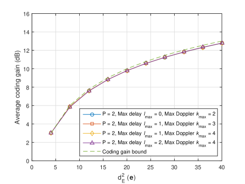
Fig. 3 shows the comparison between the average coding gain and the corresponding coding gain bound in decibels (dB) for $P=2$. As shown in the figure, different values of maximum delay and Doppler indices do not have a strong impact on the average coding gain. Meanwhile, it can be observed in the figure that the average coding gain improves with the increase of the squared Euclidean distance ${d_{\rm{E}}^{2}\left({\bf{e}}\right)}$. Furthermore, the derived coding gain bound shows a close match with the overall average coding gain, especially when ${d_{\rm{E}}^{2}\left({\bf{e}}\right)}$ is small.

Fig. 4 illustrates the average coding gain and the corresponding coding gain bound (in dashed lines) in decibels (dB) with respect to different values of $P$. Without loss of generality, we set the maximum delay index $l_{\rm{max}}$ and the maximum Doppler index $k_{\rm{max}}$ as $2$ and $4$, respectively. As shown in the figure, given ${d_{\rm{E}}^{2}\left({\bf{e}}\right)}$, the average coding gain decreases with the increase of the number of paths $P$, which is consistent with Corollary 1. Similar to the previous figure, the coding gain bounds match well with the general behaviour of average coding gains, especially when $P$ is small, which verifies the correctness of our derivation. On the other hand, we notice that the derived coding gain bound slightly diverge from the average coding gains, when $P$ is large. This observation motivates us to derive a more suitable approximation for the coding gain for large $P$, the details of which will be given in the following subsection.

When there is a large number of independent resolvable paths of the channel, i.e., the value of $P$ is large, the unconditional PEP can be more accurately bounded by considering the strong law of large number [23, 18]. In specific, the term $\sum\limits_{i=1}^{P}{{\lambda_{i}}{{|{{{\tilde{h}}_{i}}}|}^{2}}}$ in (20) approaches a Gaussian random variable, due to the central limit theorem [24].

Notice that ${{\tilde{h}}_{i}}$ follows the complex Gaussian distribution, with mean ${\mu_{{{\tilde{h}}_{i}}}}=\mathbb{E}\left[{\bf{h}}\right]\cdot{{\bf{v}}_{i}}$ and variance $1/(2P)$ per real dimension. Therefore, for the ease of derivation, we normalize the variance and rewrite (20) as

where ${\bar{h}_{i}}=\sqrt{P}{\tilde{h}_{i}}$. Note that $\left\{{{{\bar{h}}_{1}},{{\bar{h}}_{2}},...,{{\bar{h}}_{r}}}\right\}$ are independent complex Gaussian random variables with mean ${\mu_{{{\bar{h}}_{i}}}}={\sqrt{P}}{\mu_{{{\tilde{h}}_{i}}}}$ and variance $1/2$ per real dimension. Furthermore, it is obvious that $\left|{{{\bar{h}}_{i}}}\right|$ follows the Rician distribution with Rician factor ${{\bar{K}}_{i}}={\left|{{\mu_{{{\bar{h}}_{i}}}}}\right|^{2}}$ and a unit variance. Thus, it can be shown that ${{{\left|{{{\bar{h}}_{i}}}\right|}^{2}}}$ follows a noncentral chi-squared distribution with two degrees of freedom (DoFs) and noncentrality parameter $S={{\bar{K}}_{i}}$, whose mean and variance are given by

Next, we derive the unconditional PEP by means of Gaussian approximation. To start with, let $\psi=\sum\limits_{i=1}^{P}{{\lambda_{i}}{{\left|{{{\bar{h}}_{i}}}\right|}^{2}}}$. According to (35) and (36), we approximate $\psi$ as a Gaussian random variable, whose mean is ${\mu_{\psi}}=\sum\limits_{i=1}^{P}{{\lambda_{i}}\left({1+{{{\bar{K}}_{i}}}}\right)}$ and variance is $\sigma_{\psi}^{2}=\sum\limits_{i=1}^{P}{\lambda_{i}^{2}\left({1+2{{\bar{K}}_{i}}}\right)}$. Thus, according to the Gaussian distribution of $\psi$, the conditional PEP in (20) is upper-bounded by

Considering

we obtain

Similar to the previous subsection, we consider the special case of Rayleigh fading.

In the case of Rayleigh fading, i.e., $|{{{\bar{h}}_{i}}}|$ and $|{{h_{i}}}|$ follow the Rayleigh distribution, we have ${\mu_{\psi}}=\sum\limits_{i=1}^{P}{{\lambda_{i}}}$ and $\sigma_{\psi}^{2}=\sum\limits_{i=1}^{P}{\lambda_{i}^{2}}$. Therefore, the right hand side of (39) is given by

Furthermore, we consider the Chernoff bound of the Q-function [23]

and (40) can be further upper-bounded by

when

Based on (42), the unconditional PEP can be approximately upper-bounded as shown in the following Theorem.

Theorem 3 (Unconditional PEP upper bound for large $P$): For a large value of $P$ and a reasonably high SNR, i.e., $\frac{{{E_{s}}}}{{4{N_{0}}}}\geq\frac{P}{{d_{\rm{E}}^{2}\left({\bf{e}}\right)}}$, the unconditional PEP of OTFS systems can be approximately upper-bounded by

Proof: The proof is given in Appendix D.

It should be noted that, for $P\geq 4$, the approximation in Theorem 3 is sufficiently accurate owing to the strong law of the large number [18, 23]. On the other hand, the number of paths $P$ is usually smaller than the squared Euclidean distance $d_{\rm{E}}^{2}\left({\bf{e}}\right)$ for practical wireless transmissions with good channel codes ³³3For example, a popular industry-standard rate-$1/2$ convolutional code with code memory of $6$ has a minimum squared Euclidean distance $d_{\rm{E}}^{2}\left({\bf{e}}\right)=40$ [25].. Therefore, our SNR assumption is reasonable. Compared with Corollary 1, it is not surprising that the unconditional PEP only depends on the squared Euclidean distance $d_{\rm{E}}^{2}\left({\bf{e}}\right)$, regardless of the delay and Doppler indices. Furthermore, it should be noted that (44) is of the similar form of the error performance for AWGN channels [26]. This is because the impact of fading is mitigated by a large number of diversity branches and consequently, in order words, the channel with a large number of diversity paths approaches an AWGN model [26].

In this section, we have derived the error performance analysis of coded OTFS systems. It should be noted that our error performance analysis only considers the integer Doppler case. However, the extension of the above analysis to the fractional Doppler case is straightforward. In the following, we will design suitable channel codes according to our error performance analysis.

According to the derived analysis, the rule-of-thumb channel code design criterion is discussed in this section. Without loss of generality, we only consider the Rayleigh fading channel in the following. It should be noticed from the previous analysis that the code design criterion for the coded OTFS system is to maximize the minimum squared Euclidean distance $d_{\rm{E}}^{2}\left({\bf{e}}\right)$.

Proposition 1 (The squared Euclidean distance criterion): The channel code should be designed to maximize the minimum squared Euclidean distance among all pairs of possible codewords.

We note that even with the designed code, the error performance of coded OTFS systems may still vary with different channel parameters e.g., ${\bm{\omega}}_{\tau}$ and ${\bm{\omega}}_{\nu}$. This detrimental effect due to channel realizations is widely observed in the system designs for fading channels, such as in [19, 27]. In specific, with different channel parameters, the value of the conditional coding gain can be different even with the same error sequence, which may potentially jeopardize the overall error performance of OTFS systems. In order to obtain a more robust performance, it is desirable to apply an interleaver to permute the coded symbols before sending to the constellation mapper or the OTFS modulator in the DD domain. As pointed out in [27], such an interleaver can “whiten” the transmitted symbols from the information theoretic point of view and the detrimental effect on the error performance due to the channel parameters can thus be alleviated.

To examine our performance analysis of the coded OTFS systems, we perform numerical simulations for OTFS systems over high-mobility channels, the results of which will be shown in the next section.

References

- [1] S. Li, J. Yuan, W. Yuan, Z. Wei, B. Bai, and D. W. K. Ng, “On the performance of coded OTFS modulation over high-mobility channels,” submitted to IEEE Int. Conf. Commun. Workshops, pp. 1–6, 2021.
- [2] G. Meyer and S. Beiker, Road Vehicle Automation. Springer International Publishing, 2019.
- [3] G. Giambene, S. Kota, and P. Pillai, “Satellite-5G integration: A network perspective,” IEEE Netw., vol. 32, no. 5, pp. 25–31, Oct. 2018.
- [4] Y. Cai, Z. Wei, R. Li, D. W. K. Ng, and J. Yuan, “Joint trajectory and resource allocation design for energy-efficient secure UAV communication systems,” IEEE Trans. Commun., vol. 68, no. 7, pp. 4536–4553, 2020.
- [5] T. Hwang, C. Yang, G. Wu, S. Li, and G. Y. Li, “OFDM and its wireless applications: A survey,” IEEE Trans Veh. Technol., vol. 58, no. 4, pp. 1673–1694, May 2008.
- [6] R. Hadani, S. Rakib, M. Tsatsanis, A. Monk, A. J. Goldsmith, A. F. Molisch, and R. Calderbank, “Orthogonal time frequency space modulation,” in Proc. 2017 IEEE Wireless Commun. Net. Conf., Mar. 2017, pp. 1–6.
- [7] F. Hlawatsch and G. Matz, Wireless Communications over Rapidly Time-varying Channels. Academic Press, 2011.
- [8] D. Tse and P. Viswanath, Fundamentals of Wireless Communication. Cambridge university press, 2005.
- [9] P. Raviteja, K. T. Phan, and Y. Hong, “Embedded pilot-aided channel estimation for OTFS in delay-Doppler channels,” IEEE Trans. Veh. Technol., vol. 68, no. 5, pp. 4906–4917, May 2019.
- [10] P. Raviteja, K. T. Phan, Y. Hong, and E. Viterbo, “Interference cancellation and iterative detection for orthogonal time frequency space modulation,” IEEE Trans. Wireless Commun., vol. 17, no. 10, pp. 6501–6515, Oct. 2018.
- [11] A. Farhang, A. RezazadehReyhani, L. E. Doyle, and B. Farhang-Boroujeny, “Low complexity modem structure for OFDM-based orthogonal time frequency space modulation,” IEEE Wireless Commun. Lett., vol. 7, no. 3, pp. 344–347, Jun. 2017.
- [12] W. Yuan, Z. Wei, J. Yuan, and D. W. K. Ng, “A simple variational Bayes detector for orthogonal time frequency space (OTFS) modulation,” IEEE Trans Veh. Technol., vol. 69, no. 7, pp. 7976–7980, Jul. 2020.
- [13] P. Raviteja, Y. Hong, E. Viterbo, and E. Biglieri, “Effective diversity of OTFS modulation,” IEEE Wireless Commun. Lett., vol. 9, no. 2, pp. 249–253, Feb. 2020.
- [14] E. Biglieri, P. Raviteja, and Y. Hong, “Error performance of orthogonal time frequency space (OTFS) modulation,” in IEEE Int. Conf. Commun. Workshops (ICC Workshops), May 2019, pp. 1–6.
- [15] G. D. Surabhi, R. M. Augustine, and A. Chockalingam, “On the diversity of uncoded OTFS modulation in doubly-dispersive channels,” IEEE Trans. Wireless Commun., vol. 18, no. 6, pp. 3049–3063, Jun. 2019.
- [16] J. Wu and P. Fan, “A survey on high mobility wireless communications: Challenges, opportunities and solutions,” IEEE Access, vol. 4, pp. 450–476, 2016.
- [17] V. Tarokh, N. Seshadri, and A. R. Calderbank, “Space-time codes for high data rate wireless communication: Performance criterion and code construction,” IEEE Trans. Inf. Theory, vol. 44, no. 2, pp. 744–765, Mar. 1998.
- [18] B. Vucetic and J. Yuan, Space-time coding. John Wiley & Sons, 2003.
- [19] B. Lu and X. Wang, “Space-time code design in OFDM systems,” in IEEE. Global Telecommun. Conf., vol. 2, 2000, pp. 1000–1004.
- [20] P. Raviteja, Y. Hong, E. Viterbo, and E. Biglieri, “Practical pulse-shaping waveforms for reduced-cyclic-prefix OTFS,” IEEE Trans. Veh. Technol., vol. 68, no. 1, pp. 957–961, Jan. 2019.
- [21] J. Yuan, W. Yuan and Z. Wei, “Orthogonal time frequency space (OTFS) channel estimation,” Interim Report, 2020.
- [22] M. Rothstein, The Gram matrix, orthogonal projection, and volume. Tutorial, Dept. of Math., Georgia University.
- [23] J. Yuan, Z. Chen, B. Vucetic, and W. Firmanto, “Performance and design of space-time coding in fading channels,” IEEE Trans. Commun., vol. 51, no. 12, pp. 1991–1996, Dec. 2003.
- [24] A. Papoulis and S. U. Pillai, Probability, Random Variables, and Stochastic Processes. Tata McGraw-Hill Education, 2002.
- [25] W. Ryan and S. Lin, Channel Codes: Classical and Modern. Cambridge university press, 2009.
- [26] J. Ventura-Traveset, G. Caire, E. Biglieri, and G. Taricco, “Impact of diversity reception on fading channels with coded modulation. I. coherent detection,” IEEE Trans. Commun., vol. 45, no. 5, pp. 563–572, May 1997.
- [27] E. Biglieri, J. Proakis, and S. Shamai, “Fading channels: Information-theoretic and communications aspects,” IEEE Trans. Inf. Theory, vol. 44, no. 6, pp. 2619–2692, Oct. 1998.
- [28] L. Bahl, J. Cocke, F. Jelinek, and J. Raviv, “Optimal decoding of linear codes for minimizing symbol error rate (corresp.),” IEEE Trans. Inf. Theory, vol. 20, no. 2, pp. 284–287, Mar. 1974.
- [29] J. Yuan and J. Choi, “Channel adaptive space-time (CAST) coding and precoding for wireless downlink packet services,” Interim Report, 2006.
- [30] Y. Mostofi and D. C. Cox, “ICI mitigation for pilot-aided OFDM mobile systems,” IEEE Trans. Wireless Commun., vol. 4, no. 2, pp. 765–774, 2005.
- [31] 3GPP, “NR; Multiplexing and channel coding,” Release 15, Technical Specification (TS) 38.212, 2017.
- [32] ——, “Group Radio Access Network, Evolved Universal Terrestrial Radio Access, Multiplexing and Channel Coding,” Release 8, Technical Specification (TS) 36.212, 2007.
- [33] J. Taylor, “The condition of Gram matrices and related problems,” Proc. the Royal Soc. of Edinburgh, vol. 80, no. 1-2, pp. 45–56, Nov. 1978.