Performance Analysis and Optimization for RIS-Assisted Multi-User Massive MIMO Systems with Imperfect Hardware

As fifth generation (5G) commercial networks began to be deployed in 2020, there is an increasing demand for the future communication systems to support the ever-increasing number of devices while guaranteeing the high quality of the communication service [1]. Massive multiple-input multiple-output (MIMO) has been widely used to enhance the system performance, since it can efficiently reduce multi-user interference and scale down the transmit power of users [2, 3, 4]. Recently, reconfigurable intelligent surface (RIS), also known as intelligent reflecting surface (IRS) or large intelligent surface (LIS), has been proposed as a promising technique to extend the coverage and improve the spectrum efficiency (SE) and energy efficiency (EE) of communication networks [5, 6, 7, 8, 9, 10]. RIS is mainly composed of numerous reflecting elements, each of which imposes an independent phase shift on the incident signals. In particular, by carefully tuning the phase shifts, RIS can shape the wireless radio propagation environment to be customized to meet specific targets. Different from the relay, the reflecting elements at RIS require no active hardware components such as radio frequency (RF) chains and amplifiers, which significantly reduce the power consumption and hardware cost. Furthermore, RIS can work in the full-dulplex mode without the self-loop interference [11].

Due to its appealing advantages, RIS has attracted extensive research attention from both academia and industry. For instance, the authors in [12] studied an RIS-assisted single-user downlink system, derived the upper bound expression of the SE, and optimized the phase shifts at the RIS. In the case where the working base station (BS) was interfered by another BS, the authors in [13] obtained tractable expressions for the data rates under both instantaneous and statistical channel state information (CSI). In [14], the authors applied RIS to Internet of Things, analyzed the system performance and proposed a time-length allocation scheme for minimizing the energy consumption. The authors in [15] investigated a multi-RIS downlink system with imperfect location information of the users, and analyzed the impacts of the system parameters with derived approximate expressions for the ergodic AR. In [16], the authors studied a multi-pair system assisted by RIS, and utilized the genetic algorithm (GA) to solve the phase shift optimization problem for maximizing the sum ergodic achievable rate (AR). In [17], the authors in took into account the interplay of the responses between the phase shift and the amplitude in an RIS-assisted single-user system. The authors in [18] investigated a downlink RIS-assisted massive MIMO system with statistical CSI at the BS, and optimized the beamformings at the RIS and the BS. The authors in [19] derived closed-form sum rates for RIS-assisted uplink systems under spatially correlated Rician Fading, and jointly optimized the phase-shifting matrix and the transmit covariance matrix. In [20], the authors focused on an RIS-assisted multi-user uplink massive MIMO system, and proposed a GA-based algorithm for maximizing the sum ergodic AR according to the derived closed-form expressions.

It should be noted that the assumption of perfect hardware was considered in the aforementioned works. However, in practice, communication systems suffer from imperfect hardware, which leads to hardware impairments (HIs), such as oscillator phase noise, in-phase/quadrature-phase (I/Q) imbalance, non-linearities and quantization errors [21, 22]. Although compensation algorithms can alleviate the effects of HIs [23, 24, 25], the residual HIs still degrade and limit the system performance. Therefore, it is necessary to take HIs into consideration when analyzing practical systems. The authors in [26] considered HIs at the transmitters in an RIS-assisted single-user downlink system. They first obtained closed-form solutions for the optimal beamforming at the multi-antenna source, and then optimized the phase shifts at the RIS for maximizing the signal-to-noise ratio (SNR). In [27], the secrecy rate was studied in RIS-assisted systems with HIs at the transmitters of the BS. The authors proposed an iterative method to optimize the beamforming vectors at both the BS and the RIS. For a multi-RIS-assisted full-duplex system, the authors in [28] investigated the impacts of HIs at the transceivers of the BS and users, and jointly optimized the beamformings at the BS and the RISs and the transmit power of the users for maximizing the sum AR.

Moreover, in massive MIMO systems, the BS is equipped with a large number of antennas, which requires a large number of analog-to-digital converters/digital-to-analog converters (ADCs/DACs), leading to a high power consumption and hardware cost. To address this, researchers use low-resolution ADCs/DACs to reduce the power consumption and hardware cost while sacrificing a certain system performance [29, 30, 31]. The authors in [32] investigated an RIS-assisted single-user uplink system with low-resolution ADCs at the BS, and derived the AR expressions and analyzed the system performance. In [33], an RIS-assisted multi-user downlink system with low-resolution DACs was studied. The authors derived the approximate expressions for AR and optimized the phase shifts at the RIS.

On the other hand, the phase noise has recently gain much attention in RIS-assisted systems, which is generated from the non-ideal reconfiguration of the phase shifts at the RIS in practical systems [34]. Considering phase noise at the RIS, the authors in [35] studied an RIS-assisted system with two legitimate nodes and one eavesdropper, and analyzed the system performance based on the secrecy rate. The authors in [36] considered RIS-assisted single-user systems with phase noise and transceiver HIs, and analyzed the EE under Rayleigh fading channels. The authors in [37] extended the work to imperfect CSI cases, and studied the power scaling laws. In [38], the authors investigated the SE and EE of an RIS-assisted downlink system with phase noise and RF impairments, assuming determined line-of-sight (LoS) channels. The authors in [39] derived the closed-form expressions for the AR of an RIS-assisted downlink system with phase noise and transceiver HIs, and optimized the phase shifts for maximizing the SNR. The authors in [40] optimized the transmit power, the beamformings at the BS and the RIS of an RIS-assisted multi-user system with phase noise and transceiver HIs under correlated Rayleigh fading channels and instantaneous CSI. In [41], assuming correlated Rayleigh fading channels and statistical CSI, the authors studied the channel estimation, and optimized the phase shifts of RIS-assisted multi-user systems with phase noise and transceiver HIs.

In this paper, we focus on an RIS-assisted multi-user uplink massive MIMO system under Rician fading channels and with imperfect hardware. We jointly consider the phase noise at the RIS, and the RF impairments and low-resolution ADCs at the BS. Based on that, we derive the closed-form expressions for the ergodic AR, analyze the system performance and optimize the phase shifts. The main contributions of this paper are summarized as follows:

• •

  We investigate an RIS-assisted multi-user uplink massive MIMO system under Rician fading channels and with imperfect hardware. The channels between the users and the RIS and that between the RIS and the BS are modelled as Rician fading. Furthermore, we jointly consider the phase noise at the RIS, and the RF impairments and low-resolution ADCs at the BS, due to the imperfect hardware.

• •

  We derive approximate expressions for the ergodic AR in closed forms. Based on that, asymptotic data rates are obtained with infinite number of antennas $M$ and of reflecting elements $N$, when the RIS is aligned to a specific user and when the RIS is aligned to none of the users. Besides, we study the power scaling laws of the users. We find that while guaranteeing a required system performance, the transmit power of the users can be scaled down at most by the factor $\frac{1}{M}$ when $M$ goes infinite, or by the factor $\frac{1}{MN}$ when $M$ and $N$ go infinite.

• •

  We propose an optimization algorithm based on GA, which can be applied to solving the continuous and the discrete phase shift optimization problems for maximizing the sum rates of the system. Moreover, we verify in simulations that the proposed optimization algorithm can largely improve the sum rates of the considered system.

The remainder of this paper is organized as follows: Section II models the RIS-assisted multi-user uplink massive MIMO system under Rician fading channels and with imperfect hardware. Section III derives the approximate expressions for ergodic AR, and analyzes the system performance. Section IV proposes an algorithm based on GA to solve the continuous and discrete phase shift optimization problems for maximizing the sum rates of the system. Section V provides the simulation results. Section VI gives a brief conclusion.

Notations: In this paper, we use lower case letters, bold lower case letters and bold upper case letters to denote scalars, vectors and matrices, respectively. The matrix inverse, conjugate-transpose, transpose and conjugate operations are respectively denoted by the superscripts ${\left(\cdot\right)^{-1}}$, ${\left(\cdot\right)^{H}}$, ${\left(\cdot\right)^{T}}$ and ${\left(\cdot\right)^{*}}$. We use ${\rm tr}\left(\cdot\right)$, $\left\|\cdot\right\|$ and ${\rm E}\left\{\cdot\right\}$ to denote trace, Euclidean 2-norm and the expectation operations, respectively. And ${\left[{\bf{A}}\right]_{ij}}$ denotes the $\left({i,j}\right)$th element of matrix ${\bf{A}}$. The matrix ${{\bf{I}}_{N}}$ denotes an $N\times N$ identity matrix. In addition, we denote a circularly symmetric complex Gaussian vector ${\bf a}$ with zero mean and covariance ${\bf{\Sigma}}$ by ${\bf a}\thicksim{\cal C}{\cal N}\left({{\bf{0}},{\bf{\Sigma}}}\right)$.

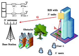
We investigate a multi-user uplink communication system with imperfect hardware, where $K$ single-antenna users transmit signals to a BS equipped with large-scale arrays of $M$ antennas. As shown in Fig. 1, the direct links between the users and the BS are blocked by obstacles such as buildings and trees. Therefore, we employ an RIS with $N$ elements to assist the communications between the users and the BS.

In this section, we investigate the uplink ergodic AR of this multi-user massive MIMO system and the impacts of the system settings, such as the number of the reflecting elements $N$ at the RIS and the number of the antennas $M$ at the BS.

According to (13), the uplink ergodic AR for user $k$ is expressed as (14) at the bottom of this page, where the power of the distortion noise, the AWGN, and the quantization noise are respectively expressed as

Based on (14), we present the following theorem.

It can be readily observed from Theorem 1 that the uplink ergodic AR of user $k$ depends on $M$, $N$, the AoA at the BS, the AoA and AoD at the RIS, the power of users, the large-scale fading coefficients, the Rician factors, the phase shifts and noise at the RIS, the RF impairments, and the quantization bit and accuracy.

In particular, when the Rician factors satisfy $\mu_{k}=0$, $\forall k$ and $\delta=0$, the Rician fading channels expressed in (1) and (2) degenerate to Rayleigh fading channels, where only the nLoS parts of the channels remain. The following remark discusses the uplink ergodic AR with Rayleigh fading channels under the considered system.

Theorem 1 shows that the uplink ergodic AR depends on the phase shift of the RIS. Thus, to enhance the system performance, we can optimize the phase shifts at the RIS for maximizing the sum uplink ergodic AR.

From (18), the sum uplink ergodic AR of the RIS-assisted multi-user uplink massive MIMO system can be expressed as

Since the phase shift at each unit of the RIS lies in the range of $\left[0,2\pi\right)$, the phase shift optimization problem can be expressed as

where $\tilde{R}_{\mathrm{sum}}$ is the sum uplink ergodic AR defined in (32), $\mathbf{\Phi}$ is the phase shift matrix, and $\theta_{n}$ is the phase shift at unit $n$ of the RIS. According to (18) and (32), the expression for the objective function of Problem (IV) is complicated, which makes the problem challenging to be solved. Herein, we apply GA to solve our phase shift optimization problem.

Simulating the evolution of nature population, GA mainly includes five parts: population initialization, fitness evaluation & sort, selection, crossover and mutation. By tailoring it to our phase shift optimization problem, we further discuss the five parts of GA.

1) Population initialization: In the beginning, $N_{\mathrm{tot}}$ individuals are generated in the initial population. For the $N$ phase shifts at the $N$ reflecting elements of the RIS, each individual has one chromosome containing $N$ genes. Furthermore, the value of each gene is initially generated in $\left[0,2\pi\right)$.

2) Fitness evaluation & sort: The fitness value of the individual $i$ is evaluated by the fitness function, which is given by

where $\tilde{R}_{\mathrm{sum},i}$ is the sum uplink ergodic AR corresponding to individual $i$. Since we use the objective function in Problem (IV) as the fitness function, the individual corresponding to a higher sum uplink ergodic AR has a higher fitness value. Then, $N_{\mathrm{tot}}$ individuals are sorted by the fitness values given in (34) as LIST 1.

3) Selection: The selection operation is to choose individuals from the current population as parents. Before the selection operation, we choose the top $N_{\mathrm{e}}$ individuals in LIST 1 as elite individuals, which are directly copied to the next generation. The operation for the elite individuals is to make sure that the optimal individuals in the current population are passed to the next. Then, we scale the fitness values of the individuals in LIST 1 as follows:

where $f_{i}^{\mathrm{list}}$ is the fitness value of the $i$th individual in LIST 1. Based on (35), the selection algorithm is given in Algorithm 1, which is used to select one parent once at a time.

4) Crossover: The crossover operation needs two parents. Simply, we execute the selection operation two times to generate two parents for one crossover operation. The crossover algorithm is given in Algorithm 2, where $p_{\mathrm{c}}$ stands for the crossover probability, and $\mathrm{parent}1$ and $\mathrm{parent}2$ are generated from the selection operation.

5) Mutation: The mutation operation is after the crossover operation. Each gene of the child generated from the crossover operation can mutate under the mutation probability $p_{\mathrm{m}}$. The mutation operation is shown in Algorithm 3. Finally, the child after the mutation operation is added to the next generation.

Based on Algorithms 1-3, we propose a GA for the phase shift optimization problem (IV) to obtain the optimal phase shifts $\left\{\theta_{n}^{\mathrm{opt}}\left|n=1,2,...N\right.\right\}$ along with the maximum sum rate $\tilde{R}_{\mathrm{sum}}^{\max}$. The GA is given in Algorithm 4. Additionally, the complexity of the proposed GA-based algorithm is $N_{\mathrm{tot}}\ast n$, where $N_{\mathrm{tot}}$ is the population size, and $n$ is the number of generations evaluated which is determined by the convergence behavior of the GA [43].

It is noted that the phase shifts vary in a continuous range of $\left[0,2\pi\right)$ in Problem (IV). However, in practical scenarios, the phase shifts are usually discrete values in the range of $\left[0,2\pi\right)$. In that case, the phase shift optimization problem can be formulated as

where the range of the phase shifts is divided into $B$ bits. It is readily to be seen that with a larger $B$, the phase shifts can be adjusted more accurately. When the values of the genes are generated from the discrete range, Algorithm 4 can be applied to solve Problem (IV) with discrete phase shifts as to solve Problem (IV).

In this section, numerical results are provided. Similar to the settings in [44] and [20], we consider a scenario placed in an XYZ Cartesian coordinate system, where the BS is at coordinate $\left(0,0,25\right)$, and the RIS is at $\left(5,100,30\right)$. Users are assumed to be randomly distributed within the circle in Plane $z=1.6$ with the center at $\left(0,0,1.6\right)$. The values for the AoA and AoD of the BS and the RIS are generated from a uniform distribution in $\left(0,2\pi\right)$. Furthermore, we set the spacing distance at the BS and the RIS as $d=\frac{\lambda}{2}$, the number of users as $K=4$, the Rician factors as $\delta=1$ and $\mu_{k}=10$, $\forall k$, the transmit power of users as $p_{k}=30$ dBm, $\forall k$, the parameter of the phase noise as $\upsilon=20$, the amplitude and phase parameters of RF impairments as $\kappa=0.9$ and $\eta=\pi/6$, the noise power as $\sigma^{2}=\sigma_{\mathrm{RF}}^{2}=-104$ dBm, and the ADC quantization bits as $b=2$. The large-scale fading coefficient is modeled as

where $l$ is the distance between the source and the destination. $\alpha_{\mathrm{p}}$ is the path-loss exponent, which is assumed to be $\alpha_{\mathrm{p}}=2.8$ in this section. Additionally, the simulation results in this section are obtained by averaging over 2000 Monte Carlo realizations.

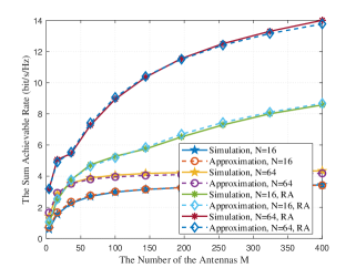
In Fig. 2, we study how the sum rates vary with the number of the antennas $M$ at the BS, setting the number of the reflecting elements $N$ at the RIS as $N=16$ and $N=64$. The curves marked with “Simulation” are obtained based on (14), while the curves marked with “Approximation” are obtained according to (18) in Theorem 1. Two cases are considered: 1) Case 1: the phase shifts at the RIS are fixed, each of which is randomly generated from a uniform distribution in $\left(0,2\pi\right)$; 2) Case 2: the phase shifts at the RIS are obtained by applying the GA in Algorithm 4 to Problem (IV). The parameters of the GA are set as: the population is $N_{\mathrm{tot}}=200$, the number of elites is $N_{\mathrm{e}}=10$, the crossover probability is $p_{\mathrm{c}}=0.4$, the mutation probability is $p_{\mathrm{m}}=0.1$, and the number of the termination iteration times is $t_{T}=2000$. It can be seen that the approximation curves match well with the simulation curves, which supports the results in Theorem 1. Moreover, it is noted that the sum rates with the optimized phase shifts obtained by Algorithm 4 are better than that with the fixed phase shifts. Furthermore, the sum rates increase with $M$ in Case 2 with the optimized phase shifts, while for Case 1 with the fixed phase shifts, the sum rates first increase and then tend to be saturated with $M$. Additionally, the sum rates with $N=64$ are higher than that with $N=16$ in both Case 1 and 2. Therefore, we can improve the performance of the RIS-assisted multi-user massive MIMO system by increasing $M$ and $N$, while using the optimized phase shifts obtained by the proposed GA in Algorithm 4.

In Fig. 3, we investigate the power scaling laws of the users. Two groups of the fixed phase shifts are considered, which are obtained by using the GA in Algorithm 4 with $N=16$ and $N=64$ respectively, when $M=64$. We set the power as $p_{k}=\frac{E_{u}}{M^{\epsilon}}$, $\forall k$, with fixed $E_{u}=10$ dB. The curves marked with “Approximation” in Fig. 3 are obtained according to (26). It can be seen that when the power scaling factor $\epsilon=1.4$, as $M\rightarrow\infty$, the sum rates converge to zero in both cases with $N=16$ and $N=64$. This is because the transmit power is scaled down too fast with $M$. Furthermore, when $\epsilon=1$, as $M\rightarrow\infty$, the sum rates converge to non-zero limits in both cases with $N=16$ and $N=64$. It means the system maintains a required performance when the transmit power is scaled down by the factor $\frac{1}{M}$, which validates our analysis in Section III.

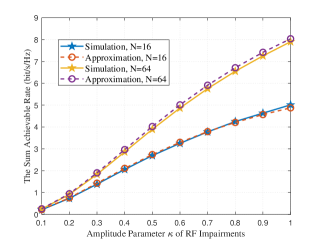
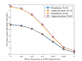
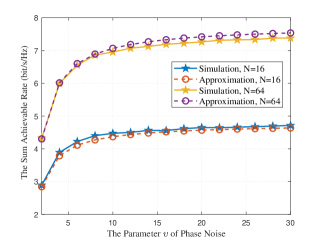
Fig. 4 shows the impacts of the phase noise at the RIS on the sum rates. It can be seen that the sum rates increase as the concentration parameter $\upsilon$ increases. For both $N=16$ and $N=64$ cases, the increase of the sum rates is rapid when $\upsilon$ is small, and then slows down when $\upsilon$ is large. Since the phase noise ${\varepsilon_{n}}$ at the unit $n$ of the RIS follows a Von Mises distribution, a higher concentration parameter $\upsilon$ means the fluctuation for ${\varepsilon_{n}}$ lies in a smaller range. Specifically, when $\upsilon\rightarrow\infty$, we have ${\varepsilon_{n}}\rightarrow 0$, which means there is no phase noise at the RIS. Therefore, the sum rates converge to the case without phase noise as the concentration parameter $\upsilon$ grows to infinity, which is consistent with the results in Fig. 4, where the sum rates first increase and then become saturated as $\upsilon$ increases.

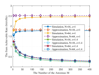
Fig. 5 and 6 focus on the impacts of RF impairments on the sum rates while setting $M=64$. In Fig. 5, we can find that the sun rates increase with the amplitude parameter $\kappa$ in both $N=16$ and $N=64$ cases. It should be mentioned that $\kappa=1$ means RF impairments have no impacts on the amplitude of the receiving signals. Thus, a smaller $\kappa$ stands for severer RF impairments, causing larger reduction of the system performance, as is shown in Fig. 5. In Fig. 6, it is observed that the sun rates decrease with the phase parameter $\eta$ in both $N=16$ and $N=64$ cases. This is because when $\eta$ is large, the phase shifts brought by RF impairments would lie in a large range, which leads to poor system performance.

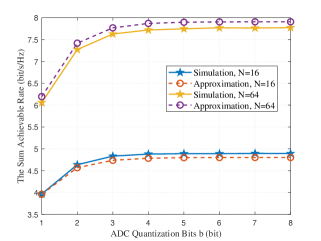
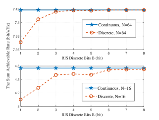
Fig. 7 depicts how the sum rates vary with the ADC quantization bits $b$. It is readily seen that in both $N=16$ and $N=64$ cases, the sum rates first increase fast with $b$, and then become saturated. It is well known that the power consumption and hardware cost of wireless systems increase rapidly as ADC quantization bits $b$ increases.. Thus, Fig. 7 indicates that we can choose $b=3$ for the considered system to obtain a balance between system performance, power consumption and hardware cost.

Finally, we make a comparison between the cases with continuous phase shifts and with discrete phase shifts in Fig. 8. The phase shifts for the curves marked with ”Discrete” is obtained by applying Algorithm 4 to Problem (IV) with discrete phase shifts. The RIS discrete bits $B$ is defined in (IV). In practical scenarios, discrete phase shifts are used, while the continuous phase shifts are considered for ideal scenarios. Therefore, it is essential to study the system performance with discrete phase shifts. From Fig. 8, the sum rates with the optimized discrete phase shifts increase as $B$ increases, and converge to that with the optimized continuous phase shifts. It is noted that $B=6$ and $B=3$ are reasonable choices for the discrete case with $N=16$ and $N=64$, respectively, since they achieve the performance for the corresponding continuous cases, while a higher $B$ leads to more cost.

The paper studied an RIS-assisted multi-user uplink massive MIMO system under Rician fading channels and with imperfect hardware at both the RIS and BS. At the RIS, the paper used Von Mises distribution to model the phase noise, while at the BS, the paper adopted EEVM model for RF impairments and AQNM for low-resolution ADCs. Based on that, asymptotic data rates were obtained with infinite $M$ and $N$, when the RIS was aligned to a specific user and when the RIS was aligned to none of the users. Besides, the paper investigated the power scaling laws of the users, and showed that while guaranteeing a required system performance, the transmit power of the users can be scaled down at most by the factor $\frac{1}{M}$ when $M$ goes infinite, or by the factor $\frac{1}{MN}$ when $M$ and $N$ go infinite. Furthermore, an optimization algorithm was proposed based on GA, which can be applied to solve the continuous and discrete phase shift optimization problems for maximizing the sum rates of the system. Numerical results were provided to support the main results. The numerical results revealed that the sum rate of the considered system can be improved by increasing $M$ and $N$. Moreover, the impacts of the parameters of the imperfect hardware on the system performance were revealed. The numerical results also revealed that when $M=64$, $B=6$ and $B=3$ are reasonable choices for the discrete cases with $N=16$ and $N=64$, respectively.

References

• [1] Y. Zhou, L. Tian, L. Liu, and Y. Qi, “Fog computing enabled future mobile communication networks: A convergence of communication and computing,” IEEE Commun. Mag., vol. 57, no. 5, pp. 20–27, May 2019.
• [2] H. Q. Ngo, H. A. Suraweera, M. Matthaiou, and E. G. Larsson, “Multipair full-duplex relaying with massive arrays and linear processing,” IEEE J. Sel. Areas Commun., vol. 32, no. 9, pp. 1721–1737, Sep. 2014.
• [3] B. Sun, Y. Zhou, J. Yuan, and J. Shi, “Interference cancellation based channel estimation for massive MIMO systems with time shifted pilots,” IEEE Trans. Wireless Commun., vol. 19, no. 10, pp. 6826–6843, Oct. 2020.
• [4] Z. Peng, X. Chen, W. Xu, C. Pan, L.-C. Wang, and L. Hanzo, “Analysis and optimization of massive access to the IoT relying on multi-pair two-way massive MIMO relay systems,” IEEE Trans. Commun., vol. 69, no. 7, pp. 4585–4598, Jul. 2021.
• [5] S. Hu, F. Rusek, and O. Edfors, “Beyond massive MIMO: The potential of data transmission with large intelligent surfaces,” IEEE Trans. Signal Process., vol. 66, no. 10, pp. 2746–2758, May 2018.
• [6] M. Di Renzo, A. Zappone, M. Debbah, M.-S. Alouini, C. Yuen, J. de Rosny, and S. Tretyakov, “Smart radio environments empowered by reconfigurable intelligent surfaces: How it works, state of research, and the road ahead,” IEEE J. Sel. Areas Commun., vol. 38, no. 11, pp. 2450–2525, Nov. 2020.
• [7] z. Özdogan, E. Björnson, and E. G. Larsson, “Intelligent reflecting surfaces: Physics, propagation, and pathloss modeling,” IEEE Wireless Commun. Lett., vol. 9, no. 5, pp. 581–585, May 2020.
• [8] W. Yan, X. Yuan, and X. Kuai, “Passive beamforming and information transfer via large intelligent surface,” IEEE Wireless Commun. Lett., vol. 9, no. 4, pp. 533–537, Apr. 2020.
• [9] C. Pan, H. Ren, K. Wang, J. F. Kolb, M. Elkashlan, M. Chen, M. Di Renzo, Y. Hao, J. Wang, A. L. Swindlehurst, X. You, and L. Hanzo, “Reconfigurable intelligent surfaces for 6G systems: Principles, applications, and research directions,” IEEE Commun. Mag., vol. 59, no. 6, pp. 14–20, Jun. 2021.
• [10] X. Wei, D. Shen, and L. Dai, “Channel estimation for RIS assisted wireless communications—part i: Fundamentals, solutions, and future opportunities,” IEEE Commun. Lett., vol. 25, no. 5, pp. 1398–1402, May 2021.
• [11] Z. Peng, Z. Zhang, C. Pan, L. Li, and A. L. Swindlehurst, “Multiuser full-duplex two-way communications via intelligent reflecting surface,” IEEE Trans. Signal Process., vol. 69, pp. 837–851, Feb. 2021.
• [12] Y. Han, W. Tang, S. Jin, C.-K. Wen, and X. Ma, “Large intelligent surface-assisted wireless communication exploiting statistical CSI,” IEEE Trans. Veh. Technol., vol. 68, no. 8, pp. 8238–8242, Aug. 2019.
• [13] Y. Jia, C. Ye, and Y. Cui, “Analysis and optimization of an intelligent reflecting surface-assisted system with interference,” IEEE Trans. Wireless Commun., vol. 19, no. 12, pp. 8068–8082, Dec. 2020.
• [14] G. Yu, X. Chen, C. Zhong, D. W. Kwan Ng, and Z. Zhang, “Design, analysis, and optimization of a large intelligent reflecting surface-aided b5g cellular internet of things,” IEEE Internet Things J., vol. 7, no. 9, pp. 8902–8916, Sep. 2020.
• [15] X. Hu, C. Zhong, Y. Zhang, X. Chen, and Z. Zhang, “Location information aided multiple intelligent reflecting surface systems,” IEEE Trans. Commun., vol. 68, no. 12, pp. 7948–7962, Dec. 2020.
• [16] Z. Peng, T. Li, C. Pan, H. Ren, W. Xu, and M. D. Renzo, “Analysis and optimization for RIS-aided multi-pair communications relying on statistical CSI,” IEEE Trans. Veh. Technol., vol. 70, no. 4, pp. 3897–3901, Apr. 2021.
• [17] Y. Zhang, J. Zhang, M. D. Renzo, H. Xiao, and B. Ai, “Performance analysis of RIS-aided systems with practical phase shift and amplitude response,” IEEE Trans. Veh. Technol., vol. 70, no. 5, pp. 4501–4511, May 2021.
• [18] J. Zhang, J. Liu, S. Ma, C.-K. Wen, and S. Jin, “Large system achievable rate analysis of ris-assisted MIMO wireless communication with statistical CSIT,” IEEE Trans. Wireless Commun., vol. 20, no. 9, pp. 5572–5585, Sep. 2021.
• [19] K. Xu, J. Zhang, X. Yang, S. Ma, and G. Yang, “On the sum-rate of RIS-assisted MIMO multiple-access channels over spatially correlated rician fading,” IEEE Trans. Commun., vol. 69, no. 12, pp. 8228–8241, Dec. 2021.
• [20] K. Zhi, C. Pan, H. Ren, and K. Wang, “Power scaling law analysis and phase shift optimization of RIS-aided massive MIMO systems with statistical CSI,” IEEE Trans. Commun., vol. 70, no. 5, pp. 3558–3574, May 2022.
• [21] X. Zhang, M. Matthaiou, M. Coldrey, and E. Björnson, “Impact of residual transmit RF impairments on training-based MIMO systems,” IEEE Trans. Commun., vol. 63, no. 8, pp. 2899–2911, Aug. 2015.
• [22] X. Xia, D. Zhang, K. Xu, W. Ma, and Y. Xu, “Hardware impairments aware transceiver for full-duplex massive MIMO relaying,” IEEE Trans. Signal Process., vol. 63, no. 24, pp. 6565–6580, Dec. 2015.
• [23] T. Schenk, RF imperfections in high-rate wireless systems : impact and digital compensation.   Germany: Springer, 2008.
• [24] C. Studer, M. Wenk, and A. Burg, “MIMO transmission with residual transmit-RF impairments,” in Proc. Int. ITG Workshop Smart Antennas, Feb. 2010, pp. 189–196.
• [25] E. Björnson, M. Matthaiou, and M. Debbah, “Massive MIMO with non-ideal arbitrary arrays: Hardware scaling laws and circuit-aware design,” IEEE Trans. Wireless Commun., vol. 14, no. 8, pp. 4353–4368, Aug. 2015.
• [26] H. Shen, W. Xu, S. Gong, C. Zhao, and D. W. K. Ng, “Beamforming optimization for IRS-aided communications with transceiver hardware impairments,” IEEE Trans. Commun., vol. 69, no. 2, pp. 1214–1227, Feb. 2021.
• [27] G. Zhou, C. Pan, H. Ren, K. Wang, and Z. Peng, “Secure wireless communication in RIS-aided MISO system with hardware impairments,” IEEE Wireless Commun. Lett., vol. 10, no. 6, pp. 1309–1313, Jun. 2021.
• [28] M. A. Saeidi, M. J. Emadi, H. Masoumi, M. R. Mili, D. W. K. Ng, and I. Krikidis, “Weighted sum-rate maximization for multi-IRS-assisted full-duplex systems with hardware impairments,” IEEE Trans. Cogn. Commun. Netw., vol. 7, no. 2, pp. 466–481, Jun. 2021.
• [29] P. Dong, H. Zhang, W. Xu, and X. You, “Efficient low-resolution ADC relaying for multiuser massive MIMO system,” IEEE Trans. Veh. Technol., vol. 66, no. 12, pp. 11 039–11 056, Dec. 2017.
• [30] P. Dong, H. Zhang, Q. Wu, and G. Y. Li, “Spatially correlated massive MIMO relay systems with low-resolution ADCs,” IEEE Trans. Veh. Technol., vol. 69, no. 6, pp. 6541–6553, Jun. 2020.
• [31] L. Xu, X. Lu, S. Jin, F. Gao, and Y. Zhu, “On the uplink achievable rate of massive MIMO system with low-resolution ADC and RF impairments,” IEEE Commun. Lett., vol. 23, no. 3, pp. 502–505, Mar. 2019.
• [32] K. Zhi, C. Pan, H. Ren, and K. Wang, “Uplink achievable rate of intelligent reflecting surface-aided millimeter-wave communications with low-resolution ADC and phase noise,” IEEE Wireless Commun. Lett., vol. 10, no. 3, pp. 654–658, Mar. 2021.
• [33] J. Dai, Y. Wang, C. Pan, K. Zhi, H. Ren, and K. Wang, “Reconfigurable intelligent surface aided massive MIMO systems with low-resolution DACs,” IEEE Commun. Lett., vol. 25, no. 9, pp. 3124–3128, Sep. 2021.
• [34] M.-A. Badiu and J. P. Coon, “Communication through a large reflecting surface with phase errors,” IEEE Wireless Commun. Lett., vol. 9, no. 2, pp. 184–188, Feb. 2020.
• [35] J. D. Vega Sánchez, P. Ramírez-Espinosa, and F. J. López-Martínez, “Physical layer security of large reflecting surface aided communications with phase errors,” IEEE Wireless Commun. Lett., vol. 10, no. 2, pp. 325–329, Feb. 2021.
• [36] Y. Liu, E. Liu, and R. Wang, “Energy efficiency analysis of intelligent reflecting surface system with hardware impairments,” in Proc. IEEE GLOBECOM, Dec. 2020, pp. 1–6.
• [37] Y. Liu, E. Liu, R. Wang, and Y. Geng, “Channel estimation and power scaling of reconfigurable intelligent surface with non-ideal hardware,” in Proc. IEEE WCNC, Mar. 2021, pp. 1–6.
• [38] S. Zhou, W. Xu, K. Wang, M. Di Renzo, and M.-S. Alouini, “Spectral and energy efficiency of IRS-assisted MISO communication with hardware impairments,” IEEE Wireless Commun. Lett., vol. 9, no. 9, pp. 1366–1369, Sep. 2020.
• [39] Z. Xing, R. Wang, J. Wu, and E. Liu, “Achievable rate analysis and phase shift optimization on intelligent reflecting surface with hardware impairments,” IEEE Trans. Wireless Commun., vol. 20, no. 9, pp. 5514–5530, Sep. 2021.
• [40] A. Papazafeiropoulos, C. Pan, A. Elbir, V. Nguyen, P. Kourtessis, and S. Chatzinotas, “Asymptotic analysis of max-min weighted SINR for IRS-assisted MISO systems with hardware impairments,” IEEE Wireless Commun. Lett., 2021, to be published, doi: 10.1109/LWC.2021.3095678.
• [41] A. Papazafeiropoulos, C. Pan, P. Kourtessis, S. Chatzinotas, and J. M. Senior, “Intelligent reflecting surface-assisted MU-MISO systems with imperfect hardware: Channel estimation and beamforming design,” IEEE Trans. Wireless Commun., vol. 21, no. 3, pp. 2077–2092, Mar. 2022.
• [42] T. C. W. Schenk and E. R. Fledderus, “RF impairments in high-rate wireless systems - understanding the impact of TX/RX-asymmetry,” in Proc. 3rd Int. Symp. ISCCSP, Mar. 2008, pp. 117–122.
• [43] Z. Ye, C. Pan, H. Zhu, and J. Wang, “Tradeoff caching strategy of the outage probability and fronthaul usage in a cloud-RAN,” IEEE Trans. Veh. Technol., vol. 67, no. 7, pp. 6383–6397, Jul. 2018.
• [44] C. Pan, H. Ren, K. Wang, W. Xu, M. Elkashlan, A. Nallanathan, and L. Hanzo, “Multicell MIMO communications relying on intelligent reflecting surfaces,” IEEE Trans. Wireless Commun., vol. 19, no. 8, pp. 5218–5233, May 2020.
• [45] Q. Zhang, S. Jin, K. Wong, H. Zhu, and M. Matthaiou, “Power scaling of uplink massive MIMO systems with arbitrary-rank channel means,” IEEE J. Sel. Top. Sign. Proces., vol. 8, no. 5, pp. 966–981, Oct. 2014.
[Uncaptioned image] Zhangjie Peng received the B.S. degree from Southwest Jiaotong University, Chengdu, China, in 2004, and the M.S. and Ph.D. degrees from Southeast University, Southeast University, Nanjing, China, in 2007, and 2016, respectively, all in Communication and Information Engineering. He is currently an Associate Professor at the College of Information, Mechanical and Electrical Engineering, Shanghai Normal University, Shanghai 200234, China. His research interests include reconfigurable intelligent surface (RIS), cooperative communications, information theory, physical layer security, and machine learning for wireless communications.
[Uncaptioned image] Xianzhe Chen received the B.E. degree in information engineering from Zhejiang University, Zhejiang, China, in 2019, and the M.E. degree in information and communication engineering from Shanghai Normal University, Shanghai, China, in 2022. He is currently pursuing the Ph.D. degree with the Department of Electrical and Computer Engineering, The University of British Columbia, Vancouver, Canada. His major research interests include reconfigurable intelligent surfaces, massive multiple-input multiple-output systems and relaying communications.
[Uncaptioned image] Cunhua Pan received the B.S. and Ph.D. degrees from the School of Information Science and Engineering, Southeast University, Nanjing, China, in 2010 and 2015, respectively. From 2015 to 2016, he was a Research Associate at the University of Kent, U.K. He held a post-doctoral position at Queen Mary University of London, U.K., from 2016 and 2019.From 2019 to 2021, he was a Lecturer in the same university. From 2021, he is a full professor in Southeast University. His research interests mainly include reconfigurable intelligent surfaces (RIS), intelligent reflection surface (IRS), ultra-reliable low latency communication (URLLC) , machine learning, UAV, Internet of Things, and mobile edge computing. He has published over 120 IEEE journal papers. He is currently an Editor of IEEE Wireless Communication Letters, IEEE Communications Letters and IEEE ACCESS. He serves as the guest editor for IEEE Journal on Selected Areas in Communications on the special issue on xURLLC in 6G: Next Generation Ultra-Reliable and Low-Latency Communications. He also serves as a leading guest editor of IEEE Journal of Selected Topics in Signal Processing (JSTSP) Special Issue on Advanced Signal Processing for Reconfigurable Intelligent Surface-aided 6G Networks, leading guest editor of IEEE Vehicular Technology Magazine on the special issue on Backscatter and Reconfigurable Intelligent Surface Empowered Wireless Communications in 6G, leading guest editor of IEEE Open Journal of Vehicular Technology on the special issue of Reconfigurable Intelligent Surface Empowered Wireless Communications in 6G and Beyond, and leading guest editor of IEEE ACCESS Special Issue on Reconfigurable Intelligent Surface Aided Communications for 6G and Beyond. He is Workshop organizer in IEEE ICCC 2021 on the topic of Reconfigurable Intelligent Surfaces for Next Generation Wireless Communications (RIS for 6G Networks), and workshop organizer in IEEE Globecom 2021 on the topic of Reconfigurable Intelligent Surfaces for future wireless communications. He is currently the Workshops and Symposia officer for Reconfigurable Intelligent Surfaces Emerging Technology Initiative. He is workshop chair for IEEE WCNC 2024, and TPC co-chair for IEEE ICCT 2022. He serves as a TPC member for numerous conferences, such as ICC and GLOBECOM, and the Student Travel Grant Chair for ICC 2019. He received the IEEE ComSoc Leonard G. Abraham Prize in 2022.
[Uncaptioned image] Maged Elkashlan received the PhD degree in Electrical Engineering from the University of British Columbia in 2006. From 2007 to 2011, he was with the Commonwealth Scientific and Industrial Research Organization (CSIRO) Australia. During this time, he held visiting faculty appointments at University of New South Wales, University of Sydney, and University of Technology Sydney. In 2011, he joined the School of Electronic Engineering and Computer Science at Queen Mary University of London. He also holds a visiting faculty appointment at Beijing University of Posts and Telecommunications. His research interests fall into the broad areas of communication theory and signal processing. Dr. Elkashlan is an Editor of the IEEE TRANSACTIONS ON VEHICULAR TECHNOLOGY and the IEEE TRANSACTIONS ON MOLECULAR, BIOLOGICAL AND MULTI-SCALE COMMUNICATIONS. He was an Editor of the IEEE TRANSACTIONS ON WIRELESS COMMUNICATIONS from 2013 to 2018 and the IEEE COMMUNICATIONS LETTERS from 2012 to 2016. He received numerous awards, including the 2022 IEEE Communications Society Leonard G. Abraham Prize, and best paper awards at the 2014 and 2016 IEEE ICC, 2014 CHINACOM, and 2013 IEEE VTC-Spring.
[Uncaptioned image] Jiangzhou Wang (Fellow, IEEE) is a Professor at the University of Kent, U.K. His research interest is in mobile communications. He has published over 400 papers and 4 books. He was a recipient of the 2022 IEEE Communications Society Leonard G. Abraham Prize and the 2012 IEEE Globecom Best Paper Award. Professor Wang is a Fellow of the Royal Academy of Engineering, U.K., Fellow of the IEEE, and Fellow of the IET. He was the Technical Program Chair of the 2019 IEEE International Conference on Communications (ICC2019), Shanghai, the Executive Chair of the IEEE ICC2015, London, and the Technical Program Chair of the IEEE WCNC2013. He was an IEEE Distinguished Lecturer from 2013 to 2014. He has served as an Editor for a number of international journals, including IEEE Transactions on Communications from 1998 to 2013.