PCRDiffusion: Diffusion Probabilistic Models for Point Cloud Registration
Abstract
We propose a new framework that formulates point cloud registration as a denoising diffusion process from noisy transformation to object transformation. During training stage, object transformation diffuses from ground-truth transformation to random distribution, and the model learns to reverse this noising process. In sampling stage, the model refines randomly generated transformation to the output result in a progressive way. We derive the variational bound in closed form for training and provide implementations of the model. Our work provides the following crucial findings: (i) In contrast to most existing methods, our framework, Diffusion Probabilistic Models for Point Cloud Registration (PCRDiffusion) does not require repeatedly update source point cloud to refine the predicted transformation. (ii) Point cloud registration, one of the representative discriminative tasks, can be solved by a generative way and the unified probabilistic formulation. Finally, we discuss and provide an outlook on the application of diffusion model in different scenarios for point cloud registration. Experimental results demonstrate that our model achieves competitive performance in point cloud registration. In correspondence-free and correspondence-based scenarios, PCRDifussion can both achieve exceeding 50% performance improvements.
Index Terms:
Point cloud registration, diffusion probabilistic models, discriminative tasks.1 Introduction
With the rapid development of 3D data acquisition technology [1, 2], point cloud registration, as a fundamental visual recognition task plays an essential role in the 3D vision field, and has been widely applied in various vision tasks, such as 3D scene reconstruction [3, 4], object pose estimation [5, 6], and simultaneous localization and mapping (SLAM) [7, 8]. Given two 3D point clouds, the goal is to find a rigid transformation to align one point cloud to another. The problem has gained renewed interest recently thanks to the fast growing of 3D point representation learning and differentiable optimization.
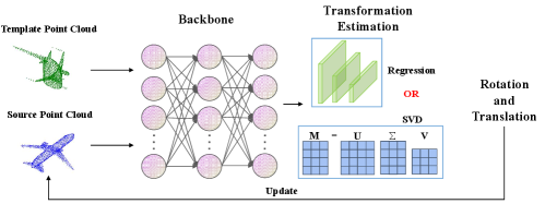
Rigid point cloud registration methods have been evolving in response to the growing complexity of components and usage scenarios. They have advanced from the most basic technique of utilizing regression to predict transformation parameters in the correspondence-free methods [9, 10, 11, 12, 13], employing correspondence-based methods [14, 15, 16, 17] and leveraging SVD decomposition to obtain rigid transformations in partially overlapping scenes. Specifically, in the correspondence-free methods, they are often necessary to seek differences between global features and require them to be sensitive to posture. On the basis of the correspondence-based methods, it is necessary to find the overlapping parts of the point cloud through precise matching and inlier estimation. However, point cloud registration methods typically rely on updating source point cloud to further refine the predicted transformation parameters. A natural question is: is there a simpler approach that does not even update source point cloud?
We answer these questions by designing a novel point cloud registration framework that directly predict object transformation from a random transformation. Starting from purely random transformation, which do not contain learnable parameters that need to be optimized in training, we expect to gradually refine the predicted transformation until they perfectly align two point clouds. This strategy does not require to update source point cloud and heuristic object priors, and it has also promoted the development of the point cloud registration pipeline.
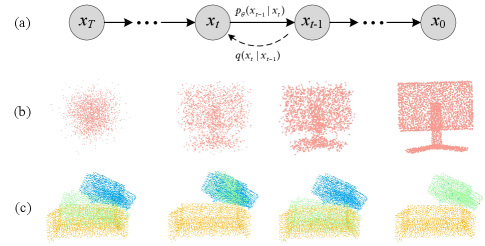
Motivated by the discussion above, we propose a new framework that formulates point cloud registration as a denoising diffusion process from noisy transfromation to object transfromation. As shown in Figure 1, we argue that the process of transforming noise to the object transformation in point cloud registration is analogous to the process of transforming noise to point clouds in denoising diffusion models. These likelihood-based models gradually remove noise from point clouds to generate point clouds with different shapes. Diffusion models have achieved significant success in various generative tasks [18, 19, 20, 21, 22] and have recently started to be explored in some discriminative tasks [23, 24, 25, 26, 27, 28, 29]. However, to the best of our knowledge, there is not existing technique has successfully applied them to point cloud registration.
In this paper, we propose PCRDiffusion to handle the point cloud registration task with a diffusion model by treating the prediction of transformation parameters as a generation task. During the training stage, we employ a variance schedule [18, 30] to control the addition of Gaussian noise to the ground truth transformation, resulting in a noisy transformation. This noisy transformation is then encoded and utilized to guide the generation of transformations from the output feature of the backbone encoder, such as PointNet [31], DGCNN [32] and PointNet++ [33]. Finally, these features are fed into the decoder, which is trained to predict the ground truth transformation without noise. Note that the decoder can be designed based on either correspondence-free methods or correspondence-based methods, depending on the specific context. With this training objective, PCRDiffusion can predict the ground truth transformation from random transformation. During sampling stage, PCRDiffusion generates transformation by reversing the learned diffusion process, which adjusts a noisy prior distribution to the learned distribution over transformation. The “noise-to-ground truth transformation” pipeline of PCRDiffusion has the appealing advantage of Once-for-All: (i) We train the network only once, and no iteration strategy is required to update source point cloud during training and inference. (ii) We can adjust the number of denoising sampling steps to improve the registration accuracy or accelerate the inference speed.
To validate the comprehensiveness of the proposed framework, we conduct experiments on both correspondence-based and correspondence-free methods. Specifically, for the correspondence-free method, we employ a fully overlapping experimental setup on the synthetic dataset ModelNet40 [34]. For the correspondence-based method, we utilize a partially overlapping experimental setup on real-world dataset 3DMatch [35] and KITTI [36]. Experimental results illustrate that our framework achieves competitive performance and effectively improves inference speed. To summarize, our contributions are as follows:
-
•
We formulate point cloud registration as a generative denoising process, which is the first study to apply the diffusion model to point cloud registration to the best of our knowledge.
-
•
The ”noise-to-ground truth transformation” paradigm has several appealing advantage, such as no iteration strategy is required to update source point cloud and adjust the number of denoising sampling steps to improve the registration accuracy or accelerate the inference speed flexibly.
-
•
We conduct experiments on both correspondence-based and correspondence-free methods. Experimental results illustrate that PCRDiffusion achieves competitive performance.
The rest of this paper is organized as follows. In Section 2, we make a review of the related works of point cloud registration and diffusion models. Section 3 gives the formulation of the diffusion probabilistic models for point cloud registration, and then introduces PCRDiffsion framework. Section 4 evaluates the proposed architecture with extensive experiments. Finally, Section 5 concludes this paper and discusses future work.
2 Related Works
2.1 Point Cloud Registration
Most traditional methods need a good initial transformation and converge to the local minima near the initialization point. One of the most profound methods is the Iterative Closest Point (ICP) algorithm [37], which begins with an initial transformation and iteratively alternates between solving two trivial subproblems: finding the closest points as correspondence under current transformation, and computing optimal transformation by SVD [38] based on identified correspondences. Though ICP can complete a high-precision registration, it is susceptible to the initial perturbation and easily prone to local optima. Thus, variants of ICP have been proposed [39, 40, 41, 42, 43], and they can improve the defects of ICP and enhance the registration performance [44]. Generalized-ICP [39] integrates a probabilistic module into an ICP-style framework to enhance the algorithm’s robustness. Go-ICP [40] combines the ICP that integrated the maximum correntropy criterion [45] with the Branch-and-Bound scheme and searches for an optimal solution in the 3D motion space. Besides, Trimmed ICP [46] introduces the least trimmed squares into each part of the ICP pipeline to tackle the partial overlap problem. However, all these methods retain a few essential drawbacks. Firstly, they depend strongly on the initialization. Secondly, it is difficult to integrate them into the deep learning pipeline as they lack differentiability. Thirdly, explicit estimation of corresponding points leads to quadratic complexity scaling with the number of points [47], which can introduce significant computational challenges.
In order to address the aforementioned problems, learning-based methods have made significant advancements in recent years, which are usually divided into correspondence-based methods [14, 15, 16, 17] and correspondence-free methods [9, 10, 11, 12, 13]. Specifically, in the correspondence-free methods, they are often necessary to seek differences between global features and require them to be sensitive to posture. PointNetLK [9] incorporates the Lucas & Kanade (LK) algorithm the PointNet [31] to iteratively align the input point clouds. In PCRNet [48], the LK algorithm is substituted with a fully-connected network and the model improves robustness by regressing. Correspondence-based methods need to find the correspondences between point clouds through precise matching and inlier estimation. IDAM [49] introduces a dual stage point elimination method to facilitate the generation of partial correspondences. However, the efficacy of IDAM remains limited under conditions of low overlapping. EGST [50] construct reliable geometric structure descriptors to extract correspondences and is less sensitive to outliers. OPRNet [51] resorts to the Sinkhorn algorithm [52] tailored to partial-to-partial registration. RPMNet [53] utilizes 3D local patch descriptor [54] to find correspondences in unorganized point clouds. However, all methods rely on updating source point cloud to further refine the predicted transformation parameters, as shown in Figure 2. In this paper, we aim to push forward the development of the point cloud registration pipeline further with diffusion probabilistic models and no iteration strategy is required to update source point cloud during training and inference.
2.2 Diffusion Models
Diffusion models [18, 30, 55, 56] have emerged as the cutting-edge family of deep generative models, representing a class of highly advanced deep generative models. They have broken the long-time dominance of generative adversarial networks (GANs) [57] in the challenging task of image synthesis [58, 55, 56] and have also shown potential in computer vision [23, 24, 59]. Specifically, in 3D computer vision, there has been a recent surge of research using generative models for point cloud generation or completion [60, 21]. These models are employed to infer missing parts and reconstruct complete shapes and hold significant implications for various downstream tasks, such as 3D reconstruction, augmented reality, and scene understanding [61, 22, 62]. [60] involves conceptualizing point clouds as particles within a thermodynamic system, utilizing a heat bath to facilitate diffusion from the original distribution to a noise distribution. The point diffusion-refinement model [22] is introduced by conditional denoising diffusion probabilistic models to generate a coarse completion from partial observations. Furthermore, this model establishes a point-wise mapping between the generated point cloud and the ground truth. While diffusion models have achieved great success in generation tasks, their potential for discriminative tasks has yet to be fully explored. Currently, there are some pioneering works that apply diffusion models to image segmentation [29] and object detection [63]. However, despite the considerable interest in this idea, there hasn’t been a successful application of diffusion models to point cloud registration solutions before, and its progress lags significantly behind image processing. To the best of our knowledge, this is the first work that adopts a diffusion model for point cloud registration.
3 Diffusion Probabilistic Models for Point Cloud Registration
In this section, we begin by introducing the definition of point cloud registration and its mathematical formulations under various modes (Section 3.1). Subsequently, within the context of point cloud registration, we reformulate the diffusion model and establish the training objectives (Section 3.2 and Section 3.3). We then provide a detailed exposition of our proposed framework (Section 3.4-Section 3.6). Finally, we provide the specific details of all experiments (Section 3.7).
3.1 Preliminaries for Point Cloud Registration
We first introduce notations utilized throughout this paper. Given two point clouds: source point cloud and template point cloud , where each point is represented as a vector of coordinates. Point cloud registration task aims to estimate a rigid transformation which accurately aligns and , with a 3D rotation and a 3D translation . The transformation can be solved by:
| (1) |
where is the set of ground-truth correspondences between and . In this paper, for the convenience of formalization, we merge rotation and translation into a single transformation denoted as G. Note that the meaning of G varies depending on the specific context. In the correspondence-free methods, G represents a 7-dimensional vector composed of a rotation quaternion and a translation. In the correspondence-based methods, G represents a transformation matrix as follow:
| (2) |
As a result, our objective becomes: finding the rigid-body transformation which best aligns and such that:
| (3) |
where we use shorthand to denote transformation of by rigid transform G.
3.2 Formulate Point Cloud Registration as Denoising Diffusion Process
The denoising diffusion probabilistic model is a generative model where generation is modeled as a denoising process, in a specific form for point cloud registration:
| (4) |
The denoising process begins with standard Gaussian noise and continues until an optimal transformation is achieved. Specifically, a sequence of transformation variables denoted as , , , is generated through the denoising process, where each variable exhibits a progressively reduced level of noise, where is sampled from a standard Gaussian prior, and represents the final transformation.
We provide a detailed review of the formulation of diffusion models. Starting from a data distribution , we define forward process which produces data samples by gradually adding Gaussian noise at each timestep . In particular, the added noise is scheduled according to a variance schedule :
| (5) | ||||
A notable property of the forward process is that it admits sampling at an arbitrary timestep knowing in convenient closed-form evaluation: using the notation and , we have
| (6) | ||||
The forward process variances can be learned by reparameterization [64], or held constant as hyperparameters, and expressiveness of the reverse process is ensured in part by the choice of Gaussian conditionals in , because both processes have the same functional form when are small [30]. In this work, we fix the forward process variances to constants.
Furthermore, we define reverse process as a Markov chain with learned Gaussian transitions starting at a standard Gaussian prior :
| (7) | ||||
which aims to invert the noise corruption process. Since calculating (ground truth reverse process) exactly should depend on the entire data distribution, we can approximate using a neural network with parameter , which is optimized to predict a mean and a diagonal covariance matrix . Intuitively, the forward process can be seen as gradually injecting more random noise to the data, with the reverse process learning to progressively remove noise to obtain realistic samples by mimicking the ground truth reverse process .
3.3 Reverse Process
The goal of training the reverse diffusion process is to maximize the log-likelihood of the transformation: . However, since directly optimizing the exact log-likelihood is intractable, we instead maximize its variational lower bound:
| (8) | ||||
where the inequality is by Jensen’s inequality and the above derivation after the fifth row is based on the Bayes’ rule [30].
In the final objective of Equation 8, as the forward process is fixed and is defined as a Gaussian prior, does not affect the learning of . can be regarded as the reconstruction of the original data, which can be computed by estimating and constructing a discrete decoder. Therefore, the ultimate optimization objective is . Based on Bayes’ theorem, it is found that the posterior is a Gaussian distribution as well:
| (9) |
where
| (10) | ||||
The final training objective can be reduced to maximum likelihood given the complete data likelihood with joint posterior :
| (11) |
How to choice is a crucial question. In this paper, we set , where . To represent , must be predicted given . Since is available as input to the model , we may choose the parameterization:
| (12) | |||
where is the output of . Finally, the training objective is parameterized:
| (13) |
Based on the aforementioned process, the sampling procedure can be expressed as follows:
| (14) |
Note that since point cloud registration is not a purely generative task, we make further adjustments during the implementation process based on the aforementioned theory, such as the training objective.
3.4 PCRDiffusion Architecture
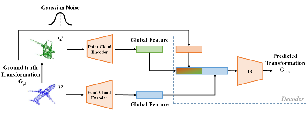
To demonstrate the generalization of our proposed framework, we conduct separate investigations on both correspondences-based and correspondences-free methods. While the overall algorithmic flow can be shared between the two methods, there are distinct differences in the implementation details of each component. We propose to separate the whole framework into two parts, point cloud encoder and transformation estiamtion decoder, where the former runs only once to extract a global representation or point-wise representation from the raw input point cloud and , and encodes the noisy transformation calculated by in Equation 6. The latter takes these representations as condition to predict object transformation. Notably, for correspondence-free method, the number of input points is equal to , whereas for correspondence-based method, is not necessarily equal to .
Point Cloud Encoder. Point cloud encoder takes as input the raw point cloud and extracts its global/point-wise features for the following pipeline. We implement PCRDiffusion for correspondences-free methods with five shared Multi-Layered Perceptrons (MLPs) similar to the PointNet [31] architecture having size 64, 64, 64, 128, 1024. Moreover, PCRDiffusion for correspondences-based methods is implemented by Dynamic Graph CNN [32].
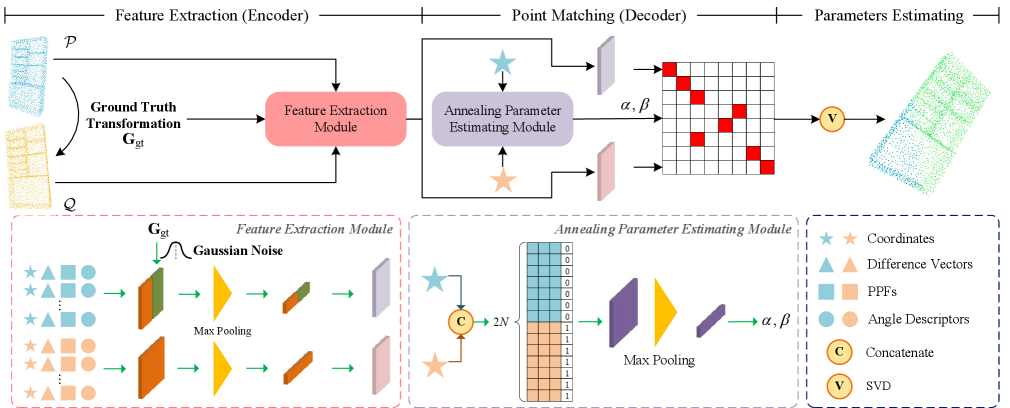
Transformation Estiamtion Decoder. The decoding method varies depending on whether the search for correspondences is required. As shown in Figure 3, for correspondences-free method, it searches the difference between the global features of source point cloud and template point cloud, and estimate the rigid transformation by difference regression with Multi-Layer Perceptrons (MLPs). As shown in Figure 4, for correspondences-based method, we explicitly construct three geometric descriptors utilizing different methods, and combine them into transformation-invariant structured feature. A feature extraction module is utilized to encode the structured feature and simultaneously model the structure consistency across the two point clouds. Based on previous pipeline, we use RPM which has learnable parameters to extract correspondences. Finally, we recover the alignment transformation from the point matching computed in prior component. We opt EGST [50] to establish our decoder network, which produces meaningful results in real-world challenges.
3.5 Training
During training, we first construct the diffusion process from ground-truth transformation to noisy transformation and then train the model to reverse this process. Algorithm 1 provides the pseudo code of PCRDiffsuion training procedure.
Ground Truth Transformation Corruption. We add Gaussian noises to the ground truth transformation by . The noise scale is controlled by , which adopts the monotonically decreasing cosine schedule for in different time step , as proposed in [65]. A crucial point to note is that we uniformly transform the initial input ground truth transformation matrix into 7-dimensional vectors (composed of a rotation quaternion and a translation) before encoding, instead of directly utilizing the transformation matrix. This strategy offers several advantages. Firstly, it ensures linearity in the spread of objects while maintaining same significance. Secondly, it reduces the complexity required for the design of the transformation encoder network.
Training Loss. We employ a supervised training approach in various modes and have tailored different loss functions for each mode. During training, a neural network is trained to predict from by minimizing the training objective with loss :
| (15) |
Note that since point cloud registration is not a purely generative task, we make further adjustments during the implementation process based on the aforementioned theory in Equation 8. For correspondence-free methods, we optimize PCRDiffusion unioning the following two loss functions:
| (16) |
| (17) |
For correspondence-based methods, the loss function for joint optimization is identical to that of EGST [50]. It is noteworthy that during the training process, PCRDiffsuion requires only a single pass through the network. Iterative updates by applying the predicted transformation to the source point cloud are unnecessary.
3.6 Sampling
The inference procedure of PCRDiffusion is a denoising sampling process from noise to object transformation . Starting from transformation sampled in Gaussian distribution, the model progressively refines its predictions, as shown in Algorithm 2.
Sampling Step. At sampling stage, data sample is reconstructed from noise with the model and an updating rule [35, 76] in an iterative way, i.e., . In each sampling step, the random transformation or the estimated transformation from the last sampling step are sent into the transformation estimation decoder. After obtaining the transformation of the current step, DDPM is adopted to estimate the transformation for the next step.
Once-for-All. Thanks to the random transformation design, we can evaluate PCRDiffusion with an arbitrary number of random transformation and the number of sampling steps, which do not need to be equal to the training stage. As a comparison, previous point cloud registration methods typically rely on iterative strategy to further refine the predicted transformation parameters. We train the network only once, and no iteration strategy is required to update source point cloud during training and inference.
3.7 Implementation Details
In our framework, the learnable parameters are adjusted by the back propagation algorithm [66]. We implement and evaluate our model with PyTorch on an NVIDIA RTX 3090 GPU. The network is trained with Adam optimizer [67] for 100 epochs on ModelNet40, 50 epochs on 3DMatch and KITTI. The learning rate starts from 0.0001 and decays when loss has stopped improving. The adjustment of the batch size depends on the specific methods used. For correspondence-free method, the batch size is set to 32, while for correspondence-based method, it is set to 8.
4 Experiments
In this section, we first introduce the experimental settings and the datasets for point cloud registration. After that, we compare PCRDiffusion to other diffusion-free methods on the ModelNet40 dataset. Then, we conduct ablation study to evaluate the effectiveness of the modules in PCRDiffusion. Lastly, we compare PCRDiffusion to other methods on the real-world dataset 3DMatch.
4.1 Setup
We evaluate the proposed method on synthetic datasets ModelNet40 [34], and real-world dataset 3DMatch [35]. ModelNet40 contains 12,308 CAD models of 40 different object categories. Each point cloud contains 2,048 points that randomly sampled from the mesh faces and normalized into a unit sphere. 3DMatch dataset contains 62 indoor subscenes. Some subscenes represent the same scenario with different overlap rates, we ignore this characteristic and treat all subscenes as different scenes. We randomly generate three Euler angle rotations within and translations within on each axis as the rigid transformation during training.
We compare our method to traditional methods: ICP[37] and FGR[68], and recent learning-based methods: PointNetLK [9], PCRNet [48], DeepGMR [69], DCP [70], FMR [10] and RPMNet [53]. We utilize the implementations of ICP and FGR in Intel Open3D [71]. For other baseline, we follow the pipeline provided by original paper. For consistency with previous work, we measure Mean Isotropic Error (MIE) and Mean Absolute Error (MAE). MIE(R) is the geodesic distance in degrees between estimated and ground-truth rotation matrices. It measures the differences between the predicted and the ground-truth rotation matrices. MIE(t) is the Euclidean distance between estimated and ground-truth translation vectors. It measures the differences between the predicted and the ground-truth translation vectors. Here, we give the specific calculation formula of MIE(R) and MIE(t):
| MIE | (18) | |||
Angular measurements are in units of degrees. All metrics should be zero if reference point cloud align to source point cloud perfectly.
| Method | RMSE(R) | RMSE(t) | MAE(R) | MAE(t) | ERROR(R) | ERROR(t) | # Update |
| (a) Unseen Objects | |||||||
| ICP [37] () | 21.2084 | 0.2874 | 11.7468 | 0.1686 | 23.1548 | 0.3497 | 10 |
| PointNetLK [9] () | 7.4796 | 0.5820 | 1.7362 | 0.4907 | 4.0421 | 0.9741 | 5 |
| PCRNet [48]() | 19.8457 | 0.2288 | 10.2498 | 0.1168 | 19.0487 | 0.2442 | 8 |
| DeepGMR [69]() | 34.1993 | 0.4495 | 23.5162 | 0.3291 | 45.7786 | 0.6758 | 0 |
| FGR [68]() | 9.5964 | 0.1186 | 1.9971 | 0.0268 | 4.3337 | 0.0582 | 10 |
| DCP [70]() | 15.7183 | 0.2002 | 10.7846 | 0.1340 | 20.8744 | 0.2740 | 0 |
| FMR [10]() | 6.8525 | 0.5851 | 1.5962 | 0.4886 | 3.8090 | 0.9751 | 5 |
| RPMNet [53]() | 8.0357 | 0.0841 | 1.4399 | 0.0170 | 2.9619 | 0.0357 | 3 |
| PCRDiffusion Correspondence-Free () | 3.3737 | 0.0460 | 1.6861 | 0.0216 | 3.2786 | 0.0448 | 0 |
| PCRDiffusion Correspondence-Based () | 1.0986 | 0.0218 | 0.7244 | 0.0153 | 1.2732 | 0.0318 | 0 |
| (b) Unseen Categories | |||||||
| ICP [37] () | 21.8745 | 0.2707 | 11.0308 | 0.1588 | 21.9911 | 0.3307 | 10 |
| PointNetLK [9] () | 8.7766 | 0.5702 | 2.3269 | 0.4768 | 5.5023 | 0.9555 | 5 |
| PCRNet [48] () | 22.0931 | 0.2943 | 15.4301 | 0.1946 | 29.3938 | 0.3978 | 8 |
| DeepGMR [69] () | 35.2986 | 0.4520 | 22.6519 | 0.3314 | 43.7901 | 0.6816 | 0 |
| FGR [68] () | 10.6061 | 0.1214 | 2.3841 | 0.0312 | 5.2151 | 0.0672 | 10 |
| DCP [70] () | 21.4669 | 0.3194 | 15.2743 | 0.2357 | 29.3084 | 0.4834 | 0 |
| FMR [10] () | 7.5793 | 0.5667 | 1.8031 | 0.4750 | 4.4476 | 0.9434 | 5 |
| RPMNet [53] () | 5.3739 | 0.0736 | 1.1452 | 0.0144 | 2.5072 | 0.0316 | 3 |
| PCRDiffusion Correspondence-Free () | 3.1880 | 0.0447 | 1.6887 | 0.0216 | 3.1686 | 0.0446 | 0 |
| PCRDiffusion Correspondence-Based () | 0.2848 | 0.0045 | 0.0969 | 0.0031 | 0.1790 | 0.0066 | 0 |
| (c) Gaussian Noise | |||||||
| ICP [37] () | 20.3257 | 0.2696 | 11.5025 | 0.1627 | 22.4326 | 0.3356 | 10 |
| PointNetLK [9] () | 7.5379 | 0.5771 | 2.1857 | 0.4823 | 4.8129 | 0.9628 | 5 |
| PCRNet [48] () | 25.9025 | 0.3257 | 14.9771 | 0.1987 | 31.5003 | 0.4115 | 8 |
| DeepGMR [69] () | 34.0033 | 0.4573 | 23.4370 | 0.3364 | 45.1482 | 0.6922 | 0 |
| FGR [68] () | 12.2387 | 0.1278 | 3.1348 | 0.0387 | 6.6048 | 0.0822 | 10 |
| DCP [70] () | 22.2084 | 0.3312 | 16.5101 | 0.2464 | 31.3406 | 0.5000 | 0 |
| FMR [10] () | 7.6332 | 0.5797 | 2.2957 | 0.4844 | 5.1395 | 0.9651 | 5 |
| RPMNet [53] () | 9.4977 | 0.0884 | 2.7392 | 0.0310 | 5.9164 | 0.0673 | 3 |
| PCRDiffusion Correspondence-Free () | 3.2549 | 0.0462 | 1.6707 | 0.0220 | 3.2145 | 0.0456 | 0 |
| PCRDiffusion Correspondence-Based () | 1.0766 | 0.0218 | 0.7035 | 0.0152 | 1.2529 | 0.0316 | 0 |
| (d) Partial-Partial | |||||||
| ICP [37] () | 24.8634 | 0.3520 | 14.8698 | 0.2211 | 29.1252 | 0.4610 | 10 |
| PointNetLK [9] () | 22.1867 | 0.5812 | 13.1504 | 0.4786 | 26.1196 | 0.9633 | 5 |
| PCRNet [48] () | 21.7402 | 0.2902 | 14.2114 | 0.1990 | 28.2444 | 0.4061 | 8 |
| DeepGMR [69] () | 34.6393 | 0.4706 | 24.7054 | 0.3465 | 47.8755 | 0.7078 | 0 |
| FGR [68] () | 22.7562 | 0.2641 | 8.9966 | 0.1110 | 17.2071 | 0.2289 | 10 |
| DCP [70] () | 24.0230 | 0.3686 | 17.8908 | 0.2772 | 34.1244 | 0.5633 | 0 |
| FMR [10] () | 15.5280 | 0.5772 | 9.5682 | 0.4777 | 19.0777 | 0.9595 | 5 |
| RPMNet [53] () | 11.0629 | 0.1912 | 5.7625 | 0.1229 | 11.7768 | 0.2598 | 3 |
| PCRDiffusion Correspondence-Based () | 3.8197 | 0.0862 | 2.5673 | 0.0598 | 4.7319 | 0.1250 | 0 |
4.2 PCRDiffusion for Complete Overlapping Scenarios
We initially investigate the performance of diffusion models in the complete overlapping scenarios on ModelNet40.
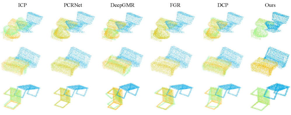
Unseen Objects. We train and test the models on the same categories. Training and testing datasets are clean and taken without any pretreatment. We apply a random transformation on the template point cloud to generate corresponding source point cloud . Table I(a) shows quantitative results of the various algorithms under current experimental settings, we observe that PCRDiffusion substantially outperforms all correspondence-free methods or correspondence-based methods in all metrics. Benefitting from the diffusion strategy, our method attains highly robust and accurate registration and improves the registration accuracy by an order of magnitude. In order to show the effect of our proposed approach clearly, a qualitative comparison of the registration results on correspondence-free method can be found in Figure 5. Our method ensure minimal impact on changing of the shape.
Unseen Categories. To verify the robustness of the categories, we evaluate PCRDiffusion by using different categories for training and testing. ModelNet40 is divided into two parts for training and testing, each consisting of 20 distinct categories. The testing portion comprises categories that were not present during training, thus ensuring that the model is evaluated on unseen data. Table I(b) shows the evaluation results of all models. To evaluate all algorithms fairly, the same categories and point clouds are used respectively in training and testing.
Gaussian Noise. We evaluate the performance in the presence of noise, which are always presented in real-world point clouds. We apply the random rigid transformation to the template point cloud, and randomly and independently jitter the points in the source point cloud and template point cloud by noises sampled from and clipped to on each axis. This experiment is significantly more challenging, because finding corresponding points will be more difficult, and the obvious one-to-one correspondence based coordinates will not exist. We retrain all models on the noisy data. As shown in Table I(c), our method outperforms other correspondence-free methods and correspondence-based methods.
4.3 PCRDiffusion for Partially Overlapping Scenarios
Inspired by Gaussian noise, we observe that our method performs well when corresponding relationship is found in the cluttered circumstances. Acquisition of partial point clouds is a common situation in the real-world, therefore we challenge a more extensive and difficult task. We crop the template point cloud and the source point cloud respectively, and retain 70% of the points. Noted that, the quantity of points in two point clouds is still consistent after cropping. Moreover, because the operation of cropping is random, some points in two point clouds may lose their correspondence. We verify quantitatively in Table I(d) and experimental results illustrate that our method can still achieve stable results comparing other methods, and the other baseline do not work well.
| Method | KITTI | 3DMatch | ||||||||||
| RMSE(R) | RMSE(t) | MAE(R) | MAE(t) | ERROR(R) | ERROR(t) | RMSE(R) | RMSE(t) | MAE(R) | MAE(t) | ERROR(R) | ERROR(t) | |
| ICP [37] | 18.9487 | 0.5466 | 12.6160 | 0.3563 | 20.6026 | 0.7752 | 25.4376 | 0.8635 | 13.9470 | 0.4202 | 25.7505 | 0.8614 |
| PointNetLK [9] | 7.0309 | 0.6846 | 0.8580 | 0.5257 | 1.4041 | 1.0589 | 2.1669 | 0.5779 | 0.3797 | 0.4792 | 0.6542 | 0.9653 |
| PCRNet [48] | 33.0369 | 6.8900 | 22.3317 | 5.4069 | 39.5509 | 10.7703 | 32.5824 | 1.3655 | 25.3004 | 1.0562 | 49.4726 | 2.1123 |
| DeepGMR [69] | 46.6050 | 0.4386 | 25.8622 | 0.2657 | 44.0679 | 0.5785 | 38.3840 | 1.2166 | 26.2025 | 0.8146 | 48.0517 | 1.6224 |
| FGR [68] | 13.9026 | 1.3483 | 1.7946 | 0.1454 | 3.2000 | 0.3053 | 1.5866 | 0.0810 | 0.2477 | 0.0099 | 0.4764 | 0.0200 |
| DCP [70] | 18.1473 | 10.7517 | 12.8834 | 7.4273 | 22.4225 | 16.3362 | 29.7272 | 1.2919 | 23.0550 | 0.9689 | 44.0671 | 1.9137 |
| FMR [10] | 7.5326 | 0.7692 | 1.4277 | 0.5663 | 2.2495 | 1.1334 | 3.3293 | 0.5690 | 0.6072 | 0.4712 | 1.0811 | 0.9423 |
| RPMNet [53] | 35.9824 | 0.7544 | 19.4641 | 0.3966 | 34.4617 | 0.8745 | 21.1454 | 0.4963 | 8.3353 | 0.2179 | 15.5514 | 0.4395 |
| PCRDiffusion | 0.6281 | 0.0209 | 0.3556 | 0.0129 | 0.8237 | 0.0282 | 0.1522 | 0.0061 | 0.1123 | 0.0040 | 0.2109 | 0.0081 |
4.4 Other Datasets
We conduct experiments on the real-world datasets: 3DMatch (indoor) [35] and KITTI odometry (outdoor) [36]. We utilize 3D object detection dateset in KITTI odometry consists of 14,999 outdoor driving scenarios scanned by Velodyne LiDAR and we use sequences 0-5 for training, 6-7 for validation and 8-10 for testing. 3DMatch dataset contains 62 indoor subscenes. Some subscenes represent the same scenario with different overlap rates, we ignore this characteristic and treat all subscenes as different scenes. For KITTI, the accuracy here refers to the accuracy of inter-frame matching for a single instance, rather than representing the accuracy of the odometry trajectory after matching all point clouds in the sequence.
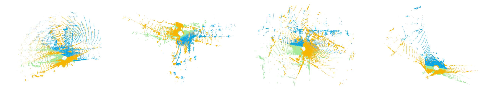
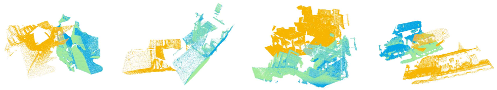
To be consistent with the input of ModelNet40, each input point cloud is randomly sampled to an average of 2,048 points. The other experimental settings are consistent with previous experiments. Fig. 6 and Fig. 7 show visualization results of KITTI and 3DMatch, respectively. As shown in Table II, we observe that PCRDiffusion can still achieve stable results comparing other methods. PCRDiffusion demonstrates remarkable generalization on real-world datasets, and this framework can still achieve optimal performance without the need for iterative processes.
4.5 Ablation Studies and Disscussion
We conduct extensive ablation studies for a better understanding of the various modules in PCRDiffusion framework. To achieve a fair comparison, we utilize the same experimental settings as Section 4.1 in ablation studies.
Diffusion or Diffsuion-Free? In order to validate the potential significance of the diffusion model in point cloud registration tasks, we conduct a series of ablation experiments. Specifically, we exclude the transformation encoder. The experimental outcomes are presented in Table III. We can observe that the model without diffusion has a clear performance drop, as they do not have refinement property given by diffusion model.
In addition, we have uncovered another intriguing characteristic. Upon removing the transformation encoder, our two proposed simplified frameworks degrade to the original iterative-free PCRNet and RPMNet. Remarkably, under the same iterative-free conditions, the utilization of the diffusion model yields substantial performance enhancement. This presents a highly promising practical avenue: integrating the diffusion model as a plug-and-play component into existing point cloud registration networks can yield exceptionally prominent results!
| Method | MAE(R) | MAE(t) | ERROR(R) | ERROR(t) |
| (a) w/ diffusion (CF) | 81.5854 | 0.4052 | 168.0197 | 0.7960 |
| (b) w/ diffusion (CB) | 6.3867 | 0.0698 | 12.7412 | 0.1429 |
| (c) PCRDiffusion (CF) | 1.6861 | 0.0216 | 3.2786 | 0.0448 |
| (d) PCRDiffusion (CB) | 0.7244 | 0.0153 | 1.2732 | 0.0318 |
Any Other Diffusion Objects? In our work, PCRDiffusion directly predicts object transformation from a random transformation. Furthermore, we unify the diffusion transformation object G to 7-dimensional vector (composed of a rotation quaternion and a translation). A natural idea arises: Is it possible to employ other transformation representation as diffusion object? We conduct experiments based on this notion, specifically, we replace the 7-dimensional vector into a 6-dimensional vector (composed of a rotation Euler angle and a translation), the distinction lies in the method of representing rotation. The experimental results are illustrated in Table IV. We can observe utilizing Euler angles does not yield performance enhancements, primarily due to the significant disparity in values between Euler angles and translation vectors. This incongruence introduces singularities into the linear noise processes for diffusion model.
| Method | MAE(R) | MAE(t) | ERROR(R) | ERROR(t) |
| 7-dimensional vectors | 0.7244 | 0.0153 | 1.2732 | 0.0318 |
| 6-dimensional vectors | 6.8240 | 0.0733 | 13.7542 | 0.1513 |
How to Fuse Noisy Transformation? During training, we construct noisy transformation by adding Gaussion noise, and feed it to transformation estimation decoder after encoding. In our work, we fuse the encoded noisy transformation features with the feature of source point cloud . Additionally, we have also explored two alternative approaches: (A) concatenating all features and (B) fuse with the feature of source point cloud . The experimental outcomes are illustrated in Table V. Practice proves that the model using approach A fails to converge and exhibits extreme instability. Furthermore, the fused approach demonstrates no significant variation in performance.
| Step | MAE(R) | MAE(t) | ERROR(R) | ERROR(t) |
| - | - | - | - | |
| 1.6887 | 0.0216 | 3.1686 | 0.0446 | |
| 1.6861 | 0.0216 | 3.2786 | 0.0448 |
Accuracy vs. Speed. We test the inference speed of PCRDiffusion in Table VI. The run time is evaluated on an NVIDIA RTX 3090 GPU with a mini-batch size of 1. The experimental results show that utilizing correspondence-based PCRDiffusion (PCRDiffusion CB) and correspondence-free PCRDiffusion (PCRDiffusion CF) respectively lead to the fastest inference speeds in all correspondence-based and correspondence-free methods. This is attributed to the iterative-free nature of our proposed framework, and it requires only a single step during reverse diffusion.
| Method | MAE(R) | MAE(t) | ERROR (R) | ERROR (t) | Time(s) |
| ICP () | 11.7468 | 0.1686 | 23.1548 | 0.3497 | 0.0042 |
| PointNetLK () | 1.7362 | 0.4907 | 4.0421 | 0.9741 | 0.7111 |
| PCRNet () | 10.2498 | 0.1168 | 19.0487 | 0.2442 | 1.2318 |
| DeepGMR () | 23.5162 | 0.3291 | 45.7786 | 0.6758 | 0.1053 |
| FGR () | 1.9971 | 0.0268 | 4.3337 | 0.0582 | 0.0916 |
| DCP () | 10.7846 | 0.1340 | 20.8744 | 0.2740 | 0.2819 |
| FMR () | 1.5962 | 0.4886 | 3.8090 | 0.9751 | 1.0472 |
| RPMNet () | 1.4399 | 0.0170 | 2.9619 | 0.0357 | 0.1626 |
| PCRDiffusion (CF) () | 1.6861 | 0.0216 | 3.2786 | 0.0448 | < |
| PCRDiffusion (CB) () | 0.7244 | 0.0153 | 1.2732 | 0.0318 | 0.0986 |
Sampling Steps. We conduct experiments employing diverse sampling steps on correspondence-free method. The results are shown in Table VII. The results of these experiments indicate that PCRDiffusion yields optimal outcomes within a single step, and as the number of sampling iterations increases, performance rapidly converges to stability.
| Steps | MAE(R) | MAE(t) | ERROR(R) | ERROR(t) |
| 1 | 1.6861 | 0.0216 | 3.2786 | 0.0448 |
| 2 | 1.6625 | 0.0215 | 3.1962 | 0.0445 |
| 4 | 1.6625 | 0.0215 | 3.1962 | 0.0445 |
| 8 | 1.6625 | 0.0215 | 3.1962 | 0.0445 |
5 Conclusion
In this work, we propose a novel point cloud registration paradigm, PCRDiffsuion, by viewing object transformation as a denoising diffusion process from noisy transformation to object transformation. Our ”noise-to-ground truth transformation” pipeline has several appealing advantage of Once-for-All: (i) We train the network only once, and no iteration strategy is required to update source point cloud during training and inference. (ii) We can adjust the number of denoising sampling steps to improve the registration accuracy or accelerate the inference speed. PCRDiffusion achieves favorable performance compared to well-established point cloud registration methods.
To further explore the potential of diffusion model to solve point cloud registartion tasks, several future works are beneficial. An attempt is to apply PCRDiffusion to multimodel tasks, for example, utilizing the image as the condition to guide point cloud registration.
References
- [1] H. Guo, J. Zhu, and Y. Chen, “E-loam: Lidar odometry and mapping with expanded local structural information,” IEEE Transactions on Intelligent Vehicles, vol. 8, no. 2, pp. 1911–1921, 2023.
- [2] J. Engel, J. Stückler, and D. Cremers, “Large-scale direct slam with stereo cameras,” in IEEE/RSJ International Conference on Intelligent Robots and Systems, 2015, pp. 1935–1942.
- [3] H. Guo, S. Peng, H. Lin, Q. Wang, G. Zhang, H. Bao, and X. Zhou, “Neural 3d scene reconstruction with the manhattan-world assumption,” in Proceedings of the IEEE/CVF Conference on Computer Vision and Pattern Recognition, 2022, pp. 5511–5520.
- [4] Y. Siddiqui, J. Thies, F. Ma, Q. Shan, M. Nießner, and A. Dai, “Retrievalfuse: Neural 3d scene reconstruction with a database,” in Proceedings of the IEEE/CVF International Conference on Computer Vision, 2021, pp. 12 568–12 577.
- [5] J. Sun, Z. Wang, S. Zhang, X. He, H. Zhao, G. Zhang, and X. Zhou, “Onepose: One-shot object pose estimation without cad models,” in Proceedings of the IEEE/CVF Conference on Computer Vision and Pattern Recognition, 2022, pp. 6825–6834.
- [6] T. Lee, B.-U. Lee, I. Shin, J. Choe, U. Shin, I. S. Kweon, and K.-J. Yoon, “Uda-cope: unsupervised domain adaptation for category-level object pose estimation,” in Proceedings of the IEEE/CVF Conference on Computer Vision and Pattern Recognition, 2022, pp. 14 891–14 900.
- [7] Z. Zhu, S. Peng, V. Larsson, W. Xu, H. Bao, Z. Cui, M. R. Oswald, and M. Pollefeys, “Nice-slam: Neural implicit scalable encoding for slam,” in Proceedings of the IEEE/CVF Conference on Computer Vision and Pattern Recognition, 2022, pp. 12 786–12 796.
- [8] Y. Fan, Q. Zhang, Y. Tang, S. Liu, and H. Han, “Blitz-slam: A semantic slam in dynamic environments,” Pattern Recognition, vol. 121, p. 108225, 2022.
- [9] Y. Aoki, H. Goforth, R. A. Srivatsan, and S. Lucey, “Pointnetlk: Robust & efficient point cloud registration using pointnet,” in Proceedings of the IEEE/CVF Conference on Computer Vision and Pattern Recognition, 2019, pp. 7163–7172.
- [10] X. Huang, G. Mei, and J. Zhang, “Feature-metric registration: A fast semi-supervised approach for robust point cloud registration without correspondences,” in Proceedings of the IEEE/CVF Conference on Computer Vision and Pattern Recognition, 2020, pp. 11 366–11 374.
- [11] G. Mei, “Point cloud registration with self-supervised feature learning and beam search,” in Digital Image Computing: Techniques and Applications. IEEE, 2021, pp. 01–08.
- [12] G. Mei, X. Huang, J. Zhang, and Q. Wu, “Partial point cloud registration via soft segmentation,” in IEEE International Conference on Image Processing. IEEE, 2022, pp. 681–685.
- [13] H. Xu, S. Liu, G. Wang, G. Liu, and B. Zeng, “Omnet: Learning overlapping mask for partial-to-partial point cloud registration,” in Proceedings of the IEEE/CVF International Conference on Computer Vision, 2021, pp. 3132–3141.
- [14] X. Bai, Z. Luo, L. Zhou, H. Chen, L. Li, Z. Hu, H. Fu, and C.-L. Tai, “Pointdsc: Robust point cloud registration using deep spatial consistency,” in Proceedings of the IEEE/CVF Conference on Computer Vision and Pattern Recognition, 2021, pp. 15 859–15 869.
- [15] C. Choy, W. Dong, and V. Koltun, “Deep global registration,” in Proceedings of the IEEE/CVF Conference on Computer Vision and Pattern Recognition, 2020, pp. 2514–2523.
- [16] S. Huang, Z. Gojcic, M. Usvyatsov, A. Wieser, and K. Schindler, “Predator: Registration of 3d point clouds with low overlap,” in Proceedings of the IEEE/CVF Conference on Computer Vision and Pattern Recognition, 2021, pp. 4267–4276.
- [17] Z. J. Yew and G. H. Lee, “Regtr: End-to-end point cloud correspondences with transformers,” in Proceedings of the IEEE/CVF Conference on Computer Vision and Pattern Recognition, 2022, pp. 6677–6686.
- [18] J. Ho, A. Jain, and P. Abbeel, “Denoising diffusion probabilistic models,” Advances in Neural Information Processing Systems, vol. 33, pp. 6840–6851, 2020.
- [19] J. Austin, D. D. Johnson, J. Ho, D. Tarlow, and R. van den Berg, “Structured denoising diffusion models in discrete state-spaces,” Advances in Neural Information Processing Systems, vol. 34, pp. 17 981–17 993, 2021.
- [20] O. Avrahami, D. Lischinski, and O. Fried, “Blended diffusion for text-driven editing of natural images,” in Proceedings of the IEEE/CVF Conference on Computer Vision and Pattern Recognition, 2022, pp. 18 208–18 218.
- [21] L. Zhou, Y. Du, and J. Wu, “3d shape generation and completion through point-voxel diffusion,” in Proceedings of the IEEE/CVF International Conference on Computer Vision, 2021, pp. 5826–5835.
- [22] Z. Lyu, Z. Kong, X. Xu, L. Pan, and D. Lin, “A conditional point diffusion-refinement paradigm for 3d point cloud completion,” arXiv preprint arXiv:2112.03530, 2021.
- [23] T. Amit, T. Shaharbany, E. Nachmani, and L. Wolf, “Segdiff: Image segmentation with diffusion probabilistic models,” arXiv preprint arXiv:2112.00390, 2021.
- [24] D. Baranchuk, I. Rubachev, A. Voynov, V. Khrulkov, and A. Babenko, “Label-efficient semantic segmentation with diffusion models,” arXiv preprint arXiv:2112.03126, 2021.
- [25] E. A. Brempong, S. Kornblith, T. Chen, N. Parmar, M. Minderer, and M. Norouzi, “Denoising pretraining for semantic segmentation,” in Proceedings of the IEEE/CVF Conference on Computer Vision and Pattern Recognition, 2022, pp. 4175–4186.
- [26] T. Chen, L. Li, S. Saxena, G. Hinton, and D. J. Fleet, “A generalist framework for panoptic segmentation of images and videos,” arXiv preprint arXiv:2210.06366, 2022.
- [27] A. Graikos, N. Malkin, N. Jojic, and D. Samaras, “Diffusion models as plug-and-play priors,” arXiv preprint arXiv:2206.09012, 2022.
- [28] B. Kim, Y. Oh, and J. C. Ye, “Diffusion adversarial representation learning for self-supervised vessel segmentation,” arXiv preprint arXiv:2209.14566, 2022.
- [29] J. Wolleb, R. Sandkühler, F. Bieder, P. Valmaggia, and P. C. Cattin, “Diffusion models for implicit image segmentation ensembles,” in International Conference on Medical Imaging with Deep Learning. PMLR, 2022, pp. 1336–1348.
- [30] J. Sohl-Dickstein, E. Weiss, N. Maheswaranathan, and S. Ganguli, “Deep unsupervised learning using nonequilibrium thermodynamics,” in International Conference on Machine Learning. PMLR, 2015, pp. 2256–2265.
- [31] C. R. Qi, H. Su, K. Mo, and L. J. Guibas, “Pointnet: Deep learning on point sets for 3d classification and segmentation,” in Proceedings of the IEEE/CVF Conference on Computer Vision and Pattern Recognition, 2017, pp. 652–660.
- [32] Y. Wang, Y. Sun, Z. Liu, S. E. Sarma, M. M. Bronstein, and J. M. Solomon, “Dynamic graph cnn for learning on point clouds,” ACM Transactions On Graphics, vol. 38, no. 5, pp. 1–12, 2019.
- [33] C. R. Qi, L. Yi, H. Su, and L. J. Guibas, “Pointnet++: Deep hierarchical feature learning on point sets in a metric space,” Advances in Neural Information Processing Systems, vol. 30, 2017.
- [34] Z. Wu, S. Song, A. Khosla, F. Yu, L. Zhang, X. Tang, and J. Xiao, “3d shapenets: A deep representation for volumetric shapes,” in Proceedings of the IEEE/CVF Conference on Computer Vision and Pattern Recognition, 2015, pp. 1912–1920.
- [35] A. Zeng, S. Song, M. Nießner, M. Fisher, J. Xiao, and T. Funkhouser, “3dmatch: Learning local geometric descriptors from rgb-d reconstructions,” in Proceedings of the IEEE/CVF Conference on Computer Vision and Pattern Recognition, 2017, pp. 1802–1811.
- [36] A. Geiger, P. Lenz, and R. Urtasun, “Are we ready for autonomous driving? the kitti vision benchmark suite,” in Proceedings of the IEEE/CVF Conference on Computer Vision and Pattern Recognition, 2012, pp. 3354–3361.
- [37] P. J. Besl and N. D. McKay, “Method for registration of 3-d shapes,” in Sensor fusion IV: Control Paradigms and Data Structures, 1992, pp. 586–606.
- [38] A. Kurobe, Y. Sekikawa, K. Ishikawa, and H. Saito, “Corsnet: 3d point cloud registration by deep neural network,” IEEE Robotics and Automation Letters, vol. 5, no. 3, pp. 3960–3966, 2020.
- [39] A. Segal, D. Haehnel, and S. Thrun, “Generalized-icp.” in Robotics: Science and Systems, 2009.
- [40] J. Yang, H. Li, D. Campbell, and Y. Jia, “Go-icp: A globally optimal solution to 3d icp point-set registration,” IEEE Transactions on Pattern Analysis and Machine Intelligence, vol. 38, no. 11, pp. 2241–2254, 2015.
- [41] S. Bouaziz, A. Tagliasacchi, and M. Pauly, “Sparse iterative closest point,” in Computer Graphics Forum, 2013, pp. 113–123.
- [42] A. W. Fitzgibbon, “Robust registration of 2d and 3d point sets,” Image and Vision Computing, vol. 21, no. 13-14, pp. 1145–1153, 2003.
- [43] S. Rusinkiewicz, “A symmetric objective function for icp,” ACM Transactions on Graphics, vol. 38, no. 4, pp. 1–7, 2019.
- [44] B. Bellekens, V. Spruyt, R. Berkvens, R. Penne, and M. Weyn, “A benchmark survey of rigid 3d point cloud registration algorithms,” in Proceedings of International Conference on Ambient Computing, Applications, Services and Technologies, 2015, pp. 118–127.
- [45] S. Du, G. Xu, S. Zhang, X. Zhang, Y. Gao, and B. Chen, “Robust rigid registration algorithm based on pointwise correspondence and correntropy,” Pattern Recognition Letters, vol. 132, pp. 91–98, 2020.
- [46] D. Chetverikov, D. Svirko, D. Stepanov, and P. Krsek, “The trimmed iterative closest point algorithm,” in International Conference on Pattern Recognition, vol. 3, 2002, pp. 545–548.
- [47] S. Rusinkiewicz and M. Levoy, “Efficient variants of the icp algorithm,” in Proceedings of International Conference on 3-D Digital Imaging and Modeling, 2001, pp. 145–152.
- [48] V. Sarode, X. Li, H. Goforth, Y. Aoki, R. A. Srivatsan, S. Lucey, and H. Choset, “Pcrnet: Point cloud registration network using pointnet encoding,” arXiv preprint arXiv:1908.07906, 2019.
- [49] J. Li, C. Zhang, Z. Xu, H. Zhou, and C. Zhang, “Iterative distance-aware similarity matrix convolution with mutual-supervised point elimination for efficient point cloud registration,” in European Conference on Computer Vision, 2020, pp. 378–394.
- [50] Y. Yuan, Y. Wu, X. Fan, M. Gong, W. Ma, and Q. Miao, “Egst: Enhanced geometric structure transformer for point cloud registration,” IEEE Transactions on Visualization & Computer Graphics, no. 01, pp. 1–13, 2023.
- [51] Z. Dang, F. Wang, and M. Salzmann, “Learning 3d-3d correspondences for one-shot partial-to-partial registration,” arXiv preprint arXiv:2006.04523, 2020.
- [52] M. Cuturi, “Sinkhorn distances: Lightspeed computation of optimal transport,” Advances in Neural Information Processing Systems, vol. 26, 2013.
- [53] Z. J. Yew and G. H. Lee, “Rpm-net: Robust point matching using learned features,” in Proceedings of the IEEE/CVF Conference on Computer Vision and Pattern Recognition, 2020, pp. 11 824–11 833.
- [54] H. Deng, T. Birdal, and S. Ilic, “Ppfnet: Global context aware local features for robust 3d point matching,” in Proceedings of the IEEE conference on computer vision and pattern recognition, 2018, pp. 195–205.
- [55] Y. Song and S. Ermon, “Generative modeling by estimating gradients of the data distribution,” Advances in Neural Information Processing Systems, vol. 32, 2019.
- [56] Y. Song, J. Sohl-Dickstein, D. P. Kingma, A. Kumar, S. Ermon, and B. Poole, “Score-based generative modeling through stochastic differential equations,” arXiv preprint arXiv:2011.13456, 2020.
- [57] I. Goodfellow, J. Pouget-Abadie, M. Mirza, B. Xu, D. Warde-Farley, S. Ozair, A. Courville, and Y. Bengio, “Generative adversarial networks,” Communications of the ACM, vol. 63, no. 11, pp. 139–144, 2020.
- [58] P. Dhariwal and A. Nichol, “Diffusion models beat gans on image synthesis,” Advances in Neural Information Processing Systems, vol. 34, pp. 8780–8794, 2021.
- [59] E. Mathieu and M. Nickel, “Riemannian continuous normalizing flows,” Advances in Neural Information Processing Systems, vol. 33, pp. 2503–2515, 2020.
- [60] S. Luo and W. Hu, “Diffusion probabilistic models for 3d point cloud generation,” in Proceedings of the IEEE/CVF Conference on Computer Vision and Pattern Recognition, 2021, pp. 2837–2845.
- [61] ——, “Score-based point cloud denoising,” in Proceedings of the IEEE/CVF International Conference on Computer Vision, 2021, pp. 4583–4592.
- [62] A. Vahdat, F. Williams, Z. Gojcic, O. Litany, S. Fidler, K. Kreis et al., “Lion: Latent point diffusion models for 3d shape generation,” Advances in Neural Information Processing Systems, vol. 35, pp. 10 021–10 039, 2022.
- [63] S. Chen, P. Sun, Y. Song, and P. Luo, “Diffusiondet: Diffusion model for object detection,” arXiv preprint arXiv:2211.09788, 2022.
- [64] D. P. Kingma and M. Welling, “Auto-encoding variational bayes,” arXiv preprint arXiv:1312.6114, 2013.
- [65] A. Q. Nichol and P. Dhariwal, “Improved denoising diffusion probabilistic models,” in International Conference on Machine Learning. PMLR, 2021, pp. 8162–8171.
- [66] D. E. Rumelhart, G. E. Hinton, and R. J. Williams, “Learning representations by back-propagating errors,” nature, vol. 323, no. 6088, pp. 533–536, 1986.
- [67] D. P. Kingma and J. Ba, “Adam: A method for stochastic optimization,” arXiv preprint arXiv:1412.6980, 2014.
- [68] Q.-Y. Zhou, J. Park, and V. Koltun, “Fast global registration,” in European Conference on Computer Vision, 2016, pp. 766–782.
- [69] W. Yuan, B. Eckart, K. Kim, V. Jampani, D. Fox, and J. Kautz, “Deepgmr: Learning latent gaussian mixture models for registration,” in European Conference on Computer Vision, 2020, pp. 733–750.
- [70] Y. Wang and J. M. Solomon, “Deep closest point: Learning representations for point cloud registration,” in Proceedings of the IEEE/CVF International Conference on Computer Vision, 2019, pp. 3523–3532.
- [71] Q.-Y. Zhou, J. Park, and V. Koltun, “Open3d: A modern library for 3d data processing,” arXiv preprint arXiv:1801.09847, 2018.
![[Uncaptioned image]](https://cdn.awesomepapers.org/papers/936622e5-00e0-4a5d-9261-90282fddefdc/WuYue.jpg) |
Yue Wu received the B.Eng. and Ph.D. degrees from Xidian University, Xi’an, China, in 2011 and 2016, respectively. Since 2016, he has been a Teacher with Xidian University. He is currently an Associate Professor with Xidian University. He has authored or co-authored more than 70 papers in refereed journals and proceedings. His research interests include computational intelligence and its Applications. He is the Secretary General of Chinese Association for Artificial Intelligence-Youth Branch, Chair of CCF YOCSEF Xi’an, Senior Member of Chinese Computer Federation. He is Editorial Board Member for over five journals, including Remote Sensing, Applied Sciences, Electronics, Mathematics. |
![[Uncaptioned image]](https://cdn.awesomepapers.org/papers/936622e5-00e0-4a5d-9261-90282fddefdc/YuanYongzhe.jpg) |
Yongzhe Yuan is currently pursuing the Ph.D degree with the School of Computer Science and Technology, the Key Laboratory of Collaborative Intelligence Systems of Ministry of Education, Xidian University, Xi’an. His research interests include deep learning, 3D computer vision and remote sensing image understanding. |
![[Uncaptioned image]](https://cdn.awesomepapers.org/papers/936622e5-00e0-4a5d-9261-90282fddefdc/FanXiaolong.jpg) |
Xiaolong Fan received the B.S. degree from Northwest University, Xi’an, China, in 2016. He is currently pursuing the Ph.D. degree in pattern recognition and intelligent systems with the School of Electronic Engineering, the Key Laboratory of Intelligent Perception and Image Understanding of Ministry of Education of China, Xidian University, Xi’an. His research interests include deep neural network, graph representation learning, and computer vision. |
![[Uncaptioned image]](https://cdn.awesomepapers.org/papers/936622e5-00e0-4a5d-9261-90282fddefdc/GongMG.jpg) |
Maoguo Gong received the B.Eng. and Ph.D. degrees from Xidian University, Xi’an, China, in 2003 and 2009, respectively. Since 2006, he has been a Teacher with Xidian University. He was promoted to an Associate Professor and a Full Professor, in 2008 and 2010, respectively, with exceptive admission. He has authored or coauthored over 100 articles in journals and conferences. He holds over 20 granted patents as the first inventor. He is leading or has completed over twenty projects as the Principle Investigator, funded by the National Natural Science Foundation of China, the National Key Research and Development Program of China, and others. His research interests are broadly in the area of computational intelligence, with applications to optimization, learning, data mining, and image understanding. Prof. Gong is the Executive Committee Member of Chinese Association for Artificial Intelligence and a Senior Member of Chinese Computer Federation. He was the recipient of the prestigious National Program for Support of the Leading Innovative Talents from the Central Organization Department of China, the Leading Innovative Talent in the Science and Technology from the Ministry of Science and Technology of China, the Excellent Young Scientist Foundation from the National Natural Science Foundation of China, the New Century Excellent Talent from the Ministry of Education of China, and the National Natural Science Award of China. He is an Associate Editor or an Editorial Board Member for over five journals including the IEEE TRANSACTIONS ON EVOLUTIONARY COMPUTATION and the IEEE TRANSACTIONS ON NEURAL NETWORKS AND LEARNING SYSTEMS. |
![[Uncaptioned image]](https://cdn.awesomepapers.org/papers/936622e5-00e0-4a5d-9261-90282fddefdc/MiaoQG.jpg) |
Qiguang Miao received the M.Eng. and Ph.D. degrees in computer science from Xidian University, Xi’an, China, in 1996 and 2005, respectively. He is currently a Professor with the School of Computer Science and Technology, Xidian University. His research interests include intelligent image processing and multiscale geometric representations for images. |