PatchComplete: Learning Multi-Resolution Patch Priors for 3D Shape Completion on Unseen Categories

Understanding how to reconstruct 3D shapes is an essential task for 3D machine perception. In particular, the task of shape completion to predict a complete shape from partial input observations has been studied by various works toward understanding 3D shape structures. Recently, many works have leveraged deep learning techniques to learn strong data-driven priors for shape completion, focusing on various different representations, e.g. volumetric grids [45, 14], continuous implicit functions [31, 22, 30, 7, 40, 36, 37], point clouds [32], and meshes [12, 20, 34, 35]. These works tend to focus on strong synthetic supervision on a small set of train categories, achieving impressive performance on unseen shapes from train categories, but often struggling to generalize to unseen classes. We focus on learning more generalizable, local shape priors in order to effectively reconstruct complete shapes on unseen class categories.

Several works have been developed to tackle the challenging task of few-shot or zero-shot shape reconstruction, as observations in-the-wild often contain a wide diversity of objects. In the few-shot scenario where several examples of novel categories are available, Wallace and Hariharan [42] learn to refine a given category prior. Michalkiewicz et al. [23] further propose to learn compositional shape priors for single-view reconstruction.

In the zero-shot scenario without any examples seen for novel categories, Naeem et al. [25] learn priors from seen categories to generate segmentation masks for unseen categories. Zhang et al. [48] additionally proposed to use spherical map representations to learn priors for the reconstruction of novel categories. Thai et al. [39] recently developed an approach to transfer knowledge from an RGB image for shape reconstruction. We also tackle a zero-shot shape reconstruction task, by learning a multi-resolution set of strong local shape priors to compose a reconstructed shape.

Several recent works have explored learning shape priors by leveraging a VQ-VAE backbone with autoregressive prediction to perform shape reconstruction [24, 46]. In contrast, we propose to learn multi-resolution shape priors without requiring any sequence interpretation, which enables direct applicability to real-world scan data that often contains noise and clutter. Additionally, hierarchical reconstruction has shown promising results for shape reconstruction [2, 6]. Our approach also takes a multi-resolution perspective, but learns explicit shape and local patch priors and their correlation to input partial observations for robust shape completion.

Our method aims to learn effective 3D shape priors that enable general shape completion from partial input scan data, on novel class categories not seen during training. Key to our approach is the observation that 3D shapes often share repeated local patterns – for instance, chairs, tables, and nightstands all share a support surface, and chair or table legs can share a similar structure with lamp rods. Inspired by this, we regard a complete object as a set of substructures, where each substructure represents a local geometric region. We thus propose PatchComplete to learn such local priors and assemble them into a complete shape from a partial scan. An overview of our approach is shown in Figure 2.

We first learn local shape priors from ground-truth train objects. We represent both the input partial scan $\mathcal{S}$ and the ground-truth shape $\mathcal{G}$ as 3D truncated signed distance field grids of size $D^{3}$. Figure 3 illustrates the process of learning local shape priors. We learn to build mappings from local regions in incomplete input observations to local priors based on complete shapes, in order to robustly reconstruct the complete shape output.

We first aim to learn patch-based priors, which we extract from learnable global shape priors $\{\mathcal{T}^{c}\}$. We denote $\mathcal{G}^{c}$ as the set of ground-truth train objects in the $c$-th category. These $\{\mathcal{T}^{c}\}$ priors are initialized per train category $c$ based on mean-shift clustering within shapes in $\mathcal{G}^{c}$. Thus $\mathcal{T}^{c}$ is a set of representative samples in each category, which are encoded parallel to the input scan $\mathcal{S}$.

Both encoders are analogously structured as 3D convolutional encoders which spatially downsample by a factor of $R$, resulting in a 3D encoding of size $N^{3}$; $N=D/R$. The input encoding (from $\mathcal{S}$) are uniformly chunked into patches $\{\mathcal{Q}_{i}\}$, $i$=1,…,$N^{3}$; similarly, the encoded priors (from $\{\mathcal{T}^{c}\}$) are chunked into patches $\{\mathcal{K}^{c}_{i}\}$.

We then use each local part $\mathcal{Q}_{i}$ to query for the most informative encodings of complete local regions $\{\mathcal{K}^{c}_{i}\}$, building this mapping based on cross-attention [41]. Then for each input patch, we calculate its similarity with all local patches in representative shapes on training categories:

$$\mathrm{Attention}(\mathcal{Q}_{i},\mathcal{K})=\mathrm{softmax}(\frac{\mathcal{Q}_{i}\cdot{\mathcal{K}}^{T}}{d/2}),\\ \mathcal{K}=\{\mathcal{K}^{c}_{i}|i=1,...,N^{3},c=1,...,C\},$$

(1)

where $d$ is the dimension of the encoded vectors of $\mathcal{Q}_{i},\mathcal{K}^{c}_{i}$; $C$ is the category number. We then reconstruct complete shape patches $\{\mathcal{P}_{i}\}$ by:

$$\mathcal{P}_{i}=\mathrm{Attention}(\mathcal{Q}_{i},\mathcal{K})\cdot\mathcal{V}$$

(2)

where $\mathcal{V}=\{\mathcal{V}^{c}_{i}\}$ is the set of $N^{3}$ chunks (of resolution $R$) from shapes in all categories $\{\mathcal{T}^{c}\}$, where each $\mathcal{V}^{c}_{i}$ is paired with $\mathcal{K}^{c}_{i}\in\mathcal{K}$. We can then recompose $\{\mathcal{P}_{i}\}$ to the predicted full shape $P$.

In Section 3, we learn to complete shapes in a single patch resolution $R$. Since local substructures may exist at various scales, we learn patch priors under varying resolutions, which we then use to decode a complete shape. We use three patch resolutions ($R$=4, 8, 32), for which we learn patch priors. This results in three pairs of trained {input encoder, prior encoder} (see Figure 3). Given a partial input scan $\mathcal{S}$, each pair outputs a set of 1) input patch features $\{\mathcal{Q}^{R}_{i}\}$, and 2) prior patch features $\mathcal{K}^{R}$, under the resolution of $R$=4, 8, 32. In this section, we decode a complete shape from these multi-resolution patch priors.

Since $\mathcal{K}^{R}$ stores the patch priors, we use it as the (key, value) term into an attention module, where each input patch feature $\mathcal{Q}^{R}_{i}$ is used to query for the most informative prior features in $\mathcal{K}^{R}$ under different resolutions, from which we complete partial patches in feature spaces with a multi-scale fashion. We formulate this process by

$$\mathcal{O}^{R}_{i}=\mathrm{Concat}\left[\mathcal{Q}^{R}_{i},\mathrm{Attention}(\mathcal{Q}^{R}_{i},\mathcal{K}^{R})\cdot\mathcal{K}^{R}\right],R=4,8,32,$$

(3)

where we concatenate input patch feature with the attention result to compensate information loss on observable regions. This outputs $\{\mathcal{O}^{R}_{i}\}$ as the intermediate feature of the $i$-th patch; $i=1,...,N_{R}^{3}$. $N_{R}$ denotes the number of patches under the resolution $R$; $N_{R}=D/R$. We recompose all generated patch features into a volume $\mathcal{O}^{R}=\{\mathcal{O}^{R}_{i}|i=1,...,N_{R}^{3}\}$. Note that the dimension of each grid feature in $\{\mathcal{Q}^{R}_{i}\}$ and $\mathcal{K}^{R}$ equals to $d$ (see Eq. 1). Then $\mathcal{O}^{R}$ is with the dimension of $N_{R}^{3}\times 2d$.

We then sequentially use 3D convolution decoders to upsample and concatenate $\mathcal{O}^{R}$ from low to high resolution to fuse all the shape features as in

$$\begin{split}\mathcal{O}^{R_{r+1}}&=\mathrm{Concat}\left[\mathrm{Upsample}(\mathcal{O}^{R_{r}}),\mathcal{O}^{R_{r+1}}\right],R_{r}|_{r=1,2,3}=32,8,4,\\ \mathcal{O}_{pred}&=\mathrm{Conv}(\mathrm{Upsample}(\mathcal{O}^{R_{3}})).\end{split}$$

(4)

In Eq. 4, $\mathcal{O}^{R_{r}}$ has a lower resolution than $\mathcal{O}^{R_{r+1}}$. We then use deconvolution layers to upsample $\mathcal{O}^{R_{r}}$ to match the resolution of $\mathcal{O}^{R_{r+1}}$, and then concatenate them together. We recursively fuse $\mathcal{O}^{R_{r}}$ into $\mathcal{O}^{R_{r+1}}$, which produces $\mathcal{O}^{R_{3}}$ as the final fusion result with the resolution of $(D/4)^{3}$. An extra upsampling followed by a convolution layer is adopted to upsample $\mathcal{O}^{R_{3}}$ into our shape prediction $\mathcal{O}_{pred}$ with the dimension of $D^{3}$.

In training the feature fusion, we fix all parameters from the {input encoder, prior encoder} under the three resolutions, since they are pre-trained on Section 3 and provide better-learned priors and attention maps under these strong constraints. The whole pipeline for this section can be found in Figure 4.

We use an $\ell_{1}$ loss to supervise the TSDF value regression. We weight the $\ell_{1}$ loss to penalize false predictions based on the predicted signs as Eq. 5 shows, which represents whether this voxel grid is occupied or not. It is also used in the loss function in Section 3.

$$\mathcal{L}=w_{occ}\ell_{1}(\mathcal{O}^{occ}_{pred},\mathcal{O}_{gt})+w_{empty}\ell_{1}(\mathcal{O}^{empty}_{pred},\mathcal{O}_{gt})+\ell_{1}(\mathcal{O}^{correct}_{pred},\mathcal{O}_{gt}).$$

(5)

In Eq. 5, $\mathcal{O}^{empty}_{pred}$ represents the false positive TSDF values, where the ground truth has negative signs and the prediction has positive signs, which in general indicates the missing predictions. $\mathcal{O}^{occ}_{pred}$ represents false negative TSDF values, where the ground truth has positive signs and the prediction has negative signs, which indicates extra predictions. $\mathcal{O}^{correct}_{pred}$ means those predicted TSDF values with the same signs as the ground-truth. During training, we choose the weight for false positive ($w_{empty}$) as 5, and the weight for false negative ($w_{occ}$) as 3.

We train our approach on a single NVIDIA A6000 GPU, using an Adam optimizer with batch size 32 for a synthetic dataset and batch size 16 for a real-world dataset, and an initial learning rate of 0.001. We train for 80 epochs until convergence, and then decrease the learning rate by half after epoch 50. We use the same settings for learning priors and the multi-resolution decoding, which train for 4 and 15.5 hours respectively. For additional network architecture details, we refer to the supplemental material.

Note that for training for real scan data, we first pre-train on synthetic data and then fine-tune only the input encoder. We use 112 shape priors in our method, which are clustered from 3202 train shapes, and represented as TSDFs with truncation of 2.5 voxels.

In Table 1, we evaluate our approach in comparison with prior arts on unseen class categories of synthetic ShapeNet [5] data. Our approach on learning attention-based correlation to learned local shape priors results in notably improved reconstruction performance, with coherent global and local structures, as shown in Figure 5. In Table 1, our work outperforms other baselines both instance-wise and category-wise. One of the key factors is that our method learns multi-scale patch information from seen categories to complete unseen categories with enough flexibility, while most of the other baselines are designed for 3D shape completion on known categories, which hardly leverage shape priors across categories.

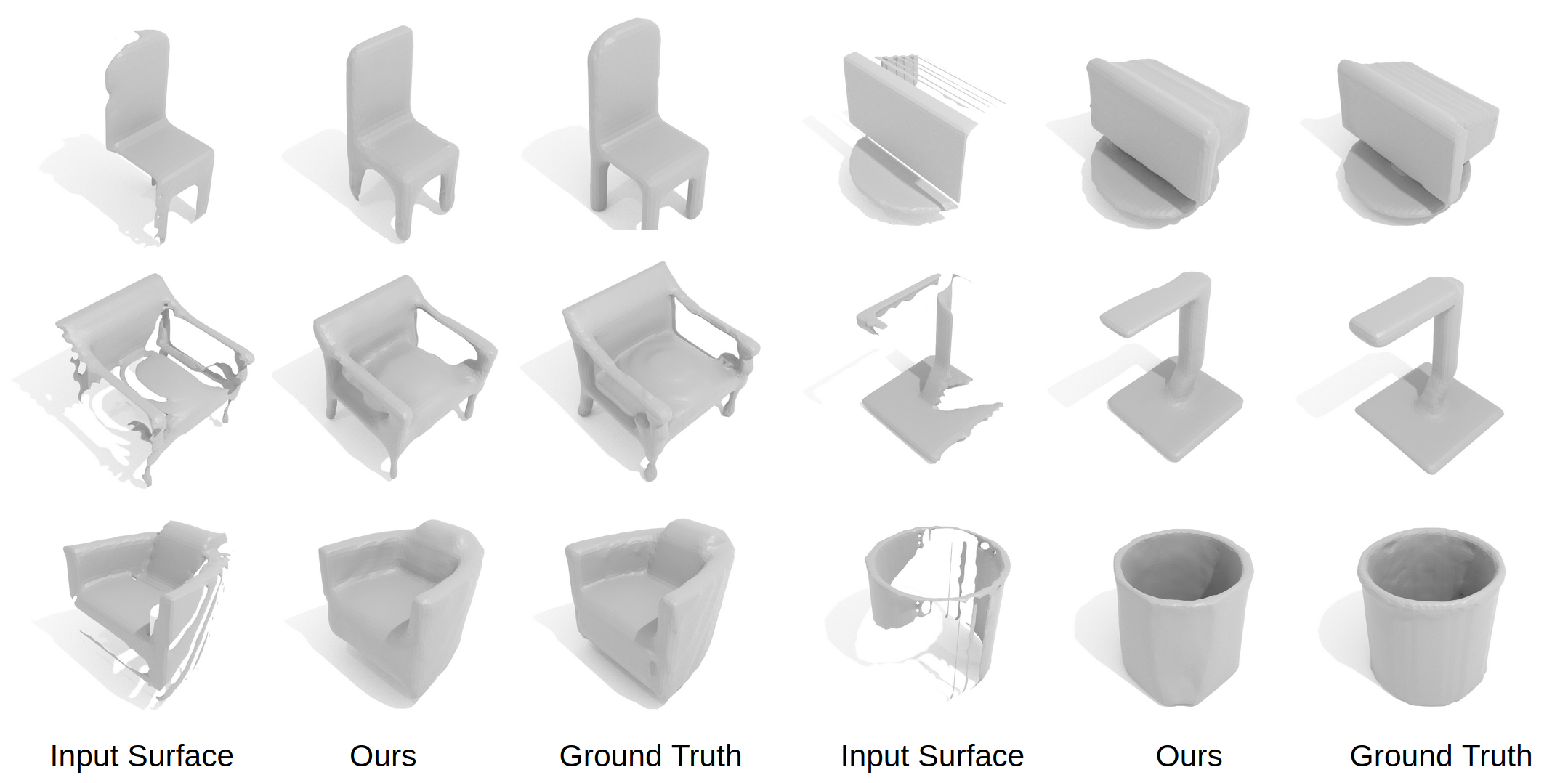
Table 2 evaluates our approach in comparison with prior arts on real scanned objects from unseen categories in ScanNet [11]. Here, input scans are not only partial but often contain noise and clutter; our multi-resolution learned priors enable more robust shape completion in this challenging scenario. Results in Figure 6 further demonstrate that our approach presents more coherent shape completion than prior methods by using cross-attention with learnable priors, which better preserves the global structures in coarse and cluttered environments.

While PatchComplete has presented a promising step towards learning more generalizable shape priors, various limitations remain. For instance, output shape completion is limited by the dense voxel grid resolution in representing fine-scale geometric details. Additionally, detected object bounding boxes are required for real scan data as input to independent shape completion predictions, while formulation considering other objects in the scene or an end-to-end framework could learn more effectively from global scene contextual information.

References

- [1] Avetisyan, A., Dahnert, M., Dai, A., Savva, M., Chang, A.X., Nießner, M.: Scan2cad: Learning cad model alignment in rgb-d scans (2018)
- [2] Bechtold, J., Tatarchenko, M., Fischer, V., Brox, T.: Fostering generalization in single-view 3d reconstruction by learning a hierarchy of local and global shape priors (2021)
- [3] Chabra, R., Lenssen, J.E., Ilg, E., Schmidt, T., Straub, J., Lovegrove, S., Newcombe, R.: Deep local shapes: Learning local sdf priors for detailed 3d reconstruction. In: European Conference on Computer Vision. pp. 608–625. Springer (2020)
- [4] Chang, A.X., Dai, A., Funkhouser, T., Halber, M., Niessner, M., Savva, M., Song, S., Zeng, A., Zhang, Y.: Matterport3D: Learning from RGB-D data in indoor environments. International Conference on 3D Vision (3DV) (2017)
- [5] Chang, A.X., Funkhouser, T., Guibas, L., Hanrahan, P., Huang, Q., Li, Z., Savarese, S., Savva, M., Song, S., Su, H., Xiao, J., Yi, L., Yu, F.: Shapenet: An information-rich 3d model repository (2015)
- [6] Chen, Z., Zhang, Y., Genova, K., Fanello, S., Bouaziz, S., Haene, C., Du, R., Keskin, C., Funkhouser, T., Tang, D.: Multiresolution deep implicit functions for 3d shape representation (2021)
- [7] Chibane, J., Alldieck, T., Pons-Moll, G.: Implicit functions in feature space for 3d shape reconstruction and completion (2020)
- [8] Choi, S., Zhou, Q.Y., Koltun, V.: Robust reconstruction of indoor scenes. In: 2015 IEEE Conference on Computer Vision and Pattern Recognition (CVPR). pp. 5556–5565. IEEE (2015)
- [9] Choy, C.B., Xu, D., Gwak, J., Chen, K., Savarese, S.: 3d-r2n2: A unified approach for single and multi-view 3d object reconstruction. In: European conference on computer vision. pp. 628–644. Springer (2016)
- [10] Curless, B., Levoy, M.: A volumetric method for building complex models from range images. In: Proceedings of the 23rd annual conference on Computer graphics and interactive techniques. pp. 303–312 (1996)
- [11] Dai, A., Chang, A.X., Savva, M., Halber, M., Funkhouser, T., Nießner, M.: Scannet: Richly-annotated 3d reconstructions of indoor scenes (2017)
- [12] Dai, A., Nießner, M.: Scan2mesh: From unstructured range scans to 3d meshes. In: Proceedings of the IEEE/CVF Conference on Computer Vision and Pattern Recognition. pp. 5574–5583 (2019)
- [13] Dai, A., Nießner, M., Zollhöfer, M., Izadi, S., Theobalt, C.: Bundlefusion: Real-time globally consistent 3d reconstruction using on-the-fly surface reintegration. ACM Transactions on Graphics (TOG) 36(3), 24 (2017)
- [14] Dai, A., Qi, C.R., Nießner, M.: Shape completion using 3d-encoder-predictor cnns and shape synthesis (2017)
- [15] Deng, B., Lewis, J.P., Jeruzalski, T., Pons-Moll, G., Hinton, G., Norouzi, M., Tagliasacchi, A.: Nasa neural articulated shape approximation. In: European Conference on Computer Vision. pp. 612–628. Springer (2020)
- [16] Fan, H., Su, H., Guibas, L.J.: A point set generation network for 3d object reconstruction from a single image. In: Proceedings of the IEEE conference on computer vision and pattern recognition. pp. 605–613 (2017)
- [17] Genova, K., Cole, F., Sud, A., Sarna, A., Funkhouser, T.: Local deep implicit functions for 3d shape. In: Proceedings of the IEEE/CVF Conference on Computer Vision and Pattern Recognition. pp. 4857–4866 (2020)
- [18] Izadi, S., Kim, D., Hilliges, O., Molyneaux, D., Newcombe, R., Kohli, P., Shotton, J., Hodges, S., Freeman, D., Davison, A., et al.: Kinectfusion: real-time 3d reconstruction and interaction using a moving depth camera. In: Proceedings of the 24th annual ACM symposium on User interface software and technology. pp. 559–568. ACM (2011)
- [19] Jiang, C., Sud, A., Makadia, A., Huang, J., Nießner, M., Funkhouser, T., et al.: Local implicit grid representations for 3d scenes. In: Proceedings of the IEEE/CVF Conference on Computer Vision and Pattern Recognition. pp. 6001–6010 (2020)
- [20] Li, X., Liu, S., Kim, K., Mello, S.D., Jampani, V., Yang, M.H., Kautz, J.: Self-supervised single-view 3d reconstruction via semantic consistency. In: European Conference on Computer Vision. pp. 677–693. Springer (2020)
- [21] Lorensen, W.E., Cline, H.E.: Marching cubes: A high resolution 3d surface construction algorithm. ACM siggraph computer graphics 21(4), 163–169 (1987)
- [22] Mescheder, L., Oechsle, M., Niemeyer, M., Nowozin, S., Geiger, A.: Occupancy networks: Learning 3d reconstruction in function space (2019)
- [23] Michalkiewicz, M., Tsogkas, S., Parisot, S., Baktashmotlagh, M., Eriksson, A., Belilovsky, E.: Learning compositional shape priors for few-shot 3d reconstruction (2021)
- [24] Mittal, P., Cheng, Y.C., Singh, M., Tulsiani, S.: AutoSDF: Shape priors for 3d completion, reconstruction and generation. In: CVPR (2022)
- [25] Naeem, M.F., Örnek, E.P., Xian, Y., Gool, L.V., Tombari, F.: 3d compositional zero-shot learning with decompositional consensus (2021)
- [26] Newcombe, R.A., Izadi, S., Hilliges, O., Molyneaux, D., Kim, D., Davison, A.J., Kohi, P., Shotton, J., Hodges, S., Fitzgibbon, A.: Kinectfusion: Real-time dense surface mapping and tracking. In: Mixed and augmented reality (ISMAR), 2011 10th IEEE international symposium on. pp. 127–136. IEEE (2011)
- [27] Nie, Y., Lin, Y., Han, X., Guo, S., Chang, J., Cui, S., Zhang, J., et al.: Skeleton-bridged point completion: From global inference to local adjustment. Advances in Neural Information Processing Systems 33, 16119–16130 (2020)
- [28] Nie, Y., Lin, Y., Han, X., Guo, S., Chang, J., Cui, S., Zhang, J.: Skeleton-bridged point completion: From global inference to local adjustment. In: Larochelle, H., Ranzato, M., Hadsell, R., Balcan, M.F., Lin, H. (eds.) Advances in Neural Information Processing Systems. vol. 33, pp. 16119–16130. Curran Associates, Inc. (2020)
- [29] Nießner, M., Zollhöfer, M., Izadi, S., Stamminger, M.: Real-time 3d reconstruction at scale using voxel hashing. ACM Transactions on Graphics (TOG) (2013)
- [30] Park, J.J., Florence, P., Straub, J., Newcombe, R., Lovegrove, S.: Deepsdf: Learning continuous signed distance functions for shape representation (2019)
- [31] Peng, S., Niemeyer, M., Mescheder, L., Pollefeys, M., Geiger, A.: Convolutional occupancy networks (2020)
- [32] Stutz, D., Geiger, A.: Learning 3d shape completion under weak supervision. International Journal of Computer Vision 128(5), 1162–1181 (2020)
- [33] Takikawa, T., Litalien, J., Yin, K., Kreis, K., Loop, C., Nowrouzezahrai, D., Jacobson, A., McGuire, M., Fidler, S.: Neural geometric level of detail: Real-time rendering with implicit 3d shapes. In: Proceedings of the IEEE/CVF Conference on Computer Vision and Pattern Recognition. pp. 11358–11367 (2021)
- [34] Tang, J., Han, X., Pan, J., Jia, K., Tong, X.: A skeleton-bridged deep learning approach for generating meshes of complex topologies from single rgb images. In: Proceedings of the ieee/cvf conference on computer vision and pattern recognition. pp. 4541–4550 (2019)
- [35] Tang, J., Han, X., Tan, M., Tong, X., Jia, K.: Skeletonnet: A topology-preserving solution for learning mesh reconstruction of object surfaces from rgb images. IEEE transactions on pattern analysis and machine intelligence (2021)
- [36] Tang, J., Lei, J., Xu, D., Ma, F., Jia, K., Zhang, L.: Sa-convonet: Sign-agnostic optimization of convolutional occupancy networks. In: Proceedings of the IEEE/CVF International Conference on Computer Vision. pp. 6504–6513 (2021)
- [37] Tang, J., Xu, D., Jia, K., Zhang, L.: Learning parallel dense correspondence from spatio-temporal descriptors for efficient and robust 4d reconstruction. In: Proceedings of the IEEE/CVF Conference on Computer Vision and Pattern Recognition. pp. 6022–6031 (2021)
- [38] Tatarchenko, M., Dosovitskiy, A., Brox, T.: Octree generating networks: Efficient convolutional architectures for high-resolution 3d outputs. In: Proceedings of the IEEE international conference on computer vision. pp. 2088–2096 (2017)
- [39] Thai, A., Stojanov, S., Upadhya, V., Rehg, J.M.: 3d reconstruction of novel object shapes from single images (2021)
- [40] Tretschk, E., Tewari, A., Golyanik, V., Zollhöfer, M., Stoll, C., Theobalt, C.: Patchnets: Patch-based generalizable deep implicit 3d shape representations (2021)
- [41] Vaswani, A., Shazeer, N., Parmar, N., Uszkoreit, J., Jones, L., Gomez, A.N., Kaiser, Ł., Polosukhin, I.: Attention is all you need. Advances in neural information processing systems 30 (2017)
- [42] Wallace, B., Hariharan, B.: Few-shot generalization for single-image 3d reconstruction via priors (2019)
- [43] Wang, N., Zhang, Y., Li, Z., Fu, Y., Liu, W., Jiang, Y.G.: Pixel2mesh: Generating 3d mesh models from single rgb images. In: Proceedings of the European conference on computer vision (ECCV). pp. 52–67 (2018)
- [44] Whelan, T., Leutenegger, S., Salas-Moreno, R.F., Glocker, B., Davison, A.J.: Elasticfusion: Dense slam without a pose graph. Proc. Robotics: Science and Systems, Rome, Italy (2015)
- [45] Wu, Z., Song, S., Khosla, A., Yu, F., Zhang, L., Tang, X., Xiao, J.: 3d shapenets: A deep representation for volumetric shapes (2015)
- [46] Yan, X., Lin, L., Mitra, N.J., Lischinski, D., Cohen-Or, D., Huang, H.: Shapeformer: Transformer-based shape completion via sparse representation. arXiv preprint arXiv:2201.10326 (2022)
- [47] Yang, G., Huang, X., Hao, Z., Liu, M.Y., Belongie, S., Hariharan, B.: Pointflow: 3d point cloud generation with continuous normalizing flows. In: Proceedings of the IEEE/CVF International Conference on Computer Vision. pp. 4541–4550 (2019)
- [48] Zhang, X., Zhang, Z., Zhang, C., Tenenbaum, J.B., Freeman, W.T., Wu, J.: Learning to reconstruct shapes from unseen classes (2018)
Appendix
In this supplementary material, we describe the data generation (Sec. A), settings for baseline methods (Sec. B), evaluation of category-wise error bars on ShapeNet and ScanNet (Sec. C), evaluation on seen categories for all the methods on ScanNet (Sec. D), additional ablation studies (Sec. E), network parameters and specifications (Sec. F), and additional qualitative results (Sec. G).
Appendix A Data Generation
ShapeNet [5]
We use ShapeNet222The license can be found here: https://shapenet.org/, received permission after registration without personally identifiable information or offensive content to test our performance on synthetic data. In order to generate watertight meshes as ground truth, we first normalize ShapeNet CAD models, and render depth maps under 20 different viewpoints for each model. We then use volumetric fusion [10] to generate truncated signed distance fields (TSDFs) with truncation value as 2.5 voxel units. Finally, we choose 4 views of TSDF as the input, which mimic the partial scan in real data (e.g., ScanNet). The main idea can be referred to [28]333https://github.com/yinyunie/depth_renderer.
We split the training and testing object categories on ShapeNet as follows. The 18 training categories are table, chair, sofa, cabinet, clock, bookshelf, piano, microwave, stove, file cabinet, trash bin, bowl, display, keyboard, dishwasher, washing machine, pots, faucet, and guitar; and the 8 novel testing categories are bathtub, lamp, bed, bag, printer, laptop, bench, and basket.
ScanNet [11]
We use ScanNet444The license can be found here: https://github.com/ScanNet/ScanNet, filled out an agreement without personally identifiable information or offensive content to test our method on real-world data. The inputs are directly extracted from ScanNet scenes based on the bounding box annotations from Scan2CAD [1]555The license can be found here::https://github.com/skanti/Scan2CAD, filled out an agreement without personally identifiable information or offensive content. We keep their real scale and convert them to voxel grids with truncation value at 3 voxel units, and save their voxel size separately. These inputs could contain walls, floors, or other cluttered backgrounds, which are transformed to canonical space to be aligned with the ShapeNet model coordinate system. The ground-truths are the corresponding complete and watertight ShapeNet meshes based on Scan2CAD annotations, which are generated with the similar method as above.
We split the training and testing object categories on ScanNet as follows. The 8 training categories are chair, table, sofa, trash bin, cabinet, bookshelf, file cabinet, and monitor; and the 6 novel testing categories are bathtub, lamp, bed, bag, basket, and printer, and each category has more than 50 samples for testing.
Alternative Train Category Splits
Here are two new category splits for the last ablation study. For Category Split 1, the 8 novel testing categories are trash bin, bed, piano bench, chair, monitor, lamp, laptop, washing machine. For Category Split 2, the 8 novel testing categories are basket, bookshelf, bowl, cabinet, laptop, pot, sofa, stove.
Appendix B Baseline Comparisons
We use the authors’ original implementations and hyperparameters in all the baselines for fair comparisons.
3D-EPN [14]
3D-EPN is a two-stage network, which completes partial 3D scans first and then reconstructs the completed shapes to a higher resolution by retrieving priors from a category-wise shape pool. In our case, priors for novel categories are not accessible, thus, we only compare its 3D Encoder-Predictor Network (the 3D completion model) on our dataset.
Wallace and Hariharan [42] (Few-Shot)
This method uses a few-shot learning strategy for single view completion with averaged shape prior for each category. For a fair comparison with other works, we adapt it to a zero-shot learning mechanism here. We pre-compute the averaged shape priors for each training category; during training, we use two voxel encoder modules in parallel for the occupied voxel grids inputs and the averaged shape priors based on the input category; in the testing step, since we cannot provide shape priors for novel categories, we average shape prior from all the training categories, and use this averaged shape prior as input to the prior encoder module, along with the testing samples for shape completion.
IF-Net [7]
IF-Net can predict implicit shape representations conditioned on different input modalities. (e.g., voxels, point clouds). We use occupied surface voxel grids as inputs, and use point clouds sampled from watertight ShapeNet meshes as the ground-truths for training and testing. We also normalize the ground-truth meshes from the ScanNet dataset to sample points.
AutoSDF [24]
AutoSDF learns latent patch priors using VQ-VAE along with a transformer-based autoregressive model for 3D shape completion, and manually picks the unknown patches during testing. Following their settings, we apply their method by using ground-truth SDFs as the training data; during testing on the ShapeNet data, we choose the patches that have more than 400 voxel grids (each patch has voxel grids) with negative signs as the unknown patches (unseen parts) that need to be generated.
Note that since AutoSDF work focuses on multi-model shape completion and produces multiple output possibilities, we report the performance of only the best prediction among the nine given an oracle to indicate the best (highest IoU value with respect to ground truth).
Furthermore, as there are no absolutely unknown patches for ScanNet scans because of the cluttered environments, we use the pipeline of their single view reconstruction task. We first replace their ResNet in resnet2vq_model with three 3D encoders (the same as 3D-EPN encoders) to extract the encoding features of desired dimensions; then we train this modified model along with the pre-trained pvq_vae_model with partial ScanNet inputs; finally we test our partial ScanNet inputs along with all the pre-trained models: resnet2vq_model, pvq_vae_model, and rand_tf_model.
Appendix C Category-wise Evaluations with Error Bars