Partial stabilization of nonlinear systems along a given trajectory

Trajectory tracking is one of the fundamental control problems which has numerous applications in robotics and process engineering. A theoretical justification of tracking properties of control algorithms requires the stability analysis of the tracking error dynamics in a neighborhood of the reference curve. The stability proof can be straightforwardly achieved, e.g., if the linearized error dynamics is completely controllable. Tracking algorithms, based on the feedback linearization and flatness techniques, are shown to be highly efficient for various engineering models.

For kinematically redundant manipulating robots, the tracking problem can be effectively formulated in terms of a part of the state variables that characterize the control objective. This analogy creates a connection between pragmatically driven issues in the field of robotics and the notion of partial stability, a concept that was rigorously defined by A.M. Lyapunov and has been extensively explored by many researchers (see, e.g., [31, 14, 38, 39, 40, 4, 22, 34, 41, 17, 25, 35, 15, 13, 42, 1, 27] and references therein). Specifically, the paper [14] explored the connection between partial stability and full-variable stability in nonholonomic mechanical systems, offering conditions for achieving partial stability. Issues of partial stabilization in the context of Lagrangian systems were investigated in [32, 18]. Controllers that utilize passivity-based approaches for partial stabilization have been suggested in [24, 3, 37]. The issue of achieving partial stabilization in stochastic dynamical systems is addressed, e.g., in the papers [28, 36, 44].

The issue of achieving partial stabilization within a finite time frame for systems in chained-form and cascade configurations has been investigated, as illustrated in [16, 5, 7]. An analysis of more extensive categories of nonlinear control systems can be found in [13, 19]. The suggested adequate conditions for partial stability are based on the premise that the system allows for a Lyapunov function, with the time derivative that is negatively definite concerning a specific subset of variables.

In the paper [29], the motion planning problem for autonomous vehicles is considered within the framework of manoeuvre automata. In order to ensure the safety of paths in complex environments, it is required to estimate the reachable set of each manoeuvre. The proposed motion planning scenario is illustrated by a unicycle mode with two controls corresponding to the angular velocity and the translational acceleration. The analogy between the equations of motion of nonholonomic systems and underwater vehicles has been pointed out in [2], where driftless control-affine systems have been used to model the kinematics of an autonomous submarine. These equations have been analyzed in the paper [10] in the context of trajectory tracking problem with oscillating inputs. A survey of recent advances in the motion planning of autonomous underwater vehicles (AUV) is presented in [26]. A mathematical model of an unmanned surface vehicle (USV) in the form of a nonlinear control-affine system with 6-dimensinal state and 3-dimensional force input is considered in [33]. For this dynamical model, a tracking controller is constructed under the assumption that the planar reference trajectory is regular enough and $C^{2}$-bounded. The stability proof of the tracking algorithm is based on Lyapunov’s direct method.

An important application of partial stability theory originates from planning the motion of robotic systems in task-spaces. The goal of the latter problem is to steer the output of a nonholonomic system to a neighborhood of the target point. As the number of output variables (which characterize the task space) is usually less than the dimension of the state space, this task fits into the framework of partial stabilization problems. An approach for solving the motion planning problem in task-space is proposed in [23] based on the Campbell–Baker–Hausdorff–Dynkin formula. The efficiency of this approach has been tested by the unicycle and car models with kinematic control. Fundamental solutions of the Laplace equation are exploited in [30] to generate obstacle-free motion of a disk robot in a bounded connected workspace. The control function, corresponding to the robot velocity, is obtained by an appropriate rescaling of the gradient of the potential function. The control scheme is implemented sequentially, and the convergence of the trajectories to the goal is proved. Computational complexity of the proposed control algorithm is estimated by numerical experiments.

While the field of partial stability theory has advanced substantially, contributions to the partial stabilization of underactuated nonlinear control systems remain relatively scarce. The challenge of partial stabilization persists for general nonholonomic systems due to the difficulty in formulating an appropriate Lyapunov-like function. In [9], practical conditions for partial asymptotic stability were introduced for control-affine systems that exhibit a partially asymptotically stable equilibrium in their averaged form. This paper tackles the issue of devising explicit partially stabilizing feedback mechanisms for nonlinear control-affine systems that comply with a specific Lie algebra rank condition in their vector fields.

This paper presents a novel approach to partial stabilization that significantly advances the state of the art by addressing the challenge of stabilizing along non-feasible curves – a task not previously tackled. By conceptualizing this problem through the lens of the stability of sets, we establish a unifies framework that allows for the stabilization of system behaviors in the vicinity of a given trajectory rather than at a fixed point. The introduction of time-varying feedback laws is a crucial point in our construction, ensuring exponential stability across a family of sets proximal to the non-feasible curve.

The rest of this paper is organized as follows. The partial stabilization problem is formulated in Section II within the framework of a family of sets. The main result (Theorem 1) is presented in Section III, and its proof is given in the Appendix. Section IV illustrates our control design scheme for an autonomous underwater vehicle model.

In this section, we consider the class of systems (4), whose control vector fields $g_{k}\in C^{1}(\mathbb{R}^{n};\mathbb{R}^{n_{1}})$ satisfy the following rank condition for all $x\in D$:

$$\text{ span}\left\{\big{(}g_{i}(x)\big{)}_{i\in S_{1}},\big{(}I_{n_{1}\times n}[f_{i_{1}},f_{i_{2}}](x)\big{)}_{(i_{1},i_{2})\in S_{2}}\right\}=\mathbb{R}^{n_{1}},$$

(5)

where $S_{1}$, $S_{2}$ are some sets of indices $S_{1}\subseteq\{1,2,...,m\},$ $S_{2}\subseteq\{1,2,...,m\}^{2}$ such that $|S_{1}|+|S_{2}|=n_{1}$.

This assumption represents a relaxation of the controllability rank condition that the vector fields of system (1) with their Lie brackets span the whole tangent space:

$$\text{ span}\left\{\big{(}f_{i}(x)\big{)}_{i\in\widetilde{S}_{1}},\big{(}[f_{i_{1}},f_{i_{2}}](x)\big{)}_{(i_{1},i_{2})\in\widetilde{S}_{2}}\right\}=\mathbb{R}^{n}$$

at each $x\in D$ with some $\widetilde{S}_{1}\subseteq\{1,2,...,m\},$ $\widetilde{S}_{2}\subseteq\{1,2,...,m\}^{2}$, $|\widetilde{S}_{1}|+|\widetilde{S}_{2}|=n$. For the partial stabilization problems, the latter requirement can be replaced with relaxed condition (5). Thus, we take into account only the first $n_{1}$ coordinates of $f_{i}(x)$ and $[f_{i_{1}},f_{i_{2}}](x)$, i.e. we exploit the vector fields $g_{i}(x)$ and $I_{n_{1}\times n}[f_{i_{1}},f_{i_{2}}](x)=\mathcal{L}_{f_{i_{1}}}(x)g_{i_{2}}(x)-\mathcal{L}_{f_{i_{2}}}(x)g_{i_{1}}(x)$. Consequently, a smaller set of vector fields is needed to satisfy the stabilizability condition, which simplifies the control design. Condition (5) has been proposed in [11] for the case $y^{*}(t)\equiv const,$ and we exploit it here for solving Problem 1.

In order to stabilize the $y$-variables of system (1) along a curve $y^{*}(t),$ we will use a time-varying feedback control of the form

	$\displaystyle u_{k}^{\varepsilon}(t,x,y^{*})=$	$\displaystyle\sum\limits_{i\in S_{1}}\phi_{i}^{k}(t,x,y^{*})$		(6)
		$\displaystyle+\frac{1}{\sqrt{\varepsilon}}\sum\limits_{(i_{1}i_{2})\in S_{2}}\phi_{i_{1},i_{2}}^{k}(t,x,y^{*}),k=\overline{1,m},$

where

		$\displaystyle\phi_{i}^{k}(t,x,y^{*})=\delta_{ki}a_{i}(x,y^{*}),$
		$\displaystyle\phi_{i_{1},i_{2}}^{k}(t,x,y^{*})=2\sqrt{\pi\kappa_{i_{1}i_{2}}|a_{i_{1}i_{2}}(x,y^{*})|}\left(\delta_{ki_{1}}\cos\left(\frac{2\pi\kappa_{i_{1}i_{2}}t}{\varepsilon}\right)\right.$
		$\displaystyle\qquad\qquad\left.+\delta_{ki_{2}}{\rm{sign}}(a_{i_{1}i_{2}}(x,y^{*}))\sin\left(\frac{2\pi\kappa_{i_{1}i_{2}}t}{\varepsilon}\right)\right).$

Here, $\varepsilon>0$ is a small parameter, $\kappa_{i_{1}i_{2}}\in\mathbb{N}$ are pairwise distinct numbers, $\delta_{ij}$ is the Kronecker delta, and $\left((a_{i}(x,y^{*}))_{i\in S_{1}},(a_{i_{1}i_{2}}(x,y^{*}))_{(i_{1}i_{2})\in S_{2}}\right)^{T}=a(x,y^{*}),$ where

$$a(x,y^{*})=-\alpha\mathcal{F}^{-1}(x)(y-y^{*}),\quad\alpha>0,$$

(7)

with $\mathcal{F}^{-1}(x)$ denoting the inverse for $n_{1}\times n_{1}$ matrix

$$\mathcal{F}(x)=\left((g_{i}(x))_{i\in S_{1}},(I_{n_{1}\times n}[f_{i_{1}},f_{i_{2}}](x))_{(i_{1}i_{2})\in S_{2}}\right).$$

Obviously, the matrix $\mathcal{F}(x)$ is nonsingular in $D$ because of condition (5).

Let us mention that controllers of the form (6)-(7) has been used, e.g. in [43, 9, 11]. In this paper, we adopt the control design from the above mentioned papers to solve Problem 1. Before formulating the main result of this section, we introduce several assumptions on the vector field of system (4) and the curve $y^{*}(t)$.

The following result shows that the family of controls (6)-(7) solves Problem 1 for system (4) under Assumption 1.

Theorem 1. Let Assumption 1 be satisfied for system (4) and a curve $y^{*}\in C(\mathbb{R}^{+};D_{y})$, and let $p,\delta>0$ be arbitrary numbers such that $B_{\delta}(\mathit{Y_{t}^{p}})\subset D$ for all $t\geq 0,$ where the sets $\mathit{Y_{t}^{p}}$ are defined in (3).

Then there exists an $\overline{\varepsilon}>0$ such that, for any $\varepsilon\in(0,\overline{\varepsilon}],$ the family of sets $\left\{\mathit{Y_{t}^{p}}\right\}_{t\geq 0}$ is asymptotically (and even exponentially) stable for system (4) with the controls $u_{k}=u_{k}^{\varepsilon}(t,x,y^{*})$ defined by (6) and the initial conditions $x(0)=x^{0}\in B_{\delta}(\mathit{Y_{t}^{p}}).$

The proof of this theorem is presented in the Appendix.

Consider the equations of motion of an autonomous underwater vehicle with four independent controls:

$$\begin{array}[]{lcl}\dot{x}_{1}=\cos(x_{5})\cos(x_{6})v,\\ \dot{x}_{2}=\cos(x_{5})\sin(x_{6})v,\\ \dot{x}_{3}=-\sin(x_{5})v,\\ \dot{x}_{4}=\omega_{1}+\omega_{2}\sin(x_{4})\tan(x_{5})+\omega_{3}\cos(x_{4})\tan(x_{5}),\\ \dot{x}_{5}=\omega_{2}\cos(x_{4})-\omega_{3}\sin(x_{4}),\\ \dot{x}_{6}=\omega_{2}\sin(x_{4})\sec(x_{5})+\omega_{3}\cos(x_{4})\sec(x_{5}).\end{array}$$

(8)

Here, $(x_{1},x_{2},x_{3})$ denote the position of the center of mass, $(x_{4},x_{5},x_{6})$ describe the vehicle orientation (Euler angles), $v$ is the translational velocity along the $Ox_{1}$ axis, and $\omega_{1},\omega_{2},\omega_{3}$ are the angular velocity components. Such equations of motion have been presented, e.g., in [2]. The stabilization problem for system (8) by means of oscillating control is considered in [9]. In this section, we consider the problem of stabilizing the $(x_{1},x_{2},x_{3})$ coordinates of system (8) by three controls $v$, $\omega_{2}$, and $\omega_{3}$, so we assume that the first component of the angular velocity cannot be controlled. Let us denote $v=u_{1},\omega_{2}=u_{2},\omega_{3}=u_{3},$ $y=(x_{1},x_{2},x_{3})^{T}$, $z=(x_{4},x_{5},x_{6})^{T}$, $x=(y^{T},z^{T})^{T}$, and rewrite system (8) in the form (4):

$\displaystyle\dot{y}=\sum_{k=1}^{3}u_{k}g_{k}(x),\;\dot{z}=h_{0}(t,x)+\sum_{k=1}^{3}u_{k}h_{k}(x),$

where

	$\displaystyle h_{0}(t,x)$	$\displaystyle=(\omega_{1}(t),0,0)^{T},$
	$\displaystyle g_{1}(x)$	$\displaystyle=(\cos x_{5}\cos x_{6},\cos x_{5}\sin x_{6},-\sin x_{5})^{T},$
	$\displaystyle g_{2}(x)$	$\displaystyle=g_{3}(x)=h_{1}(x)=(0,0,0)^{T},$
	$\displaystyle h_{2}(x)$	$\displaystyle=(\sin x_{4}\tan x_{5},\cos x_{4},\sin x_{4}\sec x_{5})^{T},$
	$\displaystyle h_{3}(x)$	$\displaystyle=(\cos x_{4}\tan x_{5},-\sin x_{4},\cos x_{4}\sec x_{5})^{T}.$

The rank condition (5) is satisfied in $D=\{x\in\mathbb{R}^{6}:-\frac{\pi}{2}<x_{5}<\frac{\pi}{2}\}$ with $S_{1}=\{1\},$ $S_{2}=\{(1,2),(1,3)\}.$ Indeed, it is easy to check that the matrix $\mathcal{F}(x)$ is nonsingular in $D$ with $\det\mathcal{F}(x)\equiv 1$:

$$\mathcal{F}(x)=\left(g_{1}(x)\quad I_{3\times 6}[f_{1},f_{2}](x)\quad I_{3\times 6}[f_{1},f_{3}](x)\right),$$

where

	$\displaystyle I_{3\times 6}$	$\displaystyle[f_{1},f_{2}](x)=\big{(}\cos x_{4}\sin x_{5}\cos x_{6}+\sin x_{4}\sin x_{6},$
		$\displaystyle\cos x_{4}\sin x_{5}\sin x_{6}-\sin x_{4}\cos x_{6},\,\cos x_{4}\cos x_{5}\big{)}^{T},$
	$\displaystyle I_{3\times 6}$	$\displaystyle[f_{1},f_{3}](x)=\big{(}-\sin x_{4}\sin x_{5}\cos x_{6}+\cos x_{4}\sin x_{6},$
		$\displaystyle-\sin x_{4}\sin x_{5}\sin x_{6}-\cos x_{4}\cos x_{6},\,-\sin x_{4}\cos x_{5}\big{)}^{T}.$

According to formulas (6), we define the controls as $u_{k}=u_{k}^{\varepsilon}(t,x,y^{*})$, so that

	$\displaystyle u_{1}=$	$\displaystyle a_{1}(x,y^{*})+\sqrt{\frac{4\pi\kappa_{12}|a_{12}(x,y^{*})|}{\varepsilon}}\cos\frac{2\pi\kappa_{12}t}{\varepsilon}$		(9)
		$\displaystyle+\sqrt{\frac{4\pi\kappa_{13}|a_{13}(x,y^{*})|}{\varepsilon}}\cos\frac{2\pi\kappa_{13}t}{\varepsilon},$
	$\displaystyle u_{2}=$	$\displaystyle{\rm{sign}}(a_{12}(x,y^{*}))\sqrt{\frac{4\pi\kappa_{12}|a_{12}(x,y^{*})|}{\varepsilon}}\sin\frac{2\pi\kappa_{12}t}{\varepsilon},$
	$\displaystyle u_{3}=$	$\displaystyle{\rm{sign}}(a_{13}(x,y^{*}))\sqrt{\frac{4\pi\kappa_{13}|a_{13}(x,y^{*})|}{\varepsilon}}\sin\frac{2\pi\kappa_{13}t}{\varepsilon},$

where $a(x,y^{*})=-\alpha\mathcal{F}^{-1}(x)(y-y^{*}).$

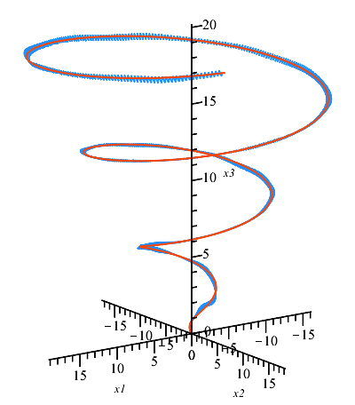
For numerical simulations, we choose ${y^{*}(t)=(0.2t\cos(0.2t),0.2t\sin(0.2t),0.2t)^{T}}$, $\omega_{1}(t)=0.25\cos(t)$ and put $\varepsilon=0.1,$ $\alpha=15$. Fig. 1 illustrates the behavior of system (8) with control (9) and the initial condition ${x^{0}=(0,0,0,\frac{\pi}{4},\frac{\pi}{4},\frac{\pi}{4})^{T}}$.

The presented case study demonstrates that our approach is applicable to the class of underactuated control-affine systems adhering to a specific Lie algebra rank condition, thereby encompassing essentially nonlinear dynamical behavior. On one hand, our method extends the paradigm of partial stabilization to encompass curve-following behaviors; on the other hand, it generalizes our earlier results by encompassing systems with non-zero drift and situations where the reference curve is defined in a lower dimensional subspace. The outcome of this work is oriented towards robotics, where there is a compelling need to stabilize only a portion of a system’s states, enhancing the control and maneuverability of robotic platforms across diverse and potentially unpredictable environments.

The proof of Theorem 1 combines and extends the techniques introduced in the papers [9, 11, 12]. Note that the results of those papers cannot be directly applied because of more general assumptions. In particular, we do not require the $z$-extendability of solutions.

Proof of Theorem 1. Given a $p>0,$ let us fix $\delta,$ $\delta^{{}^{\prime}}$ such that $0<\delta<\delta^{{}^{\prime}}$ and $B_{\delta^{{}^{\prime}}}(y^{*}(t))\subset D_{y}$ for all $t\geq 0.$ Denote $D^{{}^{\prime}}=B_{\delta^{{}^{\prime}}}(y^{*}(t))\times\mathbb{R}^{n_{2}}.$ From assumption A1.2), there exist positive constants $M_{g},$ $M_{h},$ $M_{g_{0}},$ $M_{h_{0}},$ $L_{g},$ $L_{h},$ $L_{g_{0}},$ $L_{h_{0}},$ $M_{g_{2}},$ $M_{g_{20}},$ $L_{g_{20}},$ $M_{g_{3}},$ $M_{g_{30}}$ such that for all $x,\tilde{x}\in D^{{}^{\prime}},$ $t,\tilde{t}\geq 0,$ and $k_{1},k_{2},k_{3}\in\{1,2,3,...,m\},$

		$\displaystyle\|y^{*}(t){-}y^{*}(\tilde{t})\|\leq L^{*}|t{-}\tilde{t}|,$
		$\displaystyle\|g_{0}(t,x)\|\leq M_{g_{0}},\,\|g_{k}(x)\|\leq M_{g},\,\left\|\frac{\partial g_{0}(t,x)}{\partial t}\right\|\leq L_{g_{20}},$
		$\displaystyle\|h_{0}(t,x)\|\leq M_{h_{0}},\,\|h_{k}(x)\|\leq M_{h},\,\|\mathcal{L}_{f_{k_{2}}}g_{k_{1}}(x)\|\leq M_{g_{2}},$
		$\displaystyle\|g_{0}(t,x){-}g_{0}(t,\tilde{x})\|\leq L_{g_{0}}\|x{-}\tilde{x}\|,$
		$\displaystyle\|h_{0}(t,x){-}h_{0}(t,\tilde{x})\|\leq L_{h_{0}}\|x{-}\tilde{x}\|,$
		$\displaystyle\|g_{k}(x){-}g_{k}(\tilde{x})\|\leq L_{g}\|x{-}\tilde{x}\|,\|h_{k}(x){-}h_{k}(\tilde{x})\|\leq L_{h}\|x{-}\tilde{x}\|,$
		$\displaystyle\max\{\|\mathcal{L}_{f_{0}}g_{0}(t,x)\|,\|\mathcal{L}_{f_{k}}g_{0}(t,x)\|,\,\|\mathcal{L}_{f_{0}}g_{k}(t,x)\|\}\leq M_{g_{20}},$
		$\displaystyle\|\mathcal{L}_{f_{k_{3}}}\mathcal{L}_{f_{k_{2}}}g_{k_{1}}(x)\|\leq M_{g_{3}},\,\|\mathcal{L}_{f_{0}}\mathcal{L}_{f_{k_{2}}}g_{k_{1}}(t,x)\|\leq M_{g_{30}}.$

Furthermore, assumption A1.1) implies the existence of a $\mu>0$ such that $\|\mathcal{F}^{-1}(x)\|\leq\mu$ for all $x\in D^{\prime},$ where $\mathcal{F}^{-1}(x)$ is the inverse matrix for $\mathcal{F}(x).$

Let $x^{0}=(y^{0^{T}},z^{0^{T}})^{T}\in B_{\delta}(\mathit{Y_{0}^{p}}),$ and denote

$${U^{\varepsilon}=\max\limits_{0\leq t\leq\varepsilon}\sum_{k=1}^{m}|u_{k}^{\varepsilon}(t,x^{0},y^{*}_{0})|.}$$

For the simplicity and without loss of generality, we put $t_{0}=0$. Using (7) and Hölder’s inequality, one can show that, for any $x^{0}\in B_{\delta}(\mathit{Y_{0}^{p}}),$

$$U^{\varepsilon}\leq c_{1}\|y^{0}-y_{0}^{*}\|+\frac{c_{2}}{\sqrt{\varepsilon}}\sqrt{\|y^{0}-y_{0}^{*}\|}\leq c_{u}\sqrt{\frac{\|y^{0}-y_{0}^{*}\|}{\varepsilon}},$$

(10)

where $c_{1}{=}\sqrt{|S_{1}|}\alpha\mu,$ ${c_{2}{=}2\sqrt{2\alpha\pi\mu}\left(\sum_{(j_{1}j_{2})\in S_{2}}(\kappa_{j_{1}j_{2}})^{\frac{2}{3}}\right)^{\frac{3}{4}}}$, and $c_{u}=c_{1}\sqrt{\varepsilon(p+\delta)}+c_{2}$.

The first step of the proof is to show that all solutions of system (4) with initial conditions in $B_{\delta}(\mathit{Y_{0}^{p}})$ are well defined in $D^{\prime}$ on the time interval $[0,\varepsilon]$ with some small enough ${\varepsilon>0.}$ Using the integral representation of the $y$-component of the solutions of system (4) with $x^{0}\in B_{\delta}(\mathit{Y_{0}^{p}})$, we get

	$\displaystyle\|y(t){-}y^{0}\|=$	$\displaystyle\Big{\|}\int\limits_{0}^{t}g_{0}(s,x(s))ds{+}\sum_{k=1}^{m}\int\limits_{0}^{t}g_{k}(x(s))u_{k}(s)ds\Big{\|}$
	$\displaystyle\leq$	$\displaystyle\int\limits_{0}^{t}\|g_{0}(s,x^{0})\|ds{+}\sum_{k=1}^{m}\|g_{k}(x^{0})\|\int\limits_{0}^{t}|u_{k}(s)|ds$
		$\displaystyle{+}\int\limits_{0}^{t}\|g_{0}(s,x(s)){-}g_{0}(s,x^{0})\|$
		$\displaystyle{+}\sum_{k=1}^{m}\|g_{k}(x(s)){-}g_{k}(x^{0})\||u_{k}(s)|ds$
	$\displaystyle\leq$	$\displaystyle(L_{0}{+}L_{g}U^{\varepsilon})\int\limits_{0}^{t}\Big{(}\|y(s){-}y^{0}\|{+}\|z(s){-}z^{0}\|\Big{)}ds$
		$\displaystyle{+}(M_{g_{0}}{+}M_{g}U^{\varepsilon})t.$

Similarly,

	$\displaystyle\|z(t){-}z^{0}\|$	$\displaystyle\leq(L_{h_{0}}{+}U^{\varepsilon}L_{h})\int\limits_{0}^{t}\left(\|y(s){-}y^{0}\|{+}\|z(s){-}z^{0}\|\right)ds$
		$\displaystyle{+}(M_{h_{0}}{+}U^{\varepsilon}M_{h})t.$

Applying Grönwall–Bellman inequality to the both estimates, we obtain:

	$\displaystyle\|y(t)-y^{0}\|\leq$	$\displaystyle e^{(L_{0}{+}L_{g}U^{\varepsilon})t}\Big{(}(M_{g_{0}}{+}U^{\varepsilon}M_{g})t$
		$\displaystyle{+}(L_{g_{0}}{+}U^{\varepsilon}L_{g})\int\limits_{0}^{t}\|z(s)-z^{0}\|ds\Big{)},$

	$\displaystyle\|z(t)-z^{0}\|\leq$	$\displaystyle e^{(L_{h_{0}}{+}U^{\varepsilon}L_{h})t}\Big{(}(M_{h_{0}}{+}U^{\varepsilon}M_{h})t$
		$\displaystyle{+}(L_{h_{0}}{+}U^{\varepsilon}L_{h})\int\limits_{0}^{t}\|y(s)-y^{0}\|ds\Big{)}.$

References

- [1] A. Aleksandrov, E. Aleksandrova, A. Zhabko, and C. Yangzhou. Partial stability analysis of some classes of nonlinear systems. Acta Mathematica Scientia, 37(2):329–341, 2017.
- [2] J. Barraquand and J.-C. Latombe. On nonholonomic mobile robots and optimal maneuvering. In Proc. IEEE International Symposium on Intelligent Control, pages 340–347, 1989.
- [3] T. Binazadeh and M.J. Yazdanpanah. Application of passivity based control for partial stabilization. Nonlinear Dynamics and Systems Theory, 11(4):373–382, 2011.
- [4] V. Chellaboina and W. M. Haddad. A unification between partial stability and stability theory for time-varying systems. IEEE Control Systems Magazine, 22(6):66–75, 2002.
- [5] H. Chen, B. Li, B. Zhang, and L. Zhang. Global finite-time partial stabilization for a class of nonholonomic mobile robots subject to input saturation. International Journal of Advanced Robotic Systems, 12(11):159, 2015.
- [6] F. H. Clarke, Y. S. Ledyaev, E. D. Sontag, and A. I. Subbotin. Asymptotic controllability implies feedback stabilization. IEEE Tran on Automatic Control, 42(10):1394–1407, 1997.
- [7] M. Golestani, I. Mohammadzaman, and M. J. Yazdanpanah. Robust finite-time stabilization of uncertain nonlinear systems based on partial stability. Nonlinear Dynamics, 85(1):87–96, 2016.
- [8] V. Grushkovskaya and A. Zuyev. Obstacle avoidance problem for second degree nonholonomic systems. In Proc. 57th IEEE Conf. on Decision and Control, pages 1500–1505, 2018.
- [9] V. Grushkovskaya and A. Zuyev. Partial stability concept in extremum seeking problems. IFAC-PapersOnLine, 52(16):682–687, 2019.
- [10] V. Grushkovskaya and A. Zuyev. Stabilization of non-admissible curves for a class of nonholonomic systems. In 2019 18th European Control Conference (ECC), pages 656–661. IEEE, 2019.
- [11] V. Grushkovskaya and A. Zuyev. Partial stabilization of nonholonomic systems with application to multi-agent coordination. In Proc. of the 2020 European Control Conference (ECC), pages 1665–1670, 2020.
- [12] V. Grushkovskaya and A. Zuyev. Motion planning and stabilization of nonholonomic systems using gradient flow approximations. Nonlinear Dynamics, 2023.
- [13] W. M. Haddad and A. L’Afflitto. Finite-time partial stability and stabilization, and optimal feedback control. Journal of the Franklin Institute, 352(6):2329–2357, 2015.
- [14] Z. Hai-ping and M. Feng-xiang. On the stability of nonholonomic mechanical systems with respect to partial variables. Applied Mathematics and Mechanics, 16(3):237–245, 1995.
- [15] E. J. Hancock and D. J. Hill. Restricted partial stability and synchronization. IEEE Transactions on Circuits and Systems I: Regular Papers, 61(11):3235–3244, 2014.
- [16] C. Jammazi. Continuous and discontinuous homogeneous feedbacks finite-time partially stabilizing controllable multichained systems. SIAM Journal on Control and Optimization, 52(1):520–544, 2014.
- [17] J.-G. Jian and X.-X. Liao. Partial exponential stability of nonlinear time-varying large-scale systems. Nonlinear Analysis: Theory, Methods & Applications, 59(5):789–800, 2004.
- [18] O. Kolesnichenko and A. S. Shiriaev. Partial stabilization of underactuated Euler–Lagrange systems via a class of feedback transformations. Systems & Control Letters, 45(2):121–132, 2002.
- [19] A. L’Afflitto, W. M. Haddad, and E. Bakolas. Partial-state stabilization and optimal feedback control. International Journal of Robust and Nonlinear Control, 26(5):1026–1050, 2016.
- [20] F Lamnabhi-Lagarrigue. Volterra and Fliess series expansions for nonlinear systems. In W. S. Levine, editor, The Control Handbook, pages 879–888. CRC Press, 1995.
- [21] J. A. Langa, J. C. Robinson, and A. Suárez. Stability, instability, and bifurcation phenomena in non-autonomous differential equations. Nonlinearity, 15(3):887, 2002.
- [22] A.N. Michel, A.P. Molchanov, and Y. Sun. Partial stability of discontinuous dynamical systems. In Proceedings of the 2002 American Control Conference (IEEE Cat. No. CH37301), volume 1, pages 74–79. IEEE, 2002.
- [23] Arkadiusz Mielczarek and Ignacy Duleba. Development of task-space nonholonomic motion planning algorithm based on Lie-algebraic method. Applied Sciences, 11(21):10245, 2021.
- [24] I. V. Miroshnik. Partial stabilization and geometric problems of nonlinear control. IFAC Proceedings Volumes, 35(1):151–156, 2002.
- [25] I. V. Miroshnik. Attractors and partial stability of nonlinear dynamical systems. Automatica, 40(3):473–480, 2004.
- [26] M. Panda, B. Das, B. Subudhi, and B. B. Pati. A comprehensive review of path planning algorithms for autonomous underwater vehicles. International Journal of Automation and Computing, 17(3):321–352, 2020.
- [27] Y. Qin, Y. Kawano, B. D.O. Anderson, and M. Cao. Partial exponential stability analysis of slow-fast systems via periodic averaging. IEEE Transactions on Automatic Control, 2021.
- [28] T. Rajpurohit and W. M. Haddad. Partial-state stabilization and optimal feedback control for stochastic dynamical systems. Journal of Dynamic Systems, Measurement, and Control, 139(9):091001, 2017.
- [29] A. Rizaldi, F. Immler, B. Schürmann, and M. Althoff. A formally verified motion planner for autonomous vehicles. In International Symposium on Automated Technology for Verification and Analysis, pages 75–90. Springer, 2018.
- [30] P. Rousseas, C. P. Bechlioulis, and K. J. Kyriakopoulos. Trajectory planning in unknown 2d workspaces: A smooth, reactive, harmonics-based approach. IEEE Robotics and Automation Letters, 7(2):1992–1999, 2022.
- [31] V. V. Rumyantsev and A. S. Oziraner. Stability and Stabilization of Motion with Respect to Part of the Variables. Nauka, 1987. (in Russian).
- [32] A.S. Shiriaev and O. Kolesnichenko. On passivity based control for partial stabilization of underactuated systems. In Proc. 39th IEEE Conf. on Decision and Control, volume 3, pages 2174–2179, 2000.
- [33] X. Sun, G. Wang, and Y. Fan. Adaptive trajectory tracking control of vector propulsion unmanned surface vehicle with disturbances and input saturation. Nonlinear Dynamics, 106(3):2277–2291, 2021.
- [34] Y. Sun and A. N. Michel. Partial stability of general dynamical systems under arbitrary initial z-perturbations. In Proc. 41st IEEE Conf. on Decision and Control, volume 3, pages 2663–2668, 2002.
- [35] V. I. Vorotnikov. Partial stability and control. Springer Science & Business Media, 2012.
- [36] V. I. Vorotnikov and Y. G. Martyshenko. On the partial stability in probability of nonlinear stochastic systems. Automation and Remote Control, 80(5):856–866, 2019.
- [37] B. Wang, H. Ashrafiuon, and S. Nersesov. Leader–follower formation stabilization and tracking control for heterogeneous planar underactuated vehicle networks. Systems & Control Letters, 156:105008, 2021.
- [38] A. Zuiev. On Brockett’s condition for smooth stabilization with respect to a part of the variables. In 1999 European Control Conference (ECC), pages 1729–1732. IEEE, 1999.
- [39] A. Zuyev. Stabilization of non-autonomous systems with respect to a part of variables by means of controlled lyapunov functions. Journal of Automation and Information Sciences, 32(10), 2000.
- [40] A. Zuyev. Application of control lyapunov functions technique for partial stabilization. In Proceedings of the 2001 IEEE International Conference on Control Applications (CCA’01), pages 509–513. IEEE, 2001.
- [41] A Zuyev. Partial asymptotic stability and stabilization of nonlinear abstract differential equations. In Proc. 42nd IEEE Conf on Decision and Control, volume 2, pages 1321–1326, 2003.
- [42] A. Zuyev. Partial asymptotic stability of abstract differential equations. Ukrainian Mathematical Journal, 58(5):709–717, 2006.
- [43] A. Zuyev. Exponential stabilization of nonholonomic systems by means of oscillating controls. SIAM Journal on Control and Optimization, 54(3):1678–1696, 2016.
- [44] A. Zuyev and I. Vasylieva. Partial stabilization of stochastic systems with application to rotating rigid bodies. IFAC-PapersOnLine, 52(16):162–167, 2019.