Partial Identification of Dose Responses with Hidden Confounders

Myrl G. Marmarelis USC Information Sciences Institute
4676 Admiralty Way
Marina del Rey, CA 90292 Elizabeth Haddad USC Stevens Neuroimaging and Informatics Institute
4676 Admiralty Way
Marina del Rey, CA 90292 Andrew Jesson University of Oxford, OATML
14 Parks Road
Oxford, UK OX1 3AQ
Neda Jahanshad USC Stevens Neuroimaging and Informatics Institute
4676 Admiralty Way
Marina del Rey, CA 90292 Aram Galstyan USC Information Sciences Institute
4676 Admiralty Way
Marina del Rey, CA 90292 Greg Ver Steeg USC Information Sciences Institute
4676 Admiralty Way
Marina del Rey, CA 90292

Abstract

Inferring causal effects of continuous-valued treatments from observational data is a crucial task promising to better inform policy- and decision-makers. A critical assumption needed to identify these effects is that all confounding variables—causal parents of both the treatment and the outcome—are included as covariates. Unfortunately, given observational data alone, we cannot know with certainty that this criterion is satisfied. Sensitivity analyses provide principled ways to give bounds on causal estimates when confounding variables are hidden. While much attention is focused on sensitivity analyses for discrete-valued treatments, much less is paid to continuous-valued treatments. We present novel methodology to bound both average and conditional average continuous-valued treatment-effect estimates when they cannot be point identified due to hidden confounding. A semi-synthetic benchmark on multiple datasets shows our method giving tighter coverage of the true dose-response curve than a recently proposed continuous sensitivity model and baselines. Finally, we apply our method to a real-world observational case study to demonstrate the value of identifying dose-dependent causal effects.

1 Introduction

Causal inference on observational studies [Hill, 2011, Athey et al., 2019] attempts to predict conclusions of alternate versions of those studies, as if they were actually properly randomized experiments. The causal aspect is unique among inference tasks in that the goal is not prediction per se, as causal inference deals with counterfactuals, the problem of predicting unobservables: for example, what would have been a particular patient’s health outcome had she taken some medication, versus not, while keeping all else equal (ceteris paribus)? There is quite often no way to validate the results without bringing in additional domain knowledge. A set of putative treatments $\mathcal{T}$ , often binary with a treated/untreated dichotomy, induces potential outcomes $Y_{t\in\mathcal{T}}$ . These can depend on covariates $X$ as with heterogeneous treatment effects $\operatorname{\mathbb{E}}[Y_{1}-Y_{0}\mid X]$ in the binary case. Only one outcome is ever observed: that at the assigned treatment $T$ . Potential biases arise from the incomplete observation. This problem is exacerbated with more than two treatment values, especially when there are infinite possibilities, like in a continuum, e.g. $\mathcal{T}=[0,1]$ . Unfortunately, many consequential decisions in life involve this kind of treatment: What dose of drug should I take? How much of should I eat/drink? How much exercise do I really need?

In an observational study, the direct causal link between assigned treatment $T$ and observed outcome $Y$ (also denoted as $Y_{T}$ ) can be influenced by indirect links modulated by confounding variables. For instance, wealth is often a confounder in an individual’s health outcome from diet, medication, or exercise. Wealth affects access to each of these “treatments,” and it also affects health through numerous other paths. Including the confounders as covariates in $X$ allows estimators to condition on them and disentangle the influences [Yao et al., 2021].

It can be challenging to collect sufficient data, in terms of quality and quantity, on confounders in order to adjust a causal estimation to them. Case in point, noisy observations of e.g. lifestyle confounders lead researchers to vacillate on the health implications of coffee [Atroszko, 2019], alcohol [Ystrom et al., 2022], and cheese [Godos et al., 2020].

For consequential real-world causal inference, it is only prudent to allow margins for some amount of hidden confounding. A major impediment to such analysis is that it is impossible to know how a hidden confounder would bias the causal effect. The role of any causal sensitivity model [Cornfield et al., 1959, Rosenbaum and Rubin, 1983] is to make reasonable structural assumptions [Manski, 2003] about different levels of hidden confounding. Most sensitivity analyses to hidden confounding require the treatment categories to be binary or at least discrete. This weakens empirical studies that are better specified by dose-response curves [Calabrese and Baldwin, 2001, Bonvini and Kennedy, 2022] from a continuous treatment variable. Estimated dose-response functions are indeed vulnerable in the presence of hidden confounders. Figure 1 highlights the danger of skewed observational studies that lead to biased estimates of personal toxic thresholds of treatment dosages.

Refer to caption — Figure 1: Dose-respone curves in medicine [e.g. Taleb, 2018] can be viewed as expected potential outcomes from continuous treatments. In this simulation (with details in §D,) there is one unobserved confounder. The empirical estimate of the population-level dose responses massively overshoots the maximum effective dosage, and would suggest treatments that were actually toxic to the population. This phenomenon persists even when the vulnerable hidden subgroup occurs more often in the population.

1.1 Related works

There is growing interest in causal methodology for continuous treatments (or exposures, interventions), especially in the fields of econometrics [e.g. Huang et al., 2021, Tübbicke, 2022], health sciences [Vegetabile et al., 2021], and machine learning [Chernozhukov et al., 2021, Ghassami et al., 2021, Colangelo and Lee, 2021, Kallus and Santacatterina, 2019]. So far, most scrutiny on partial identification of potential outcomes has focused on the case of discrete treatments [e.g. Rosenbaum and Rubin, 1983, Louizos et al., 2017, Lim et al., 2021]. A number of creative approaches recently made strides in the discrete setting. Most rely on a sensitivity model for assessing the susceptibility of causal estimands to hidden-confounding bias. A sensitivity model allows hidden confounders but restricts their possible influence on the data, with an adjustable parameter that controls the overall tightness of that restriction.

The common discrete-treatment sensitivity models are incompatible with continuous treatments, which are needed for estimating dose-response curves. Still, some recent attempts have been made to handle hidden confounding under more general treatment domains [Chernozhukov et al., 2021]. Padh et al. [2022], Hu et al. [2021] optimize generative models to reflect bounds on the treatment effect due to ignorance, inducing an implicit sensitivity model through functional constraints. Instrumental variables are also helpful when they are available [Kilbertus et al., 2020]. The CMSM [Jesson et al., 2022] was developed in parallel to this work, and now serves as a baseline.

For binary treatments, the Marginal Sensitivity Model (MSM) due to Tan [2006] has found widespread usage [Zhao et al., 2019, Veitch and Zaveri, 2020, Yin et al., 2021, Kallus et al., 2019, Jesson et al., 2021]. Variations thereof include Rosenbaum’s earlier sensitivity model [2002] that enjoys ties to regression coefficients [Yadlowsky et al., 2020]. Alternatives to sensitivity models leverage generative modeling [Meresht et al., 2022] and robust optimization [Guo et al., 2022]. Other perspectives require additional structure to the data-generating (observed outcome, treatment, covariates) process. Proximal causal learning [Tchetgen et al., 2020, Mastouri et al., 2021] requires observation of proxy variables. Chen et al. [2022] rely on a large number of background variables to help filter out hidden confounding from apparent causal influences.

1.2 Contributions

We propose a novel sensitivity model for continuous treatments in §2. Next, we derive general formulas (§2.1) and solve closed forms for three versions (§2.3) of partially identified dose responses—for Beta, Gamma, and Gaussian treatment variables. We devise an efficient sampling algorithm (§3), and validate our results empirically using a semi-synthetic benchmark (§4) and realistic case study (§5).

1.3 Problem Statement

Our goal is the partial identification of causal dose responses under a bounded level of possible hidden confounding. We consider any setup that grants access to two predictors [Chernozhukov et al., 2017] that can be learned empirically and are assumed to output correct conditional distributions. These are (1) a predictor of outcomes conditioned on covariates and the assigned treatment, and (2) a predictor of the propensity of treatment assignments, taking the form of a probability density, conditioned on the covariates. The latter measures (non-)uniformity in treatment assignment for different parts of the population. The observed data come from a joint distribution of outcome, continuous treatment, and covariates that include any observed confounders.

Potential outcomes.

Causal inference is often cast in the nomenclature of potential outcomes, due to Rubin [1974]. Our first assumption, common to Rubin’s framework, is that observation tuples of outcome, assigned treatment, and covariates, $\{(y^{(i)},t^{(i)},x^{(i)})\}_{i=1}^{n},$ are i.i.d draws from a single joint distribution. This subsumes the Stable Unit Treatment Value Assumption (SUTVA), where units/individuals cannot depend on one another, since they are i.i.d. The second assumption is overlap/positivity, that all treatments have a chance of assignment for every individual in the data: ${p_{T\mid X}(t\mid x)>0}$ for every ${(t,x)\in\mathcal{T}\times\mathcal{X}}$ .

The third and most challenging fundamental assumption is that of ignorability/sufficiency: ${\{(Y_{t})_{t\in\mathcal{T}}\mathbin{\perp\!\!\!\perp}T\}\mid X}.$ Clearly the outcome should depend on the assigned treatment, but potential outcomes ought not to be affected by the assignment, after blocking out paths through covariates.

Our study focuses on dealing with limited violations to ignorability. The situation is expressed formally as $\{(Y_{t})_{t\in\mathcal{T}}\mathbin{\not\!\perp\!\!\!\perp}T\}\mid X$ , but more specifically, we shall introduce a sensitivity model that governs the shape and extent of that violation.

Let $p(y_{t}|x)$ denote the probability density function of potential outcome $Y_{t}=y_{t}$ from a treatment $t\in\mathcal{T}$ , given covariates $X=x$ . This is what we seek to infer, while observing realized outcomes that allow us to learn the density $p(y_{t}|\,x,\,T=t)$ . If the ignorability condition held, then $p(y_{t}|\,x,\,T=t)=p(y_{t}|x)$ due to the conditional independence. However, without ignorability, one has to marginalize over treatment assignment, requiring $p(y_{t}|\,x,\,T\neq t)$ because

p(y_{t}|x)=\int_{\mathcal{T}}p(y_{t}|\,\tau,x)p(\tau|x)\operatorname{\mathrm{d}\!}\tau,

(1)

where $p(y_{t}|\tau,x)$ is the distribution of potential outcomes conditioned on actual treatment $T=\tau\in\mathcal{T}$ that may differ from the potential outcome’s index $t$ . The density $p(\tau|x)$ is termed the nominal propensity, defining the distribution of treatment assignments for different covariate values.

On notation.

Throughout this study, $y_{t}$ will indicate the value of the potential outcome at treatment $t$ , and to disambiguate with assigned treatment $\tau$ will be used for events where $T=\tau$ . For instance, we may care about the counterfactual of a smoker’s $(\tau=1)$ health outcome had they not smoked $(y_{t=0}),$ where $T=0$ signifies no smoking and $T=1$ is “full” smoking. We will use the shorthand $p(\cdots)$ with lowercase variables whenever working with probability densities of the corresponding variables in uppercase:

\displaystyle p(y_{t}|\tau,x)\

\displaystyle\textrm{ means }\ \frac{\partial}{\partial u}\mathbb{P}[\,Y_{t}\leq u\mid T=\tau,\ X=x\,]\Big{\rvert}_{u=y_{t}.}

Quantities of interest.

We attempt to impart intuition on the conditional probability densities that may be confusing.

•

$p(y_{t}|\,x)$ [conditional potential outcome]. A person’s outcome from a treatment, disentangled from the selection bias of treatment assignment in the population. We seek to characterize this in order to (partially) identify the Conditional Average Potential Outcome (CAPO) and the Average Potential Outcome (APO):

$\text{CAPO}(t,x)=\operatorname{\mathbb{E}}[Y_{t}\mid X=x];\quad\text{APO}(t)=\operatorname{\mathbb{E}}[Y_{t}].$
•

$p(y_{t}|\,\tau,x)$ [counterfactual]. What is the potential outcome of a person in the population characterized by $x$ and assigned treatment $\tau$ ? The answer changes with $\tau$ only when $x$ is inadequate to block all backdoor paths through confounders. We can estimate this for $t=\tau$ .
•

$p(\tau|\,y_{t},x)$ [complete propensity] is related to the above by Bayes’ rule. We distinguish it from the nominal propensity $p(\tau|x)$ because the unobservable $y_{t}$ possibly confers more information about the individual, again if $x$ is inadequate. The complete propensity cannot be estimated, even for $t=\tau$ ; hence, this is the target of our sensitivity model.

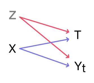
A backdoor path between potential outcomes and treatment can manifest in several ways. Figure 2 shows the barebones setting for hidden confounding to take place. Simply noisy observations of the confounders could leak a backdoor path. It is important to understand the ontology [Sarvet and Stensrud, 2022] of the problem in order to ascribe hidden confounding to the stochasticity inherent to a potential outcome.

Sensitivity.

Explored by Tan [2006] followed by Kallus et al. [2019], Jesson et al. [2021], among many others, the Marginal Sensitivity Model (MSM) serves to bound the extent of (putative) hidden confounding in the regime of binary treatments $T^{\prime}\in\{0,1\}$ . The MSM limits the discrepancy between the odds of treatment under the nominal propensity and the odds of treatment under the complete propensity.

Definition 1 (The Marginal Sensitivity Model).

For binary treatment $t^{\prime}\in\{0,1\}$ and violation factor $\Gamma\geq 1$ , the following ratio is bounded:

\Gamma^{-1}\leq\left[\frac{p(t^{\prime}|x)}{1-p(t^{\prime}|x)}\right]^{\,-1}\left[\frac{p(t^{\prime}|\,y_{t^{\prime}},x)}{1-p(t^{\prime}|\,y_{t^{\prime}},x)}\right]\leq\Gamma.

The confines of a binary treatment afford a number of conveniences. For instance, one probability value is sufficient to describe the whole propensity landscape on a set of conditions, $p(1-t^{\prime}|\cdots)=1-p(t^{\prime}|\cdots)$ . As we transfer to the separate context of treatment continua, we must contend with infinite treatments and infinite potential outcomes.

2 Continuous Sensitivity Model

The counterfactuals required for Equation 1 are almost entirely unobservable. We look to the Radon-Nikodym derivative $\omega_{\delta}$ of a counterfactual with respect to another [Tan, 2006], quantifying their divergence between nearby treatment assignments: (assuming mutual continuity)

	$\displaystyle\omega_{\delta}(y_{t}\|\,\tau,x)\coloneqq$	$\displaystyle\ \frac{p(y_{t}\|\,\tau+\delta,x)}{p(y_{t}\|\,\tau,x)}\ =\ \ \stackrel{{\scriptstyle\text{(Bayes' rule)}}}{{\frac{p(\tau+\delta\|\,y_{t},x)p(\tau\|x)}{p(\tau\|\,y_{t},x)p(\tau+\delta\|x)}}}$
		$\displaystyle=\left[\frac{p(\tau+\delta\|x)}{p(\tau\|x)}\right]^{\,-1}\left[\frac{p(\tau+\delta\|\,y_{t},x)}{p(\tau\|\,y_{t},x)}\right].$

As with the MSM, we encounter a ratio of odds, here contrasting $\tau$ versus $\tau+\delta$ in the assigned-treatment continuum. Assuming the densities are at least once differentiable,

\lim_{\delta\to 0}\delta^{-1}\log\omega_{\delta}(y_{t}|\,\tau,x)=\partial_{\tau}[\log p(\tau|\,y_{t},x)-\log p(\tau|x)].

By constraining $\omega_{\delta}$ to be close to unit, via bounds above and below, we tie the logarithmic derivatives of the nominal- and complete-propensity densities.

Definition 2 (The Infinitesimal Marginal Sensitivity Model).

For treatments $t\in\mathcal{T}\subseteq\mathbb{R}$ , where $\mathcal{T}$ is connected, and violation-of-ignorability factor $\Gamma\geq 1$ , the $\delta$ MSM requires

\absolutevalue{\frac{\partial}{\partial\tau}\log\frac{p(\tau|\,y_{t},x)}{p(\tau|x)}}\leq\log\Gamma

everywhere, for all $\tau$ , $t$ , and $x$ combinations. This differs from the CMSM due to Jesson et al. [2022] that considers only $t=\tau,$ and which bounds the density ratios directly.

2.1 The Complete Framework

Assumption 1 (Bounded Hidden Confounding).

Invoking Definition 2, the violation of ignorability is constrained by a $\delta$ MSM with some $\Gamma\geq 1$ .

Assumption 2 (Anchor Point).

A special treatment value designated as zero is not informed by potential outcomes: $p(\tau=0\mid y_{t},x)=p(\tau=0\mid x)$ for all $x$ , $t$ , and $y_{t}$ .

At this point we state the core sensitivity assumptions. In addition to the $\delta$ MSM, we require an anchor point at $T=0$ , which may be considered a lack of treatment. Strictly, we assume that hidden confounding does not affect the propensity density precisely at the anchor point. A broader interpretation is that the strength of causal effect, hence vulnerability to hidden confounders, roughly increases with $\absolutevalue{T}$ . Assumption 2 is necessary to make closed-form solutions feasible. We discuss ramifications and a relaxation in §2.3.

The unobservability of almost all counterfactuals is unique to the case of continuous treatments, since the discrete analogy would be a discrete sum with an observable term. Figure 3 explains our approach to solving Equation 1.

2.2 A Partial Approximation

We expand $p(y_{t}|\tau,x)$ around $\tau=t,$ where $p(y_{t}|t,x)=p(y|t,x)$ is learnable from data. Suppose that $p(y_{t}|\tau,x)$ is twice differentiable in $\tau$ . Construct a Taylor expansion

p(y_{t}|\tau,x)=p(y_{t}|t,x)+(\tau-t)\partial_{\tau}p(y_{t}|\tau,x)|_{\tau=t}\\ +\frac{(\tau-t)^{2}}{2}\partial^{2}_{\tau}p(y_{t}|\tau,x)|_{\tau=t}+\mathcal{O}(\tau-t)^{3}.

(2)

Denote with $\tilde{p}(y_{t}|\tau,x)$ an approximation of second order as laid out above. One could have stopped at lower orders but the difference in complexity is not that large. The intractable derivatives like $\partial_{\tau}p(y_{t}|\tau,x)|_{\tau=t}$ will be bounded using the $\delta$ MSM machinery. Let us quantify the reliability of this approximation by a trust-weighing scheme $0\leq w_{t}(\tau)\leq 1,$ where typically $w_{t}(t)=1.$ This corresponds to the yellow part in Figure 3. We argue that $w_{t}(\tau)$ should be narrower with lower-entropy (narrower) propensities (§B). The possible forms of $w_{t}(\tau)$ are elaborated in §2.3.

Splitting Equation 1 along the trusted regime marked by $w_{t}(\tau)$ , and then applying the approximation of Equation 2,

$\displaystyle p(y_{t}\|x)=$	$\displaystyle\int_{\mathcal{T}}\underbrace{w_{t}(\tau)p(y_{t}\|\tau,x)p(\tau\|x)\operatorname{\mathrm{d}\!}\tau}_{\text{``observable'' (Fig.\leavevmode\nobreak\ \ref{fig:math-outline})}}$	(3)
	$\displaystyle+\int_{\mathcal{T}}\underbrace{[1-w_{t}(\tau)]p(y_{t}\|\tau,x)p(\tau\|x)\operatorname{\mathrm{d}\!}\tau}_{\text{``unobservable'' (Fig.\leavevmode\nobreak\ \ref{fig:math-outline})}}$
$\displaystyle{\color[rgb]{0.9,0,0}\definecolor[named]{pgfstrokecolor}{rgb}{0.9,0,0}\approx}$	$\displaystyle\int_{\mathcal{T}}\,\underbrace{w_{t}(\tau){\color[rgb]{0.9,0,0}\definecolor[named]{pgfstrokecolor}{rgb}{0.9,0,0}\tilde{p}}(y_{t}\|\tau,x)p(\tau\|x)\operatorname{\mathrm{d}\!}\tau}_{(A)\text{ the approximated quantity}}$
	$\displaystyle+\int_{\mathcal{T}}\,\underbrace{[1-w_{t}(\tau)]p(\tau\|y_{t},x)p(y_{t}\|x)\operatorname{\mathrm{d}\!}\tau}_{(B)\text{ by Bayes' rule}}.$

The intuition behind separating the integral into two parts is the following. By choosing the weights $w_{t}(\tau)$ so that they are close to one in the range where approximation Equation 2 is valid (yellow region in Figure 3) and zero outside of this range, we can evaluate the first integral through the approximated counterfactuals. The second integral, which is effectively over the red region in Figure 3 and cannot be evaluated due to unobserved counterfactuals, will be bounded using the $\delta$ MSM. Simplifying the second integral first,

\int_{\mathcal{T}}[1-w_{t}(\tau)]p(\tau|\,y_{t},x)p(y_{t}|x)\operatorname{\mathrm{d}\!}\tau\\ =p(y_{t}|x)\left[1-\int_{\mathcal{T}}w_{t}(\tau)p(\tau|\,y_{t},x)\operatorname{\mathrm{d}\!}\tau\right].

By algebraic manipulation, we witness already that $p(y_{t}|x)$ shall take the form of

p(y_{t}|x)\approx\frac{\int_{\mathcal{T}}w_{t}(\tau)\tilde{p}(y_{t}|\,\tau,x)p(\tau|x)\operatorname{\mathrm{d}\!}\tau}{\int_{\mathcal{T}}w_{t}(\tau)p(\tau|\,y_{t},x)\operatorname{\mathrm{d}\!}\tau}.

(4)

Reflecting on Assumptions 1 & 2, the divergence between $p(\tau|\,y_{t},x)$ and $p(\tau|x)$ is bounded, allowing characterization of the denominator in terms of the learnable $p(\tau|x)$ . Similarly the derivatives in Equation 2 can be bounded. These results would be sufficient to partially identify the numerator. Without loss of generality, consider the unknown quantity $\gamma$ that can be a function of $\tau$ , $y_{t}$ , and $x$ , such that

\partial_{\tau}\log p(\tau|y_{t},x)=\partial_{\tau}\log p(\tau|x)+\gamma(\tau|y_{t},x),\\ \text{where }\absolutevalue{\gamma(\tau|y_{t},x)}\leq\log\Gamma\text{ using the $\delta$MSM.}

(5)

We may attempt to integrate both sides;

$\displaystyle\int_{0}^{\,s}\partial_{\tau}\log p(\tau\|\,y_{t},x)\operatorname{\mathrm{d}\!}\tau=$	$\displaystyle\int_{0}^{\,s}\partial_{\tau}\log p(\tau\|x)\operatorname{\mathrm{d}\!}\tau$
	$\displaystyle\ \ +\underbrace{\int_{0}^{\,s}\gamma(\tau\|y_{t},x)\operatorname{\mathrm{d}\!}\tau}_{\coloneqq\lambda(s\|y_{t},x)}.$
$\displaystyle\therefore\log p(\tau=s\|\,y_{t},x)-\log$	$\displaystyle\,p(\tau=0\|\,y_{t},x)$
$\displaystyle=\log p(\tau=s\|\,x)-$	$\displaystyle\log p(\tau=0\|\,x)+\lambda(s\|y_{t},x),$
$\displaystyle\therefore\log p(\tau\|\,y_{t},x)=\log p(\tau\|$	$\displaystyle x)+\lambda(\tau\|y_{t},x).$
(by Assumption 2)
$\displaystyle\therefore\quad p(\tau\|\,y_{t},x)=p(\tau\|x)\Lambda$	$\displaystyle(\tau\|y_{t},x),\ \ \Lambda\coloneqq\exp{\lambda}.$	(6)

One finds that $\absolutevalue{\lambda(\tau|y_{t},x)}\leq\absolutevalue{\tau}\log\Gamma$ because $\lambda$ integrates $\gamma$ , bounded by $\pm\log\Gamma,$ over a support with length $\tau$ . Subsequently, $\Lambda$ is bounded by $\Gamma^{\pm\absolutevalue{\tau}}.$ These are the requisite tools for bounding $p(y_{t}|x)$ —or an approximation thereof, erring on ignorance via the trusted regime marked by $w_{t}(\tau).$ The derivation is completed in §A by framing the unknown quantities in terms of $\gamma$ and $\Lambda$ , culminating in Equation 7.

Predicting potential outcomes.

The recovery of a fully normalized probability density $\tilde{p}(y_{t}|x)$ via Equation 4 is laid out below. It may be approximated with Monte Carlo or solved in closed form with specific formulations for the weights and propensity. Concretely, it takes on the form $\tilde{p}(y_{t}|x)=d(t|y_{t},x)^{-1}p(y_{t}|t,x),$ where

d(t|y_{t},x)\coloneqq\operatorname{\mathbb{E}}_{\tau}[\Lambda(\tau|y_{t},x)]-[\gamma\Lambda](t|y_{t},x)\,\operatorname{\mathbb{E}}_{\tau}[\tau-t]\\ -\frac{1}{2}[(\dot{\gamma}+\gamma^{2})\Lambda](t|y_{t},x)\,\operatorname{\mathbb{E}}_{\tau}[(\tau-t)^{2}],

(7)

and said expectations, $\operatorname{\mathbb{E}}_{\tau}[\cdot],$ are with respect to the implicit distribution $q(\tau|t,x)\propto w_{t}(\tau)p(\tau|x).$ The notation $\dot{\gamma}$ denotes a derivative in the first argument of $\gamma(t|y_{t},x).$

Assumption 3 (Second-order Simplification).

The quantity $\dot{\gamma}(\tau|y_{t},x)$ cannot be characterized as-is. Granting that $\gamma^{2}$ dominates over the former, and consequently

\absolutevalue{(\dot{\gamma}+\gamma^{2})\Lambda}\leq\absolutevalue{\gamma^{2}\Lambda}+\varepsilon\quad\textrm{for small }\varepsilon\geq 0.

Parametrization	Support $(\mathcal{T})$	Params.	Precision ( $r$ )	Bounds for $\operatorname{\mathbb{E}}_{\tau}[\Lambda(\tau\|y_{t},x)]$
Beta	$[0,1]$	$\alpha,\beta$	$\alpha+\beta-2$	${}_{1}F_{1}(\bm{\alpha}+1;\ \bm{\alpha}+\bm{\beta}+2;\ \pm\log\Gamma)$
				where $\bm{\alpha}\coloneqq\bar{\alpha}+\alpha-2,\ \bm{\beta}\coloneqq\bar{\beta}+\beta-2$
Balanced Beta	$[0,1]$	$\alpha,\beta$	$\alpha+\beta-2$	$t\cdot\langle\textrm{the {Beta} above}\rangle+(1-t)\cdot\langle\textrm{{Beta}, mirrored}\rangle$
Gamma	$[0,+\infty)$	$\alpha,\beta$	$\alpha/\beta^{2}$	$[1-(\pm\log\Gamma)/\bm{\beta}]^{-\bm{\alpha}}$
				where $\bm{\alpha}\coloneqq\bar{\alpha}+\alpha-1,\ \bm{\beta}\coloneqq\bar{\beta}+\beta$
Gaussian	$(-\infty,+\infty)$	$\mu,\sigma$	$1/\sigma$	$\exp{\bm{\sigma}^{2}(\log\Gamma)^{2}/2}\left(\begin{aligned} \Gamma^{\pm\bm{\mu}}[1+\erf&(\textstyle\frac{\bm{\mu}\pm\bm{\sigma}^{2}\log\Gamma}{\sqrt{2}\bm{\sigma}})]\\ +&\\ \Gamma^{\mp\bm{\mu}}[1-\erf&(\textstyle\frac{\bm{\mu}\mp\bm{\sigma}^{2}\log\Gamma}{\sqrt{2}\bm{\sigma}})]\end{aligned}\right)$
				where $\bm{\mu}\coloneqq\frac{\mu\bar{\sigma}^{2}+\bar{\mu}\sigma^{2}}{\bar{\sigma}^{2}+\sigma^{2}},\ \bm{\sigma}^{2}\coloneqq\frac{\bar{\sigma}^{2}\sigma^{2}}{\bar{\sigma}^{2}+\sigma^{2}}$

Table 1: Candidates for propensity and trust-weighing combinations. Each row specifies the distribution—beta, beta, gamma, and Gaussian respectively—of the propensity model

p(\tau|x).

The last column lists solutions for the first term of Equation 7 / 8. This is a convolution of the propensity and weighing scheme, which have similar forms (see Bromiley [2003] for the Gaussian case.) We distinguish the replicated parameters between propensity and weight by placing a bar over the propensity parameters. So if the propensity is

x\mapsto(\bar{\alpha},\bar{\beta})

, then the weighing scheme has

t\mapsto(\alpha,\beta).

The bold parameters are of the compound density, with respect to which the first and second moments are computed in Equation 7 / 8.

To make use of the formula in Equation 7, one first obtains the set of admissible $d(t|y_{t},x)\in\big{[}\,\underline{d}(t|y_{t},x),\overline{d}(t|y_{t},x)\,\big{]}$ that violate ignorability up to a factor $\Gamma$ according to the $\delta$ MSM. With the negative side of the $\pm$ corresponding to $\underline{d}$ and the positive side to $\overline{d}$ , the bounds are expressible as

\Big{(}\underline{d},\,\overline{d}\Big{)}=\int_{\mathcal{T}}\Gamma^{\pm\absolutevalue{\tau}}q(\tau|t,x)\operatorname{\mathrm{d}\!}\tau\quad\text{{\color[rgb]{0.9,0,0}\definecolor[named]{pgfstrokecolor}{rgb}{0.9,0,0}$\longrightarrow\operatorname{\mathbb{E}}_{\tau}[\Lambda(\tau|y_{t},x)]$}}\\ +(\pm\log\Gamma)\Gamma^{\absolutevalue{t}}\,\absolutevalue{\int_{\mathcal{T}}(\tau-t)q(\tau|t,x)\operatorname{\mathrm{d}\!}\tau}\\ +\frac{1}{2}\Big{(}0,\ \log^{2}\Gamma\Big{)}\Gamma^{\absolutevalue{t}}\,\int_{\mathcal{T}}(\tau-t)^{2}q(\tau|t,x)\operatorname{\mathrm{d}\!}\tau.

(8)

The $\Gamma^{\pm\absolutevalue{\tau}}$ in the first integral, as well as the alternating sign of the other two terms taken together, reveal that $\underline{d}\leq 1\leq\overline{d}$ with equality at $\Gamma=1$ . This is noteworthy because it implies that $p(y|t,x)$ is admissible for the partially identified $\tilde{p}(y_{t}|x).$ We cannot describe $p(y_{t}|x)$ once $\underline{d}$ crosses zero.

Ensembles.

To quantify empirical uncertainties [Jesson et al., 2020] alongside our sensitivity, the predictors could be learned as ensembles, with $\tilde{p}(y_{t}|x)$ computed as (bootstrap resampled [Lo, 1987]) expectations over them.

2.3 Propensity-Trust Combinations

In addition to developing the general framework above, we derive analytical forms for a myriad of paramametrizations that span the relevant supports $\mathcal{T}$ for continuous treatments: the unit interval $[0,1]$ , the nonnegative reals $[0,+\infty)$ , and the real number line $(-\infty,+\infty).$ For some nominal propensity distributions $p(\tau|x),$ we propose trust-weighing schemes $w_{t}(\tau)$ with shared form so that the expectations in Equation 8 are solvable.

For instance, consider the parametrization $(T\mid X=x)\sim\textrm{Beta}(\alpha(x),\beta(x))$ . We select a Beta-like weighing scheme, rescaled and translated, $w^{\text{beta}}_{t}(\tau)=c_{t}\tau^{a_{t}-1}(1-\tau)^{b_{t}-1}$ . Two constraints are imposed on every $w_{t}(\tau)$ studied herein:

•

(the mode) that $w_{t}(\tau)$ peaks at $\tau=t$ , and $w_{t}(t)=1$ .
•

(the precision) that some $r>0$ defines a narrowness of the form, and can be set a priori.

For the beta version we chose $a_{t}+b_{t}=r+2.$ These constraints imply that $a_{t}\coloneqq rt+1$ , $b_{t}\coloneqq r(1-t)+1$ , and $c^{-1}_{t}\coloneqq t^{rt}(1-t)^{r(1-t)}$ .

Figure 4: Beta parametrizations for

w_{t}(\tau)

in the unit square, plotted for

t=0.125,0.25,0.5

. Trust declines with

r

The choices.

We present solutions for propensity-trust combinations in Table 1. Balanced Beta stands out by not strictly obeying Assumption 2. Rather, it adheres to a symmetrified mixture that is more versatile to realistic situations.

Balanced Beta.

Formally, for all $t$ , $y_{t}$ , and $x$ , we balance the Beta parametrization by replacing Assumption 2 with

$\begin{cases}\quad p(\,\tau=0\mid y_{t},x)=p(\,\tau=0\mid x)&\quad\text{w.p.}\quad t,\\ \quad p(\,\tau=1\mid y_{t},x)=p(\,\tau=1\mid x)&\quad\text{w.p.}\quad 1-t.\end{cases}$

This special parametrization deserves further justifying. The premise is that distant treatments are decoupled; treatment assignment $\tau$ shares less information with a distal potential outcome $y_{t}$ than a proximal one. If that were the case, then the above linear interpolation favors the less informative anchor points for a given $t$ . This is helpful because the sensitivity analysis is vulnerable to the anchor points. Stratifying the anchor points eventually leads to an arithmetic mixture of $d(t|y_{t},x)$ in Equation 7 with its mirrored version about $t\mapsto 1-t,$ and $(\alpha,\beta)\mapsto(\beta,\alpha).$

Controlling trust.

The absolute error of the approximation in Equation 3.A is bounded above by a form that could grow with narrower propensities (see §B), in the Beta parametrization. Intuitively the error also depends on the smoothness of the complete propensity (Taylor residual.) For that reason we used the heuristic of setting the trust-weighing precision $r$ to the nominal propensity precision.

3 Estimating The Intervals

We seek to bound partially identified expectations with respect to the true potential-outcome densities, which are constrained according to Equation 7 / 8. The quantities of interest are the Average Potential Outcome (APO), $\operatorname{\mathbb{E}}[f(Y_{t})]$ , and Conditional Average Potential Outcome (CAPO), $\operatorname{\mathbb{E}}[f(Y_{t})|X=x]$ , for any task-specific $f(y)$ . We use Monte Carlo over $m$ realizations $y_{i}$ drawn from proposal density $g(y)$ , and covariates from a subsample of instances:

\tilde{\operatorname{\mathbb{E}}}[f(Y_{t})\mid X\in\{x^{(j)}\}_{j\in J}]=\\ \frac{\sum_{i=1}^{m}\sum_{j\in J}f(y_{i})\,\tilde{p}(y_{t}=y_{i}\mid x^{(j)})/g(y_{i})}{\sum_{i=1}^{m}\sum_{j\in J}\tilde{p}(y_{t}=y_{i}\mid x^{(j)})/g(y_{i})},

(9)

where $J\subseteq\{1\dots n\}$ indexes a subset of the finite instances. $\absolutevalue{J}=1$ recovers the formula for the CAPO, and $\absolutevalue{J}=n$ for the APO. The partially identified $\tilde{p}(y_{t}|x)$ really encompasses a set of probability densities that includes $p(y|t,x)$ and smooth deviations from it. Our importance sampler ensures normalization [Tokdar and Kass, 2010], but is overly conservative [Dorn and Guo, 2022]. For current purposes, a greedy algorithm may be deployed to maximize (or minimize) Equation 9 by optimizing the weights $w_{i}$ attached to each $f(y_{i})$ , within the range

\underline{w}_{i}\coloneqq\frac{p(y_{i}|t,x)}{\overline{d}(t|y_{i},x)g(y_{i})},\qquad\overline{w}_{i}\coloneqq\frac{p(y_{i}|t,x)}{\underline{d}(t|y_{i},x)g(y_{i})}.

Our Algorithm 1 adapts the method of Jesson et al. [2021], Kallus et al. [2019] to heterogeneous weight bounds $[\underline{w}_{i},\overline{w}_{i}]$ per draw $i$ . View a proof of correctness in §C.

Others have framed the APO as the averaged CAPOs, and left the min/max optimizations on the CAPO level [Jesson et al., 2022]. We optimize the APO directly, but have not studied the impact of one choice versus the other.

Input :

\{(\underline{w}_{i},\overline{w}_{i},f_{i})\}_{i=1}^{n}

ordered by ascending

f_{i}

Output :

\max_{w}\operatorname{\mathbb{E}}[f(X)]

estimated by importance sampling with

n

draws.

Initialize

w_{i}\leftarrow\overline{w}_{i}

for all

i=1,2,\dots n

;

for $j=1,2,\dots n$ do

Compute

\Delta_{j}\coloneqq\sum_{i=1}^{n}w_{i}(f_{j}-f_{i})

;

if $\Delta_{j}<0$ then

w_{j}\leftarrow\underline{w}_{j}

;

else

break;

end if

end for

Return

\sum_{i}w_{i}f_{i}/\sum_{i}w_{i}

Algorithm 1 The expectation maximizer, with

\mathcal{O}(n)

runtime if intermediate

\Delta_{j}

results are memoized.

Benchmarks	brain		blood		pbmc		mftc			ratio
	mean	(std.)	mean	(std.)	mean	(std.)	mean	(std.)	% best	to best
$\delta$ MSM (ours)	$\bm{138}$	$(120)$	$\bm{141}$	$(129)$	$\bm{138}$	$(121)$	$\bm{144}$	$(124)$	$\bm{78.4}$	$\bm{1.03}\leavevmode\nobreak\ (0.08)$
CMSM	$186$	$(153)$	$188$	$(156)$	$205$	$(169)$	$182$	$(145)$	$7.8$	$1.81\leavevmode\nobreak\ (2.15)$
uniform	$158$	$(137)$	$162$	$(146)$	$157$	$(136)$	$167$	$(141)$	$4.8$	$1.20\leavevmode\nobreak\ (0.10)$
binary MSM	$211$	$(128)$	$213$	$(131)$	$222$	$(127)$	$214$	$(127)$	$9.0$	$2.57\leavevmode\nobreak\ (2.34)$

Table 2: Semi-synthetic benchmark: divergence costs of 90% coverage of the Average Potential Outcome (APO), multiplied by

1000

. The four datasets are listed on top. We report averages over 500 trials per experiment. A paired

t

-test and sign test, roughly corresponding to the mean and median, showed significant improvement by the

\delta

MSM over the others with all

P<10^{-5}.

“% best” counts the proportion of trials that each method outperformed the rest, and “ratio to best” is the average cost ratio to the best method’s in each trial—closer to one is better.

4 A Semi-synthetic Benchmark

It is common practice to test causal methods, especially under novel settings, with real datasets but synthetic outcomes [Curth et al., 2021, Cristali and Veitch, 2022]. We adopted four exceedingly diverse datasets spanning health, bioinformatics, and social-science sources. Our variable-generating process preserved the statistical idiosyncracies of each dataset. Confounders and treatment were random projections of the data, which were quantile-normalized for uniform marginals in the unit interval. Half the confounders were observed as covariates and the other half were hidden. The outcome was Bernoulli with random linear or quadratic forms mixing the variables before passing through a normal CDF activation function. Outcome and propensity models were linear and estimated by maximum likelihood. See §E.

Selecting the baselines.

The $\delta$ MSM with Balanced Beta was benchmarked against three relevant baselines.

•

(CMSM) Use the recent model by Jesson et al. [2022], where $\underline{d}\coloneqq\Gamma^{-1}p(\tau|x),\ \overline{d}\coloneqq\Gamma^{+1}p(\tau|x)$ .
•

(uniform) Suppose $\underline{d}\coloneqq\Gamma^{-1},\ \overline{d}\coloneqq\Gamma^{+1}$ , as if the propensity were uniform and constant.
•

(binary MSM) Shoehorn the propensity into the classic MSM [Tan, 2006] by considering the treatment as binary with indicator $\mathbb{I}[T>0.5].$

Note that the CMSM becomes equivalent to the “uniform” baseline above when CAPOs are concerned (Equation 9 with $m=1$ ), which are not studied in this benchmark.

Figure 5: Divergence cost measures the size of the ignorance intervals (blue), weighted by the badness of each estimate (red). The black line is the true APO. Coverage is the portion of treatments contained in the blue shaded region, between A and B in this example. We target 90% of the unit interval in our benchmark with Beta-distributed treatments.

Scoring the coverages.

A reasonable goal would be to achieve a certain amount of coverage [McCandless et al., 2007] of the true APOs, like having 90% of the curve be contained in the ignorance intervals. Since violation factor $\Gamma$ is not entirely interpretable, nor commensurable across sensitivity models, we measure the size of an ignorance interval via a cost incurred in terms of actionable inference. For each point $t$ of the dose-response curve, we integrated the KL divergence of the actual APO (which defines the $Y_{t}$ Bernoulli parameter) against the predicted APO uniformly between the bounds. This way, each additional unit of ignorance interval is weighed by its information-theoretic approximation cost. This score is a divergence cost of a target coverage.

Analysis.

The main results are displayed in Table 2. There were ten confounders and the true dose-response curve was a random quadratic form in the treatment and confounders. Other settings are shown in Supplementary Table 4. Each trial exhibited completely new projections and outcome function. There were different levels and types of confounding as well as varying model fits. Still, clear patterns are evident in Table 2, like the rate at which the $\delta$ MSM provided the lowest divergence cost against the baselines.

Figure 6: Performance for different coverages. Black line: rate of

\delta

MSM achieving lowest divergence cost compared to baselines. Dashed line: expected rate if the chance of any one method outperforming another were identical.

5 A Real-world Exemplar

The UK Biobank [Bycroft et al., 2018] is a large, densely phenotyped epidemiological study with brain imaging. We preprocessed 40 attributes, eight of which were continuous diet quality scores (DQSs) [Said et al., 2018, Zhuang et al., 2021] valued 0–10 and serving as treatments, on 42,032 people. The outcome was thicknesses of 34 cortical brain regions. A poor DQS could translate to noticeable atrophy in the brain of some older individuals, depending on their attributes [Gu et al., 2015, Melo Van Lent et al., 2022].

Continuous treatments enable the (Conditional) Average Causal Derivative, (C)ACD $\coloneqq\partial\operatorname{\mathbb{E}}[Y_{t}|X]\,/\,\partial t$ . The CACD informs investigators on the incremental change in outcome due to a small change in an individual’s given treatment. For instance, it may be useful to identify the individuals who would benefit the most from an incremental improvement in diet. We plotted the age distributions of the top 1% individuals by CACD (diet $\to$ cortical thickness) in Figure 7.

Figure 7: When we apply the

\delta

MSM

(\Gamma>1)

for partial identification, the individuals with the top 1% causal derivatives of cortical thickness with respect to DQSs skew even older. This is expected logically because older people have more years during which they could have revised their diets. Red dotted line corresponds to the entire population.

We also compared the $\delta$ MSM to an equivalent binary MSM where CACDs are computed in the latter case by thresholding the binary propensity at $t$ . Each model’s violation factor $\Gamma$ was set for an equivalent amount ( $\sim$ 30%) of nonzero CACDs. Under the $\delta$ MSM, the DQSs with strongest average marginal benefit ranked as vegetables, whole grains, and then meat, for both females and males. They differed under the binary MSM, with meat, then whole grains as the top for females and dairy, then refined grains as the top for males.

6 Discussion

Sensitivity analyses for hidden confounders can help to guard against erroneous conclusions from observational studies. We generalized the practice to causal dose-response curves, thereby increasing its practical applicability. However, there is no replacement for an actual interventional study, and researchers must be careful to maintain a healthy degree of skepticism towards observational results even after properly calibrating the partially identified effects.

Specifically for Average Potential Outcomes (APOs) via the sample-based algorithm, we demonstrated widespread applicability of the $\delta$ MSM in §4 by showing that it provided tighter ignorance intervals than the recent CMSM and other models for $78\%$ of all trials, notwithstanding the wide variation in scenarios tested. Ablating the approximation in Equation 2 and dropping the quadratic term, that percentage falls slightly to $74\%$ . Even further, keeping just the constant term results in a large drop to $7\%$ . This result suggests that the proposed Taylor expansion (Equation 2) is useful, and that terms of higher order would not give additional value.

We showcased sensical behaviors of the $\delta$ MSM in a real observational case study (§5), e.g. how older people would be more impacted by (retroactive) changes to their reported diets. Additionally, the top effectual DQSs appeared more consistent with the $\delta$ MSM rather than the binary MSM.

Contrasting the CMSM.

Another recently proposed sensitivity model for continuous-valued treatments is the CMSM [Jesson et al., 2022], which was included in our benchmark, §4. Unlike the $\delta$ MSM, the CMSM does not always guarantee $\underline{d}\leq 1\leq\overline{d}$ and therefore $p(y|t,x)$ need not be admissible for $\tilde{p}(y_{t}|x)$ . For partial identification of the CAPO with importance sampling, the propensity density factors out and does not affect outcome sensitivity under the CMSM. For that implementation it happens that $p(y|t,x)$ is indeed admissible. However, we believe that the nominal propensity should play a role in the CAPO’s sensitivity to hidden confounders, as both the CMSM and the $\delta$ MSM couple the hidden confounding (via the complete propensity) to the nominal propensity. Equations 7 & 8 make it clear that the propensity plays a key role in outcome sensitivity under the $\delta$ MSM for both CAPO and APO. We remind the reader of the original MSM that bounds a ratio of complete and nominal propensity odds. The $\delta$ MSM takes that structure to the infinitesimal limit and maintains the original desirable property of $p(y|t,x)$ admissibility for $\tilde{p}(y_{t}|x)$ .

Looking ahead.

Alternatives to sampling-based Algorithm 1 deserve further investigation for computing ignorance intervals on expectations—but not only. Our analytical solutions bound the density function $p(y_{t}|x)$ of conditional potential outcomes, which can generate other quantities of interest [Kallus, 2022] or play a role in larger pipelines. Further, an open challenge with the $\delta$ MSM would be to find a pragmatic solution to sharp partial identification. Recent works have introduced sharpness to binary-treatment sensitivity analysis [Oprescu et al., 2023].

7 Conclusion

We recommend the novel $\delta$ MSM for causal sensitivity analyses with continuous-valued treatments. The simple and practical Monte Carlo estimator for the APO and CAPO (Algorithm 1) gives tighter ignorance intervals with the $\delta$ MSM than alternatives. We believe that the partial identification of the potential-outcome density shown in Equation 8, in conjunction with the parametric formulas of Table 1, is of general applicability for causal inference in real-world problems. The variety of settings presented in that table allow a domain-informed selection of realistic sensitivity assumptions. For instance, when estimating the effect of a real-valued variable’s deviations from some base value, like a region’s current temperature compared to its historical average, the Gaussian scheme could be used. Gamma is ideal for one-sided or unidirectional deviations. Finally, Balanced Beta is recommended for measurements in an interval where neither of the endpoints is special.

Acknowledgements.

This work was funded in part by Defense Advanced Research Projects Agency (DARPA) and Army Research Office (ARO) under Contract No. W911NF-21-C-0002.

References

Athey et al. [2019] S. Athey, J. Tibshirani, and S. Wager. Generalized random forests. The Annals of Statistics, 47(2):1148–1178, 2019.
Atroszko [2019] P. A. Atroszko. Is a high workload an unaccounted confounding factor in the relation between heavy coffee consumption and cardiovascular disease risk? The American Journal of Clinical Nutrition, 110(5):1257–1258, 2019.
Bonvini and Kennedy [2022] M. Bonvini and E. H. Kennedy. Fast convergence rates for dose-response estimation. arXiv preprint arXiv:2207.11825, 2022.
Bromiley [2003] P. Bromiley. Products and convolutions of gaussian probability density functions. Tina-Vision Memo, 3(4):1, 2003.
Bycroft et al. [2018] C. Bycroft, C. Freeman, D. Petkova, G. Band, L. T. Elliott, K. Sharp, A. Motyer, D. Vukcevic, O. Delaneau, J. O’Connell, et al. The uk biobank resource with deep phenotyping and genomic data. Nature, 562(7726):203–209, 2018.
Calabrese and Baldwin [2001] E. J. Calabrese and L. A. Baldwin. U-shaped dose-responses in biology, toxicology, and public health. Annual Review of Public Health, 22(1):15–33, 2001. 10.1146/annurev.publhealth.22.1.15. PMID: 11274508.
Chen et al. [2022] Y.-L. Chen, L. Minorics, and D. Janzing. Correcting confounding via random selection of background variables. arXiv preprint arXiv:2202.02150, 2022.
Chernozhukov et al. [2017] V. Chernozhukov, D. Chetverikov, M. Demirer, E. Duflo, C. Hansen, W. Newey, J. Robins, et al. Double/debiased machine learning for treatment and causal parameters. Technical report, 2017.
Chernozhukov et al. [2021] V. Chernozhukov, C. Cinelli, W. Newey, A. Sharma, and V. Syrgkanis. Long story short: Omitted variable bias in causal machine learning. arXiv preprint arXiv:2112.13398, 2021.
Colangelo and Lee [2021] K. Colangelo and Y.-Y. Lee. Double debiased machine learning nonparametric inference with continuous treatments. arXiv preprint arXiv:2004.03036, 2021.
Cornfield et al. [1959] J. Cornfield, W. Haenszel, E. C. Hammond, A. M. Lilienfeld, M. B. Shimkin, and E. L. Wynder. Smoking and lung cancer: recent evidence and a discussion of some questions. Journal of the National Cancer institute, 22(1):173–203, 1959.
Cristali and Veitch [2022] I. Cristali and V. Veitch. Using embeddings for causal estimation of peer influence in social networks. In A. H. Oh, A. Agarwal, D. Belgrave, and K. Cho, editors, Advances in Neural Information Processing Systems, 2022.
Curth et al. [2021] A. Curth, D. Svensson, J. Weatherall, and M. van der Schaar. Really doing great at estimating CATE? a critical look at ML benchmarking practices in treatment effect estimation. In Thirty-fifth Conference on Neural Information Processing Systems Datasets and Benchmarks Track (Round 2), 2021.
Dorn and Guo [2022] J. Dorn and K. Guo. Sharp sensitivity analysis for inverse propensity weighting via quantile balancing. Journal of the American Statistical Association, pages 1–13, 2022.
Ghassami et al. [2021] A. Ghassami, N. Sani, Y. Xu, and I. Shpitser. Multiply robust causal mediation analysis with continuous treatments. arXiv preprint arXiv:2105.09254, 2021.
Godos et al. [2020] J. Godos, M. Tieri, F. Ghelfi, L. Titta, S. Marventano, A. Lafranconi, A. Gambera, E. Alonzo, S. Sciacca, S. Buscemi, et al. Dairy foods and health: an umbrella review of observational studies. International Journal of Food Sciences and Nutrition, 71(2):138–151, 2020.
Gu et al. [2015] Y. Gu, A. M. Brickman, Y. Stern, C. G. Habeck, Q. R. Razlighi, J. A. Luchsinger, J. J. Manly, N. Schupf, R. Mayeux, and N. Scarmeas. Mediterranean diet and brain structure in a multiethnic elderly cohort. Neurology, 85(20):1744–1751, 2015.
Guo et al. [2022] W. Guo, M. Yin, Y. Wang, and M. Jordan. Partial identification with noisy covariates: A robust optimization approach. In Conference on Causal Learning and Reasoning, pages 318–335. PMLR, 2022.
Hill [2011] J. L. Hill. Bayesian nonparametric modeling for causal inference. Journal of Computational and Graphical Statistics, 20(1):217–240, 2011.
Hoover et al. [2020] J. Hoover, G. Portillo-Wightman, L. Yeh, S. Havaldar, A. M. Davani, Y. Lin, B. Kennedy, M. Atari, Z. Kamel, M. Mendlen, et al. Moral foundations twitter corpus: A collection of 35k tweets annotated for moral sentiment. Social Psychological and Personality Science, 11(8):1057–1071, 2020.
Hu et al. [2021] Y. Hu, Y. Wu, L. Zhang, and X. Wu. A generative adversarial framework for bounding confounded causal effects. In Proceedings of the AAAI Conference on Artificial Intelligence, volume 35, pages 12104–12112, 2021.
Huang et al. [2021] W. Huang, O. Linton, and Z. Zhang. A unified framework for specification tests of continuous treatment effect models. Journal of Business & Economic Statistics, 0(0):1–14, 2021. 10.1080/07350015.2021.1981915.
Jesson et al. [2020] A. Jesson, S. Mindermann, U. Shalit, and Y. Gal. Identifying causal-effect inference failure with uncertainty-aware models. Advances in Neural Information Processing Systems, 33:11637–11649, 2020.
Jesson et al. [2021] A. Jesson, S. Mindermann, Y. Gal, and U. Shalit. Quantifying ignorance in individual-level causal-effect estimates under hidden confounding. ICML, 2021.
Jesson et al. [2022] A. Jesson, A. R. Douglas, P. Manshausen, M. Solal, N. Meinshausen, P. Stier, Y. Gal, and U. Shalit. Scalable sensitivity and uncertainty analyses for causal-effect estimates of continuous-valued interventions. In A. H. Oh, A. Agarwal, D. Belgrave, and K. Cho, editors, Advances in Neural Information Processing Systems, 2022. URL https://openreview.net/forum?id=PzI4ow094E.
Kallus [2022] N. Kallus. Treatment effect risk: Bounds and inference. In 2022 ACM Conference on Fairness, Accountability, and Transparency, pages 213–213, 2022.
Kallus and Santacatterina [2019] N. Kallus and M. Santacatterina. Kernel optimal orthogonality weighting: A balancing approach to estimating effects of continuous treatments. arXiv preprint arXiv:1910.11972, 2019.
Kallus et al. [2019] N. Kallus, X. Mao, and A. Zhou. Interval estimation of individual-level causal effects under unobserved confounding. In The 22nd international conference on artificial intelligence and statistics, pages 2281–2290. PMLR, 2019.
Kang et al. [2018] H. M. Kang, M. Subramaniam, S. Targ, M. Nguyen, L. Maliskova, E. McCarthy, E. Wan, S. Wong, L. Byrnes, C. M. Lanata, et al. Multiplexed droplet single-cell rna-sequencing using natural genetic variation. Nature biotechnology, 36(1):89–94, 2018.
Kilbertus et al. [2020] N. Kilbertus, M. J. Kusner, and R. Silva. A class of algorithms for general instrumental variable models. Advances in Neural Information Processing Systems, 33:20108–20119, 2020.
Lim et al. [2021] J. Lim, C. X. Ji, M. Oberst, S. Blecker, L. Horwitz, and D. Sontag. Finding regions of heterogeneity in decision-making via expected conditional covariance. Advances in Neural Information Processing Systems, 34:15328–15343, 2021.
Lo [1987] A. Y. Lo. A large sample study of the bayesian bootstrap. The Annals of Statistics, 15(1):360–375, 1987.
Louizos et al. [2017] C. Louizos, U. Shalit, J. M. Mooij, D. Sontag, R. Zemel, and M. Welling. Causal effect inference with deep latent-variable models. Advances in neural information processing systems, 30, 2017.
Manski [2003] C. F. Manski. Partial identification of probability distributions, volume 5. Springer, 2003.
Mastouri et al. [2021] A. Mastouri, Y. Zhu, L. Gultchin, A. Korba, R. Silva, M. Kusner, A. Gretton, and K. Muandet. Proximal causal learning with kernels: Two-stage estimation and moment restriction. In International Conference on Machine Learning, pages 7512–7523. PMLR, 2021.
McCandless et al. [2007] L. C. McCandless, P. Gustafson, and A. Levy. Bayesian sensitivity analysis for unmeasured confounding in observational studies. Statist Med, 26:2331–2347, 2007.
Melo Van Lent et al. [2022] D. Melo Van Lent, H. Gokingco, M. I. Short, C. Yuan, P. F. Jacques, J. R. Romero, C. S. DeCarli, A. S. Beiser, S. Seshadri, J. J. Himali, et al. Higher dietary inflammatory index scores are associated with brain mri markers of brain aging: Results from the framingham heart study offspring cohort. Alzheimer’s & Dementia, 2022.
Meresht et al. [2022] V. B. Meresht, V. Syrgkanis, and R. G. Krishnan. Partial identification of treatment effects with implicit generative models. In A. H. Oh, A. Agarwal, D. Belgrave, and K. Cho, editors, Advances in Neural Information Processing Systems, 2022. URL https://openreview.net/forum?id=8cUGfg-zUnh.
Mokhberian et al. [2020] N. Mokhberian, A. Abeliuk, P. Cummings, and K. Lerman. Moral framing and ideological bias of news. In Social Informatics: 12th International Conference, SocInfo 2020, Pisa, Italy, October 6–9, 2020, Proceedings 12, pages 206–219. Springer, 2020.
Oprescu et al. [2023] M. Oprescu, J. Dorn, M. Ghoummaid, A. Jesson, N. Kallus, and U. Shalit. B-learner: Quasi-oracle bounds on heterogeneous causal effects under hidden confounding. arXiv preprint arXiv:2304.10577, 2023.
Padh et al. [2022] K. Padh, J. Zeitler, D. Watson, M. Kusner, R. Silva, and N. Kilbertus. Stochastic causal programming for bounding treatment effects. arXiv preprint arXiv:2202.10806, 2022.
Rosenbaum [2002] P. R. Rosenbaum. Observational Studies. Springer, 2002.
Rosenbaum and Rubin [1983] P. R. Rosenbaum and D. B. Rubin. Assessing sensitivity to an unobserved binary covariate in an observational study with binary outcome. Journal of the Royal Statistical Society: Series B (Methodological), 45(2):212–218, 1983.
Rubin [1974] D. B. Rubin. Estimating causal effects of treatments in randomized and nonrandomized studies. Journal of Educational Psychology, 66(5):688, 1974.
Said et al. [2018] M. A. Said, N. Verweij, and P. van der Harst. Associations of combined genetic and lifestyle risks with incident cardiovascular disease and diabetes in the uk biobank study. JAMA cardiology, 3(8):693–702, 2018.
Sarvet and Stensrud [2022] A. L. Sarvet and M. J. Stensrud. Without commitment to an ontology, there could be no causal inference. Epidemiology, 33(3):372–378, 2022.
Simpson [1951] E. H. Simpson. The interpretation of interaction in contingency tables. Journal of the Royal Statistical Society: Series B (Methodological), 13(2):238–241, 1951.
Taleb [2018] N. N. Taleb. (anti) fragility and convex responses in medicine. In Unifying Themes in Complex Systems IX: Proceedings of the Ninth International Conference on Complex Systems 9, pages 299–325. Springer, 2018.
Tan [2006] Z. Tan. A distributional approach for causal inference using propensity scores. Journal of the American Statistical Association, 101(476):1619–1637, 2006.
Tchetgen et al. [2020] E. J. T. Tchetgen, A. Ying, Y. Cui, X. Shi, and W. Miao. An introduction to proximal causal learning. arXiv preprint arXiv:2009.10982, 2020.
Tokdar and Kass [2010] S. T. Tokdar and R. E. Kass. Importance sampling: A review. WIREs Computational Statistics, 2(1):54–60, 2010.
Tübbicke [2022] S. Tübbicke. Entropy balancing for continuous treatments. J Econ Methods, 11(1):71–89, 2022.
Vegetabile et al. [2021] B. G. Vegetabile, B. A. Griffin, D. L. Coffman, M. Cefalu, M. W. Robbins, and D. F. McCaffrey. Nonparametric estimation of population average dose-response curves using entropy balancing weights for continuous exposures. Health Services and Outcomes Research Methodology, 21(1):69–110, 2021.
Veitch and Zaveri [2020] V. Veitch and A. Zaveri. Sense and sensitivity analysis: Simple post-hoc analysis of bias due to unobserved confounding. In H. Larochelle, M. Ranzato, R. Hadsell, M. F. Balcan, and H. Lin, editors, Advances in Neural Information Processing Systems, volume 33, pages 10999–11009. Curran Associates, Inc., 2020.
Yadlowsky et al. [2020] S. Yadlowsky, H. Namkoong, S. Basu, J. Duchi, and L. Tian. Bounds on the conditional and average treatment effect with unobserved confounding factors. arXiv preprint arXiv:1808.09521, 2020.
Yao et al. [2021] L. Yao, Z. Chu, S. Li, Y. Li, J. Gao, and A. Zhang. A survey on causal inference. ACM Transactions on Knowledge Discovery from Data (TKDD), 15(5):1–46, 2021.
Yin et al. [2021] M. Yin, C. Shi, Y. Wang, and D. M. Blei. Conformal sensitivity analysis for individual treatment effects. arXiv preprint arXiv:2112.03493v2, 2021.
Ystrom et al. [2022] E. Ystrom, E. Degerud, M. Tesli, A. Høye, T. Reichborn-Kjennerud, and Ø. Næss. Alcohol consumption and lower risk of cardiovascular and all-cause mortality: the impact of accounting for familial factors in twins. Psychological Medicine, pages 1–9, 2022.
Yule [1903] G. U. Yule. NOTES ON THE THEORY OF ASSOCIATION OF ATTRIBUTES IN STATISTICS. Biometrika, 2(2):121–134, 02 1903. ISSN 0006-3444. 10.1093/biomet/2.2.121. URL https://doi.org/10.1093/biomet/2.2.121.
Zhao et al. [2019] Q. Zhao, D. S. Small, and B. B. Bhattacharya. Sensitivity analysis for inverse probability weighting estimators via the percentile bootstrap. Journal of the Royal Statistical Society (Series B), 81(4):735–761, 2019.
Zhuang et al. [2021] P. Zhuang, X. Liu, Y. Li, X. Wan, Y. Wu, F. Wu, Y. Zhang, and J. Jiao. Effect of diet quality and genetic predisposition on hemoglobin a1c and type 2 diabetes risk: gene-diet interaction analysis of 357,419 individuals. Diabetes Care, 44(11):2470–2479, 2021.

Appendix A Completing the Derivations

Consider Equation 3.A:

\int_{0}^{1}w_{t}(\tau)\tilde{p}(y_{t}|\tau,x)p(\tau|x)\operatorname{\mathrm{d}\!}\tau=\underbrace{p(y_{t}|t,x)\int_{0}^{1}w_{t}(\tau)p(\tau|x)\operatorname{\mathrm{d}\!}\tau}_{(A.0)}\\ +\quad\underbrace{g_{1}(y_{t}|t,x)\int_{0}^{1}w_{t}(\tau)(\tau-t)p(\tau|x)\operatorname{\mathrm{d}\!}\tau}_{(A.1)}\quad+\quad\underbrace{g_{2}(y_{t}|t,x)\int_{0}^{1}w_{t}(\tau)\frac{(\tau-t)^{2}}{2}p(\tau|x)\operatorname{\mathrm{d}\!}\tau}_{(A.2)},\\ \textrm{where}\quad g_{k}(y_{t}|t,x)\coloneqq\partial^{k}_{\tau}p(y_{t}|\tau,x)|_{\tau=t}.

(10)

Lightening the notation with a shorthand for the weighted expectations, $\langle\cdot\rangle_{\tau}\coloneqq\int_{\,0}^{1}w_{t}(\tau)(\cdot)p(\tau|x)\operatorname{\mathrm{d}\!}\tau,$ it becomes apparent that we must grapple with the pseudo-moments $\langle 1\rangle_{\tau}$ , $\langle\tau-t\rangle_{\tau}$ , and $\langle(\tau-t)^{2}\rangle_{\tau}$ . Note that $t$ should not be mistaken for a “mean” value.

Furthermore, we have yet to fully characterize $g_{k}(y_{t}|t,x)$ . Observe that

	$\displaystyle p(y_{t}\|\tau,x)=\frac{p(\tau\|y_{t},x)p(y_{t}\|x)}{p(\tau\|x)}\quad$	$\displaystyle\iff\quad\partial_{\tau}p(y_{t}\|\tau,x)=p(y_{t}\|x)\cdot\frac{\partial}{\partial\tau}\frac{p(\tau\|y_{t},x)}{p(\tau\|x)}.$
The $p(y_{t}\|x)$ will be moved to the other side of the equation as needed; by Equation 6,
	$\displaystyle\frac{\partial}{\partial\tau}\frac{p(\tau\|y_{t},x)}{p(\tau\|x)}$	$\displaystyle=\frac{\partial}{\partial\tau}\Lambda(\tau\|y_{t},x).$
Expanding,
		$\displaystyle=\frac{\partial}{\partial\tau}\exp{\int_{0}^{\tau}\gamma(\tau\|y_{t},x)\operatorname{\mathrm{d}\!}\tau}\quad=\quad\gamma(\tau\|y_{t},x)\exp{\int_{0}^{\tau}\gamma(\tau\|y_{t},x)\operatorname{\mathrm{d}\!}\tau}$
		$\displaystyle=(\gamma\Lambda)(\tau\|y_{t},x).$

Appropriate bounds will be calculated for $g_{2}(y_{t}|t,x)$ next, utilizing the finding above as their main ingredient. Let

\tilde{g}_{k}(y_{t}|t,x)\coloneqq p(y_{t}|x)^{-1}g_{k}(y_{t}|t,x)=\left.\left(\frac{\partial}{\partial\tau}\right)^{\!k}\frac{p(\tau|y_{t},x)}{p(\tau|x)}\right|_{\tau=t.}

The second derivative may be calculated in terms of the ignorance quantities $\gamma,\Lambda$ :

	$\displaystyle\tilde{g}_{2}(y_{t}\|t,x)=$	$\displaystyle\partial_{\tau}\gamma(\tau\|y_{t},x)\Lambda(\tau\|y_{t},x)$
	$\displaystyle=$	$\displaystyle\gamma(\tau\|y_{t},x)^{2}\Lambda(\tau\|y_{t},x)+\dot{\gamma}(\tau\|y_{t},x)\Lambda(\tau\|y_{t},x)$
	$\displaystyle=$	$\displaystyle(\gamma^{2}+\dot{\gamma})\Lambda(\tau\|y_{t},x).$

And finally we address $\tilde{p}(y_{t}|x)$ . Carrying over the components of Equation 10 into Equation 3,

	$\displaystyle\tilde{p}(y_{t}\|x)$	$\displaystyle=\frac{p(y_{t}\|t,x)\langle 1\rangle_{\tau}}{\langle\Lambda(\tau\|y_{t},x)\rangle_{\tau}-\tilde{g}_{1}(y_{t}\|t,x)\langle\tau-t\rangle_{\tau}-\tilde{g}_{2}(y_{t}\|t,x)\langle(\tau-t)^{2}\rangle_{\tau}}$		(11)
		$\displaystyle=\frac{p(y_{t}\|t,x)}{\operatorname{\mathbb{E}}_{\tau}[\Lambda(\tau\|y_{t},x)]-(\gamma\Lambda)(t\|y_{t},x)\operatorname{\mathbb{E}}_{\tau}[\tau-t]-\frac{1}{2}((\dot{\gamma}+\gamma^{2})\Lambda)(t\|y_{t},x)\operatorname{\mathbb{E}}_{\tau}[(\tau-t)^{2}]},$		(11)

where these expectations $\operatorname{\mathbb{E}}_{\tau}[\cdot]$ are with respect to the implicit distribution $q(\tau|t,x)\propto w_{t}(\tau)p(\tau|x).$ The first term in the denominator, $\operatorname{\mathbb{E}}_{\tau}[\Lambda(\tau|y_{t},x)]$ , may be approximately bounded by the same Algorithm 1.

Appendix B How to Calibrate the Weighing Scheme

We present an argument based on the absolute error of the approximation in Equation 2, specifically for Beta propensities. The following applies to both Beta and Balanced Beta, $0<t<1$ .

Suppose that the the second derivative employed in the Taylor expansion is $Q$ -Lipschitz, so that $\absolutevalue{\partial^{3}_{\tau}p(y_{t}|\tau,x)}\leq Q.$ Denote the remainder as $\rho(y_{t}|\tau,x).$ By Taylor’s theorem,

\absolutevalue{\rho(y_{t}|\tau,x)}\leq\frac{\absolutevalue{\tau-t}^{3}}{6}Q.

The approximated quantity (part A) in Equation 3 is the following integral, which ends up becoming the numerator in Equation 4:

\int_{0}^{1}w_{t}(\tau)\tilde{p}(y_{t}|\tau,x)p(\tau|x)\operatorname{\mathrm{d}\!}\tau\ =\ \int_{0}^{1}w_{t}(\tau)\big{[}p(y_{t}|\tau,x)+\rho(y_{t}|\tau,x)\big{]}p(\tau|x)\operatorname{\mathrm{d}\!}\tau.

The absolute error of this integral is therefore

\absolutevalue{\int_{0}^{1}w_{t}(\tau)\rho(y_{t}|\tau,x)p(\tau|x)\operatorname{\mathrm{d}\!}\tau}\ \leq\ \frac{1}{6}Q\underbrace{\int_{0}^{1}w_{t}(\tau)p(\tau|x)\absolutevalue{\tau-t}^{3}\operatorname{\mathrm{d}\!}\tau}_{\text{$\coloneqq J$, which upper-bounds the error.}}\quad\text{by the remainder theorem.}

Let $A=\alpha-1+rt$ and $B=\beta-1+r(1-t)$ , where $(\alpha,\beta)$ parametrize the nominal propensity and $r$ is the precision of the Beta trust-weighing scheme. The trust-propensity combination is

w_{t}(\tau)p(\tau|x)=\frac{\tau^{A}(1-\tau)^{B}}{c_{t}\,\mathbb{B}(\alpha,\beta)},\quad\text{where $c_{t}=t^{rt}(1-t)^{r(1-t)}$.}

Hence, the error bound reduces to

	$\displaystyle J\ =$	$\displaystyle\ [c_{t}\,\mathbb{B}(\alpha,\beta)]^{-1}\int_{0}^{1}\tau^{A}(1-\tau)^{B}\absolutevalue{\tau-t}^{3}\operatorname{\mathrm{d}\!}\tau$
	$\displaystyle=$	$\displaystyle\ [c_{t}\,\mathbb{B}(\alpha,\beta)]^{-1}\left[\ \underbrace{\frac{\Gamma(A+1)\Gamma(B+1)}{\Gamma(A+B+5)}U_{3}(A,B,t)}_{\text{first term}}\ \ +\ \ \underbrace{\frac{\Gamma(A+1)}{\Gamma(A+5)}12t^{A+4}(1-t)^{B+4}\,{{}_{2}}F_{1}(4,A+B+5,A+5;\,t)}_{\text{second term}}\ \right],$

where $U_{3}(A,B,t)$ is a cubic polynomial in $A$ , $B$ , and $t$ . Notice that even though the quantity is symmetric about $(A,B,t)\mapsto(B,A,1-t)$ , the form does not appear so. We shall focus on the relation of the error bound entirely with $A$ and $\alpha$ , then justify the analogous conclusion for $B$ and $\beta$ by the underlying symmetry of the expression.

The Gaussian hypergeometric function in the second term can be expressed as

	$\displaystyle\sum_{i=0}^{\infty}\frac{(4)_{i}(A+B+5)_{i}}{(A+5)_{i}}\frac{t^{i}}{i!}\ =$	$\displaystyle\ \sum_{i=0}^{\infty}(4)_{i}\underbrace{\left(\frac{A+B+5}{A+5}\right)\left(\frac{A+B+6}{A+6}\right)\cdots}_{\text{length $i$}}\frac{t^{i}}{i!}$
	$\displaystyle=$	$\displaystyle\ \sum_{i=0}^{\infty}\frac{(4)_{i}}{i!}\left(1+\frac{B}{A+5}\right)\left(1+\frac{B}{A+6}\right)\cdots t^{i},\quad\text{where }\frac{(4)_{i}}{i!}=\frac{(i+2)(i+3)(i+4)}{3!}.$

by using the definition of the Pochhammer symbol $(x)_{i}=x(x+1)\dots(x+i-1)$ . In terms of $A\to\infty$ , the whole second term in $J$ is $\mathcal{O}(A^{-4})$ due to the fraction of $\Gamma$ functions. The first term in $J$ is

\mathcal{O}(A^{-(B+4)}B^{-(A+4)})\cdot U_{3}(A,B,t)=\mathcal{O}(A^{-B-1}B^{-A-1})

by Stirling’s approximation of $\Gamma(x)=\mathcal{O}(x^{x-\frac{1}{2}})$ . Clearly, a small $B>0$ might cause the first term in $J$ to explode with large $A$ due to the $\mathcal{O}(B^{-A-1})$ part. This could occur with high $\alpha$ , low $\beta$ , and low $r$ —it is an instance of a high-precision propensity and low-precision weighing scheme destroying the upper error bound. Hence follows an argument for having $r$ match the propensity’s precision, to avoid these cases.

As mentioned earlier, the same argument flows for large $B$ and small $A$ , while swapping $t\mapsto(1-t).$

Appendix C Correctness of Algorithm 1

The algorithm functions by incrementally reallocating mass (relative, in the weights) to the righthand side, from a cursor beginning on the lefthand side of the “tape”.

Proof.

Firstly we characterize the indicator quantity $\Delta_{j}.$ Differentiate the quantity to be maximized with respect to $w_{j};$

	$\displaystyle\frac{\partial}{\partial w_{j}}\frac{\sum_{i}w_{i}f_{i}}{\sum_{i}w_{i}}=$	$\displaystyle\frac{f_{j}}{\sum_{i}w_{i}}-\frac{\sum_{i}w_{i}f_{i}}{\left(\sum_{i}w_{i}\right)^{2}}$
	$\displaystyle=$	$\displaystyle\frac{f_{j}\sum_{i}w_{i}-\sum_{i}w_{i}f_{i}}{\left(\sum_{i}w_{i}\right)^{2}}$
	$\displaystyle\propto$	$\displaystyle\underbrace{\sum_{i}w_{i}(f_{j}-f_{i})}_{\coloneqq\Delta_{j}}\quad\textrm{up to some positive factor.}$

Hence, $\Delta_{j}$ captures the sign of the derivative.

We shall proceed with induction. Begin with the first iteration, $j=1.$ No weights have been altered since initialization yet. Therefore we have

\Delta_{1}=\sum_{i}\overline{w}_{i}(f_{1}-f_{i}).

Since $\forall i,\ f_{1}\leq f_{i}$ due to the prior sorting, $\Delta_{1}$ is either negative or zero. If zero, trivially terminate the procedure as all function values are identical.

Now assume that by the time the algorithm reaches some $j>1$ , all $w_{k}=\underline{w}_{k}$ for $1\leq k<j$ . In other words,

\Delta_{j}=\sum_{i<j}\underline{w}_{i}\underbrace{(f_{j}-f_{i})}_{(+)}+\sum_{i>j}\overline{w}_{i}\underbrace{(f_{j}-f_{i})}_{(-)}.

Per the algorithm, we would flip the weight $w_{j}\leftarrow\underline{w}_{j}$ only if $\Delta_{j}<0.$ In that case,

\sum_{i<j}\underline{w}_{i}(f_{j}-f_{i})<\sum_{i>j}\overline{w}_{i}(f_{i}-f_{j}),\quad\textrm{where both sides are non-negative.}

Notice that the above is not affected by the current value of $w_{j}.$ This update can only increase the current estimate because the derivative remains negative and the weight at $j$ is non-increasing. We must verify that the derivatives for the previous weights, indexed at $k<j$ , remain negative. Otherwise, the procedure would need to backtrack to possibly flip some weights back up.

More generally, with every decision for weight assignment, we seek to ensure that the condition detailed above is not violated for any weights that have been finalized. That includes the weights before $j$ , and those after $j$ at the point of termination. Returning from this digression, at $k<j$ after updating $w_{j}$ ,

\Delta_{k}=\sum_{i\leq j}\underline{w}_{i}(f_{k}-f_{i})+\sum_{i>j}\overline{w}_{i}(f_{k}-f_{i}).

To glean the sign of this, we refer to a quantity that we know.

	$\displaystyle\sum_{i<j}\underline{w}_{i}(f_{j}-f_{i})<$	$\displaystyle\sum_{i>j}\overline{w}_{i}(f_{i}-f_{j})$
	$\displaystyle\iff\sum_{i\leq j}\underline{w}_{i}(f_{k}-f_{i})<$	$\displaystyle\sum_{i>j}\overline{w}_{i}(f_{i}-f_{j})+\sum_{i\leq j}\underline{w}_{i}(f_{k}-f_{j})$
	$\displaystyle\iff\underbrace{\sum_{i\leq j}\underline{w}_{i}(f_{k}-f_{i})+\sum_{i>j}\overline{w}_{i}(f_{k}-f_{i})}_{\Delta_{k}}<$	$\displaystyle\underbrace{\sum_{i>j}\overline{w}_{i}(f_{k}-f_{j})+\sum_{i\leq j}\underline{w}_{i}(f_{k}-f_{j})}_{\textrm{negative.}}$

The remaining fact to be demonstrated is that upon termination, when $\Delta_{j}\geq 0,$ no other pseudo-derivatives $\Delta_{j^{\prime}},\ j^{\prime}>j$ are negative. This must be the case simply because $f_{j^{\prime}}\geq f_{j}.$ ∎

Appendix D On the introductory illustration

Figure 9: A different example that shows the connection to Simpson’s paradox more clearly [Yule, 1903, Simpson, 1951]. When a confounder is distorting the assigned treatments in sub-populations, the overall population-level trend may appear flipped in comparison to each sub-population’s dose response.

Appendix E Details on The Benchmark

During each trial, 750 train and 250 test instances of (observed/hidden) confounders, treatment, and outcome were generated. The APO was computed on the test instances. Coverage of the dose-response curve was assessed on a treatment grid of $100$ evenly spaced points in $[0,1]$ . The different violation factors $\Gamma$ that were tested were also from a $100$ -sized grid in $[0,2.5]$ .

The data-generating process constructed vectors
	$\displaystyle V\coloneqq\langle\text{visible conf\ldots, treatment, hidden conf\ldots}\rangle\in\mathbb{R}^{k}$

where $k$ is the number of confounders plus one, for the treatment. Each of these variables is a projection of the original data with i.i.d normal coefficients. We upscale the middle (i.e. treatment) entry by $(k-1)$ to keep the treatment effect strong enough. Then, we experiment with two functional forms of confounded dose-response curves:

•

(linear) mixing vector $\{M_{i}\}_{i=1}^{k}\sim\text{i.i.d Normal}(0,1)$ . Pre-activation outcome is $u\coloneqq M\cdot v$ .
•

(quadratic) matrix $\{M_{ij}\}\sim\text{i.i.d Normal}(0,1)$ . Pre-activation outcome is $u\coloneqq v^{\text{T}}Mv$ . Unlike a covariance, $M$ is not positive (semi-)definite. The fact that all entries are i.i.d Gaussian implies that there are cases where the off-diagonal entries are much larger in magnitude than the on-diagonal entries, in such a way that cannot occur in a covariance matrix. This induces more confounding and strengthens our benchmark.

The actual outcome is Bernoulli with probability $u^{\star}\coloneqq\phi\big{(}(u-m)/s\big{)}$ , wherein $\phi$ is the standard normal CDF, location parameter $m$ is the sample median, and scale $s$ is the sample mean absolute deviation from the median. If $u$ were normal, $s$ would be expected to be a bit smaller than $\sigma$ , by a factor of $\sqrt{2/\pi}$ . Generally $u^{\star}$ is no longer uniformly distributed (on margin) because we use $s$ , and instead it gravitates towards zero or one. Since the estimated outcome models use logistic sigmoid activations, there is already an intentional measure of model mismatch present in this setup.

See Table 4 for results under all the settings considered.

The linear outcome and propensity predictors were estimated by maximum likelihood using the ADAM gradient-descent optimizer, with learning rate $10^{1}$ , $4$ batches, and $50$ epochs throughout. For the outcome, we used a sigmoid activation stretched horizontally by $10^{2}$ for smooth training. For the propensity, similarly, we stretched a sigmoid horizontally and vertically, gating the output in order to yield Beta parameters within $(0,10^{2})$ .

Data sources.

The datasets brain and blood both came from the UK Biobank, which is described in the case study of §5. The two datasets are taken from disjoint subsets of all the available fields, one pertaining to parcelized brain volumes (via MRI) and the other to blood tests. The pbmc dataset came from single-cell RNA sequencing, a modality that is exploding in popularity for bioinformatics. PBMC data are a commonly used benchmark in the field [Kang et al., 2018]. Finally, the mftc dataset consisted of BERT embeddings for morally loaded tweets [Hoover et al., 2020, Mokhberian et al., 2020].

Dataset	Sample Size	Dimension
brain	43,069	148
blood	31,811	42
pbmc	14,039	16
mftc	17,930	768

Table 3: Characteristics of the various datasets employed in our experiments.

Model mismatch varied with how approximately linear the true dose responses were. As expected, there was a significant negative correlation between model likelihood and divergence cost, so poorer fits had higher costs for coverage.

Benchmarks \ Scores			brain		blood		pbmc		mftc
			mean	median	mean	median	mean	median	mean	median
linear	2 confounders	$\delta$ MSM	$\bm{94}$	$\bm{71}$	$\bm{86}$	$\bm{63}$	$\bm{105}$	$\bm{75}$	$\bm{69}$	$\bm{59}$
		CMSM	$291$	$253$	$261$	$228$	$288$	$259$	$243$	$204$
		uniform	$116$	$82$	$104$	$71$	$128$	$83$	$78$	$66$
		binary MSM	$116$	$90$	$104$	$73$	$127$	$94$	$91$	$73$
	6 confounders	$\delta$ MSM	$\bm{63}$	$\bm{39}$	$\bm{63}$	$\bm{33}$	$\bm{77}$	$\bm{44}$	$\bm{47}$	$\bm{31}$
		CMSM	$177$	$111$	$186$	$117$	$198$	$136$	$167$	$105$
		uniform	$68$	$41$	$68$	$36$	$83$	$47$	$51$	$33$
		binary MSM	$177$	$176$	$173$	$163$	$188$	$195$	$168$	$160$
	10 confounders	$\delta$ MSM	$\bm{57}$	$\bm{31}$	$\bm{61}$	$\bm{35}$	$\bm{72}$	$\bm{31}$	$\bm{43}$	$\bm{27}$
		CMSM	$151$	$81$	$146$	$84$	$158$	$84$	$126$	$74$
		uniform	$58$	$32$	$63$	$37$	$73$	$33$	$45$	$28$
		binary MSM	$177$	$181$	$182$	$190$	$172$	$170$	$184$	$191$
quadratic	2 confounders	$\delta$ MSM	$\bm{170}$	$\bm{151}$	$\bm{160}$	$\bm{139}$	$\bm{180}$	$\bm{160}$	$\bm{159}$	$\bm{144}$
		CMSM	$301$	$275$	$283$	$263$	$299$	$274$	$270$	$248$
		uniform	$198$	$180$	$190$	$166$	$212$	$188$	$190$	$167$
		binary MSM	$205$	$186$	$192$	$169$	$217$	$198$	$190$	$173$
	6 confounders	$\delta$ MSM	$\bm{138}$	$\bm{103}$	$\bm{145}$	$\bm{120}$	$\bm{155}$	$\bm{134}$	$\bm{140}$	$\bm{112}$
		CMSM	$216$	$171$	$220$	$193$	$239$	$223$	$222$	$198$
		uniform	$171$	$118$	$181$	$149$	$189$	$158$	$177$	$132$
		binary MSM	$217$	$231$	$227$	$257$	$230$	$266$	$224$	$249$
	10 confounders	$\delta$ MSM	$\bm{138}$	$\bm{101}$	$\bm{141}$	$\bm{100}$	$\bm{138}$	$\bm{104}$	$\bm{144}$	$\bm{117}$
		CMSM	$186$	$173$	$188$	$165$	$205$	$178$	$182$	$165$
		uniform	$158$	$116$	$162$	$108$	$157$	$117$	$167$	$140$
		binary MSM	$211$	$241$	$213$	$240$	$222$	$258$	$214$	$242$

Table 4: The full array of experiments. Underlined settings are those shown in Table 2.

Appendix F Details on The Biobank Study

The application number used to access data from the UK Biobank will be mentioned in the de-anonymized manuscript. The measured outcomes were cortical thicknesses and subcortical volumes, the latter normalized by intracranial volume, obtained via structural Magnetic Resonance Imaging (MRI). The results in the main text (§5) focused on the cortical thicknesses, for brevity. Input variables comprising the covariates and DQS treatments are listed in Table 5. Inputs were normalized in the unit interval, and outputs were $z$ -scored.

Training the models.

The outcome predictors with 40 inputs and 48 outputs were implemented as multilayer perceptions with three hidden layers of width 32, and single-skip connections. They used Swish activation functions and a unit dropout rate of $0.1$ . The ADAM optimizer with learning rate $5\times 10^{-3}$ was was run for $10^{4}$ epochs. The data were split into four non-overlapping test sets, with separate ensembles of 16 predictors trained for each split. Training sets were bootstrap-resampled for each estimator in the ensemble. The propensity was formulated as a linear model outputting Beta parameters within $(0,64)$ , trained in a similar fashion. Finally, CAPOs were partially identified using the set of models from the train-test split for which the data instance belonged to the test set.

Additional figures.

This exploratory study includes plots of relative effects on the various brain regions, shown in Figures 10 & 11. We plan on studying the differential effects of diet on the brain further.

Variable	Features	Classifications	Data Field ID
Demographics	Age at scan	-	21003
	Sex	Male/Female	31
	Townsend Deprivation Index	-	189
	ApoE4 copies	0, 1, 2	-
Education	College/University	Yes/No	6138
Physical Activity/ Body Composition	American Heart Association (AHA) guidelines for weekly physical activity	Ideal ( $\geq$ 150 min/week moderate or $\geq$ 75 min/wk vigorous or 150 min/week mixed); Intermediate (1–149 min/week moderate or 1–74 min/week vigorous or 1–149 min/week mixed); Poor (not performing any moderate or vigorous activity)	884, 904, 894, 914
	Waist to Hip Ratio (WHR)	-	48,49
	Normal WHR	Females: $\leq$ 0.85; Males $\leq$ 0.90	48,49
	Body Mass Index (BMI)	-	23104
	Body fat percentage	-	23099
Sleep	Sleep 7-9 Hours a Night	-	1160
	Job Involves Night Shift Work	Never/Rarely	3426
	Daytime Dozing/Sleeping	Never/Rarely	1220
Diet	DQS 1 - Fruit	-	1309, 1319
	DQS 2 - Vegetables	-	1289, 1299
	DQS 3 - Whole Grains	-	1438, 1448, 1458, 1468
	DQS 4 - Fish	-	1329, 1339
	DQS 5 - Dairy	-	1408, 1418
	DQS 6 - Vegetable Oil	-	1428, 2654, 1438
	DQS 7 - Refined Grains	-	1438, 1448, 1458, 1468
	DQS 8 - Processed Meats	-	1349, 3680
	DQS 9 - Unprocessed Meats	-	1369, 1379, 1389, 3680
	DQS 10 - Sugary Foods/Drinks	-	6144
	Water intake	Glasses/day	1528
	Tea intake	Cups/day	1488
	Coffee intake	Cups/day	1498
	Fish Oil Supplementation	Yes/No	20084
	Vitamin/Mineral Supplementation	Multivitamin (with iron/ calcium/ multimineral)/ Vitamins A, B6, B12, C, D, or E/ Folic acid/ Chromium/ Magnesium/ Selenium/ Calcium/ Iron/ Zinc/ Other vitamin	20084
	Variation in diet	Never/Rarely; Sometimes; Often	1548
	Salt added to food	Never/Rarely; Sometimes; Usually; Always	1478
Smoking	Smoking status	Never; Previous; Current	20116
Alcohol	Alcohol Frequency	Infrequent (1–3 times a month, special occasions only, or never); Occasional (1–2 a week or 3–4 times a week), Frequent (daily/almost daily and ICD conditions F10, G312, G621, I426, K292, K70, K860, T510)	1558/ICD
Social Support	Leisure/social activities	Sports club/gym; pub/social; social/religious; social/adult education; other social group	6160
	Frequency of Friends/Family Visits	Twice/week or more	1031
	Able to Confide in Someone	Almost Daily	2110

Table 5: Variables, features, classifications, and respective data fields use in the models. Diet quality scores (DQS) ranging from 0–10 for 10 components were computed using the same coding scheme as in Said et al. [2018], Zhuang et al. [2021]. Leisure/social activity classifications served as their own binary variables. Our results omitted DQS #8 & #10 because they were not even approximately continuous, taking on only a few discrete values.

Appendix G Source-code Availability

Please visit https://github.com/marmarelis/TreatmentCurves.jl.

$\displaystyle p(y_{t}\|x)=$	$\displaystyle\int_{\mathcal{T}}\underbrace{w_{t}(\tau)p(y_{t}\|\tau,x)p(\tau\|x)\operatorname{\mathrm{d}\!}\tau}_{\text{``observable'' (Fig.\leavevmode\nobreak\ \ref{fig:math-outline})}}$	(3)
	$\displaystyle+\int_{\mathcal{T}}\underbrace{[1-w_{t}(\tau)]p(y_{t}\|\tau,x)p(\tau\|x)\operatorname{\mathrm{d}\!}\tau}_{\text{``unobservable'' (Fig.\leavevmode\nobreak\ \ref{fig:math-outline})}}$
$\displaystyle{\color[rgb]{0.9,0,0}\definecolor[named]{pgfstrokecolor}{rgb}{0.9,0,0}\approx}$	$\displaystyle\int_{\mathcal{T}}\,\underbrace{w_{t}(\tau){\color[rgb]{0.9,0,0}\definecolor[named]{pgfstrokecolor}{rgb}{0.9,0,0}\tilde{p}}(y_{t}\|\tau,x)p(\tau\|x)\operatorname{\mathrm{d}\!}\tau}_{(A)\text{ the approximated quantity}}$
	$\displaystyle+\int_{\mathcal{T}}\,\underbrace{[1-w_{t}(\tau)]p(\tau\|y_{t},x)p(y_{t}\|x)\operatorname{\mathrm{d}\!}\tau}_{(B)\text{ by Bayes' rule}}.$

$\displaystyle\int_{0}^{\,s}\partial_{\tau}\log p(\tau\|\,y_{t},x)\operatorname{\mathrm{d}\!}\tau=$	$\displaystyle\int_{0}^{\,s}\partial_{\tau}\log p(\tau\|x)\operatorname{\mathrm{d}\!}\tau$
	$\displaystyle\ \ +\underbrace{\int_{0}^{\,s}\gamma(\tau\|y_{t},x)\operatorname{\mathrm{d}\!}\tau}_{\coloneqq\lambda(s\|y_{t},x)}.$
$\displaystyle\therefore\log p(\tau=s\|\,y_{t},x)-\log$	$\displaystyle\,p(\tau=0\|\,y_{t},x)$
$\displaystyle=\log p(\tau=s\|\,x)-$	$\displaystyle\log p(\tau=0\|\,x)+\lambda(s\|y_{t},x),$
$\displaystyle\therefore\log p(\tau\|\,y_{t},x)=\log p(\tau\|$	$\displaystyle x)+\lambda(\tau\|y_{t},x).$
(by Assumption 2)
$\displaystyle\therefore\quad p(\tau\|\,y_{t},x)=p(\tau\|x)\Lambda$	$\displaystyle(\tau\|y_{t},x),\ \ \Lambda\coloneqq\exp{\lambda}.$	(6)

	$\displaystyle p(y_{t}\|\tau,x)=\frac{p(\tau\|y_{t},x)p(y_{t}\|x)}{p(\tau\|x)}\quad$	$\displaystyle\iff\quad\partial_{\tau}p(y_{t}\|\tau,x)=p(y_{t}\|x)\cdot\frac{\partial}{\partial\tau}\frac{p(\tau\|y_{t},x)}{p(\tau\|x)}.$
The $p(y_{t}\|x)$ will be moved to the other side of the equation as needed; by Equation 6,
	$\displaystyle\frac{\partial}{\partial\tau}\frac{p(\tau\|y_{t},x)}{p(\tau\|x)}$	$\displaystyle=\frac{\partial}{\partial\tau}\Lambda(\tau\|y_{t},x).$
Expanding,
		$\displaystyle=\frac{\partial}{\partial\tau}\exp{\int_{0}^{\tau}\gamma(\tau\|y_{t},x)\operatorname{\mathrm{d}\!}\tau}\quad=\quad\gamma(\tau\|y_{t},x)\exp{\int_{0}^{\tau}\gamma(\tau\|y_{t},x)\operatorname{\mathrm{d}\!}\tau}$
		$\displaystyle=(\gamma\Lambda)(\tau\|y_{t},x).$

	$\displaystyle\tilde{g}_{2}(y_{t}\|t,x)=$	$\displaystyle\partial_{\tau}\gamma(\tau\|y_{t},x)\Lambda(\tau\|y_{t},x)$
	$\displaystyle=$	$\displaystyle\gamma(\tau\|y_{t},x)^{2}\Lambda(\tau\|y_{t},x)+\dot{\gamma}(\tau\|y_{t},x)\Lambda(\tau\|y_{t},x)$
	$\displaystyle=$	$\displaystyle(\gamma^{2}+\dot{\gamma})\Lambda(\tau\|y_{t},x).$

	$\displaystyle\tilde{p}(y_{t}\|x)$	$\displaystyle=\frac{p(y_{t}\|t,x)\langle 1\rangle_{\tau}}{\langle\Lambda(\tau\|y_{t},x)\rangle_{\tau}-\tilde{g}_{1}(y_{t}\|t,x)\langle\tau-t\rangle_{\tau}-\tilde{g}_{2}(y_{t}\|t,x)\langle(\tau-t)^{2}\rangle_{\tau}}$		(11)
		$\displaystyle=\frac{p(y_{t}\|t,x)}{\operatorname{\mathbb{E}}_{\tau}[\Lambda(\tau\|y_{t},x)]-(\gamma\Lambda)(t\|y_{t},x)\operatorname{\mathbb{E}}_{\tau}[\tau-t]-\frac{1}{2}((\dot{\gamma}+\gamma^{2})\Lambda)(t\|y_{t},x)\operatorname{\mathbb{E}}_{\tau}[(\tau-t)^{2}]},$		(11)