Partial Hypernetworks for Continual Learning
Abstract
Hypernetworks mitigate forgetting in continual learning (CL) by generating task-dependent weights and penalizing weight changes at a meta-model level. Unfortunately, generating all weights is not only computationally expensive for larger architectures, but also, it is not well understood whether generating all model weights is necessary. Inspired by latent replay methods in CL, we propose partial weight generation for the final layers of a model using hypernetworks while freezing the initial layers. With this objective, we first answer the question of how many layers can be frozen without compromising the final performance. Through several experiments, we empirically show that the number of layers that can be frozen is proportional to the distributional similarity in the CL stream. Then, to demonstrate the effectiveness of hypernetworks, we show that noisy streams can significantly impact the performance of latent replay methods, leading to increased forgetting when features from noisy experiences are replayed with old samples. In contrast, partial hypernetworks are more robust to noise by maintaining accuracy on previous experiences. Finally, we conduct experiments on the split CIFAR-100 and TinyImagenet benchmarks and compare different versions of partial hypernetworks to latent replay methods. We conclude that partial weight generation using hypernetworks is a promising solution to the problem of forgetting in neural networks. It can provide an effective balance between computation and final test accuracy in CL streams.
1 Introduction
One of the core assumptions in statistical learning is that the data samples from a given dataset are independent and identically distributed (IID) Hastie et al. (2009). This assumption requires the model to be trained and evaluated on a fixed data distribution. However, there are different cases in which this assumption can be violated due to changes in the data distribution, either in training or in the test phase. Such cases include multi-task learning, adversarial examples, and continual learning Murphy (2022).
Continual learning focuses on a model’s ability to learn from new experiences over time Thrun & Mitchell (1995) when exposed to a data stream. This capability is particularly useful in real-world applications across different domains, such as image understanding Parisi et al. (2019); De Lange et al. (2021), natural language processing Biesialska et al. (2020), reinforcement learning Khetarpal et al. (2020), and robotics Lesort et al. (2020). However, there are multiple challenges to learning from a stream of experiences. One such challenge is catastrophic forgetting (CF) French (1999), which occurs when information from older experiences is partially or completely replaced by information from newer experiences. This can be problematic when models are deployed for real-world scenarios, as the model must adapt its knowledge to new situations while preserving its previously learned information.
Rehearsal-based methods are a well-known category of strategies that are highly regarded for their simplicity and efficiency in mitigating CF by replaying exemplars from previously encountered experiences. These exemplars may take on a variety of forms, including raw samples from the dataset Rolnick et al. (2019), synthesized samples generated via a generative model Shin et al. (2017); Graffieti et al. (2022), or in latent replay (LR) form where features are obtained from a frozen feature extractor Ostapenko et al. (2022); Demosthenous & Vassiliades (2021). In LR, the number of frozen layers after the pre-training phase can significantly impact the model’s ability to learn from subsequent experiences. For instance, freezing all model layers, except for the classification layer, is reasonable only when there are close affinities between upcoming experiences and the one used for pre-training, as the feature extractor directly influences the quality of features.
Given these points, critical questions need to be addressed in LR methods with frozen feature extractors. The first question is How many layers can we freeze without losing generalizability? And the second question is How sensitive are these approaches to distributional changes? The first question can be partly addressed by allocating larger capacity to the model layers succeeding the frozen feature extractor by finding a sound trade-off between the number of frozen and non-frozen layers. The latter, however, requires a more careful examination of how replaying features extracted from a fixed feature extractor affects the model’s learning across different distributions in terms of negative interference, an issue also studied by Wang et al. (2021).
One possible approach to address multi-task learning problems with high negative interference between tasks is to use Hypernetworks (HNs) Ha et al. (2016). HNs are meta-models that produce the weights of another network, commonly known as the ”main model”. The weights can be generated in response to different types of signals, such as the task ID in a multi-task learning dataset or the input itself to create input-specific weights. HNs offer several advantages, including model compression Nguyen et al. (2021), neural architecture search Brock et al. (2017), and continual learning Von Oswald et al. (2019). By capturing the shared structure between tasks, HNs can improve generalization to new tasks Beck et al. (2022) through adaptive weight generation. In continual learning, HNs have been demonstrated to mitigate forgetting significantly Von Oswald et al. (2019), although training can be computationally expensive Cubélier et al. (2022). However, HNs can be used in a more efficient way. For example, Üstün et al. (2022) proposed generating only the weights of adaptive layers in a neural network. This approach can potentially reduce the computational costs associated with HNs while still leveraging their benefits.
We propose to use partial hypernetworks to generate the weights of non-frozen layers in a model as an alternative to replaying stored features. This idea is inspired by recent work on LR with frozen layers and motivated by the observation that lower layer representations remain stable after the first experience Ramasesh et al. (2020). Using HNs for the final layers provides advantages over regular LR, and standard HN approaches. First, we avoid storing exemplars and instead perform replay at the meta-model level by keeping the converged version of the hypernetwork from the previous step, which is typically smaller than the main model. Second, we avoid generating the weights of layers shared among experiences, which can speed up model training while achieving comparable performance to regular HNs. We comprehensively analyze different hypernetwork architectures and evaluate their performance on various benchmark datasets to compare these models with their LR and standard HN counterparts. Below, we summarize our contributions:
-
•
We propose a more efficient solution for hypernetworks by combining the concept of a frozen feature extractor with hypernetworks.
-
•
We demonstrate that generating partial weights using hypernetworks can achieve comparable performance under specific conditions.
-
•
We offer insights into when these models can be a superior alternative to conventional latent replay techniques.

2 Problem Definition
In a standard supervised classification problem using neural networks, we assume we have a neural network with learnable parameters . Given a dataset with underlying distribution where and represent the input features with dimensionality and output labels in the category space, respectively; the objective is to learn a mapping that has a low empirical risk over the dataset samples. In other words, we seek to minimize the difference between the mappings and ground-truth samples by finding , where denotes the empirical risk, and is the function that calculates the cross-entropy loss, with samples drawn from in an IID fashion. We obtain a solution with a predetermined error threshold using the stochastic gradient descent (SGD) algorithm.
Continual Learning
in contrast to the standard supervised learning, is a setting in which the entire dataset is not available at once. Instead, data becomes available over time in the form of a data stream. Specifically, the model is exposed to a sequence of experiences , where each represents an individual experience that contains a train and test set, i.e., with , and being the train set, test set and the task id of the experience. The datasets in each experience can be drawn from the same distribution or have different distributions.
A strategy refers to an algorithm that updates the model over a sequence of experiences. When a strategy goes through each experience, it does so one after the other and does not revisit any previously observed experience. Once the strategy observes the experience , it obtains the corresponding converged parameters . After each experience, the model is evaluated by calculating the Average Classification Accuracy (ACA) over the test set of all the experiences observed so far, i.e., with being the accuracy of a function over dataset . Strategies are typically compared in terms of their ability to preserve knowledge, which refers to the degree to which the model’s performance is affected after going through all experiences in the stream.
The type of scenario in CL determines what kind of information a new experience provides and how the input and output domains change over time. The most commonly encountered scenarios are domain-incremental, task-incremental, and class-incremental Van de Ven & Tolias (2019). In the domain-incremental scenario, the category space remains constant for all experiences, while only the ”domain” of the mapping changes. In both task-incremental and class-incremental scenarios, the category space changes as new classes are introduced. However, in the task-incremental scenario, the experience indicator is given during test time, while in the class-incremental scenario, the model is not presented with any form of task indicator at test time. It is possible to formulate the class-incremental scenario as a task-incremental learning problem with an additional task inference step as theoretically formulated in Kim et al. (2022). In this case, the mapping becomes where in the case of class-incremental, has to be inferred. In our experimental setting, similar to Von Oswald et al. (2019), we assume that the task ID is either given or inferred, which converts our problem into a task-incremental learning problem.

.
Model Decomposition
is an operation that converts a function into a composite function , where is the total number of consecutive chunks that result from splitting the neural network into parts. By decomposing a function into simpler parts, we can gain insights into its behavior and use it to solve problems more flexibly. For example, we often decompose functions in calculus to apply techniques like the chain rule or integration by substitution. A common form of decomposition in neural networks is to break them down into two simpler neural networks. In the case of LR with frozen layers, we decompose neural networks into two parts, where the parameters in the first half’s layers are frozen and used for feature extraction. In our problem setting, we perform depth-wise decomposition by always splitting a neural network based on a given depth. For depth-specific decomposition, we consider a model with , where indicates the number of layers, and we define a decomposition for depth as below:
| (1) |
denotes the decomposition operation , which is applied for depth , and denotes the subset of parameters from consecutive layers to . In the case of LR, is a hyper-parameter that should be set based on the model architecture, computational limitations, and the level of shared structure across tasks. An alternative notation to represent the model segments obtained after decomposition is and . With this notation, the inference is performed by first computing and then using to compute . Figure 2 provides an example of such a decomposition.
Partial Weight Generation
is a technique utilized for task-conditional prediction in multi-task or continual learning problems. The primary goal is to generate task-specific weights for particular layers of a model , and HNs are mainly employed for this purpose. The hypernetwork generates the parameters of model before making prediction. When predicting input , first generates the weights conditioned on an additional conditioning vector , which can be the input itself or a task-dependent indicator such as the task ID. This weight generation process can also be considered an adaptive approach for prediction since the predictor’s weights are initially adapted in a generative way for the given task ID and then used for prediction. In our setting, we always decompose into two parts, i.e. , as shown in Equation 1 and make prediction as below:
| (2) | |||
| (3) | |||
| (4) |
The layers corresponding to the first half are called learnable or stateful layers and the layers in the second parts whose weights are generated by the hypernetwork are referred to as stateless layers.
Continual Learning with Decomposed Models
exploits a decomposed neural network with decomposition depth to learn from a stream of experiences with minimal catastrophic forgetting. At each step of training, we are given a batch of data samples which is then used to update . For our experimental setup, we assume that we freeze the parameters after the first experience in the stream. Regarding used strategies, we mainly consider two sets of methods: LR and partial HNs. The LR methods are facilitated with an additional buffer with a limited capacity which stores features from previous samples extracted from . The details of the HN architecture are given in Appendix A.
3 Method
In this section, we describe our method that updates a partial HN over a stream of experiences. We split the method into two phases. In the first phase, the model is trained on the first experience until convergence, then the first part of the model is frozen. From the second experience, the model is updated using a look-ahead mechanism Zhang et al. (2019); Gupta et al. (2020); Von Oswald et al. (2019).
At each training step, we are given a batch of data samples where is the experience ID. We assume constitute the parameters of model and the hypernetwork is parameterized by . We show the steps of our method in Algorithm 1 in Appendix D.
Experience :
In the first experience , we train the model with regular SGD updates. Using task indicator , we first infer the parameters of the stateless layers of the main model via the hypernetwork: . After generating the stateless weights in the main model, we make a prediction on the batch inputs to obtain . The cross-entropy loss is used to compute the gradients of learnable (stateful) layers and the hypernetwork:
| (5) | |||
| (6) |
where and are the learning rates for the main network and the hypernetwork, accordingly. The same process is repeated until convergence to obtain .
Experience :
Before starting each new experience , we first store a copy of the converged hypernetwork from the previous experience. Similar to Von Oswald et al. (2019), we use to penalize the hypernetwork’s outputs for previous experiences:
| (7) |
A naive way to compute the gradients for each step would be to add the regularization term to the cross-entropy loss directly and backpropagate through the network. This would be problematic on the current batch as it will result in inaccurate gradients. We show a visualization of this effect in Appendix B.1. To fruther explain this effect, we give an example of why this happens:
Let’s assume the model is provided with batch . In the first step of the experience, the regularization loss will be zero since only changes after making an update on the current batch . Therefore the gradients computed via will always be one step behind, and the final gradient obtained for each step will be inaccurate. This may not have a big impact in streams with similar tasks, however in streams with big shifts in the distributions of the tasks, it can results in a noticeable difference. Simply put, we aim to find a way to incorporate the impact of the current update made via on the hypernetwork’s outputs for previous tasks.
One solution is to use a different update method such as look-ahead to also obtain gradients for penalizing the changes of from the first step of the experience. Look-ahead is an optimization method, where instead of immediately updating the model on a given batch of data, it first virtually updates the model for one or more steps, then computes the gradients in the final step of the virtual model, w.r.t. the original parameters. This way, we can compute more accurate gradient by backpropagating through the optimization trajectory to measure the impact of the changes made by the new batch on the parameters that affect the previous tasks. This process is shown in Figure 11.

Thus, the gradient calculation is done in two steps:
Step 1:
Calculate loss on the current batch and compute gradients w.r.t. and :
| (8) |
Use to virtually update the model without changing the original model.
Step 2:
Calculate loss on the virtual model to compute the gradients w.r.t. the parameters in the first step:
| (9) |
where and represent the loss function used to calculate as in Equation 7. To obtain , we need to compute the second-order derivatives as shown in blue. In Appendix B.2, we show that even a first-order approximation achieves similar performance, thus in practice, we can use a first-order approximation.
Step 3:
Finally, we need to compute the final gradients to update the main model. The gradients in the first step correspond to the changes that are useful for the current batch, and the gradients in the second step are used for the changes that can help to avoid forgetting the previous tasks. Therefore, we use the mean of the gradients:
| (10) |
is used to update the parameters of the hypernetwork at each training step.
4 Experiments
In this section, we conduct experiments to demonstrate the efficacy of partial weight generation using HNs. First, we justify the approach by showing that under certain conditions, full weight generation is unnecessary. We then show that HNs are more robust to noises in the stream. Finally, we test partial HNs and LR on the Split-CIFAR100 and Split-TinyImagenet benchmarks as two standard test beds and compare them for different freezing depths. Throughout all experiments, we utilize slim ResNet-18 Lopez-Paz & Ranzato (2017) as the base model, which usually serves as a standard model for comparison in continual learning papers. For the hypernetwork, we employ a multi-layer perception with two hidden layers and separate weight generation heads for each layer of the main model. Additional details about the model architectures can be found in Appendix A.
The main model architecture consists of a convolutional layer, four residual blocks, and a classification layer. We adopt a block-wise freezing approach, wherein the freeze depth implies that the first blocks of the model are frozen including the initial convolutional layer. This allows us to create five distinct versions of the base model, denoted by ResNet- where determines the number of blocks up to which the model is frozen. For instance, ResNet- indicates no frozen layers, whereas ResNet- implies that all layers except the classification layer are frozen. In the HN versions, the weights of the classification layer are generated by the hypernetwork. We implement all strategies using the Avalanche library Lomonaco et al. (2021). The codebase of our implementation is publicly available at https://github.com/HamedHemati/Partial-Hypernetworks-for-CL.git.
4.1 Analyzing the Effect of Frozen Layers When Learning New Tasks


Our investigation begins by asking the following question:
How many layers can be frozen without a significant reduction in the performance?
Obtaining an answer to this question provides a good starting point for applying partial weight generation via HNs. To this end, we design a small experiment using five different datasets: FashionMNIST Xiao et al. (2017), SVHN Netzer et al. (2011), GTSRB, CIFAR-10, and CIFAR-100 Krizhevsky et al. (2009). By leveraging the variations and complexities across these datasets, we can assess the extent to which frozen layers negatively impact the model’s performance. For this purpose, we create two sets of CL streams based on distributional similarities between experiences. In the first set, each stream entails two experiences with five random classes in each experience drawn from different distributions. For example, a stream may consist of samples from the FashionMNIST dataset in the first experience and the CIFAR-10 dataset in the second experience. We want to measure the learning accuracy in the second experience by enforcing the model to use the frozen layers learned in the first experience from a different distribution with a varying number of frozen blocks. In the second set, we similarly create streams of length two with five random classes in each experience, but we sample from CIFAR-10 for the first experience and from CIFAR-100 for the second experience. Since both datasets come from similar distributions, we want to examine how distribution similarity between experiences affects the model for changing freeze depths.

In Figure 4 (a and b), we show that when the model is first trained on five random classes from the CIFAR-10 dataset, learning the next experience drawn from CIFAR-100 can work well for most versions of ResNet- model as the accuracy drop is minimal. However, if we first train the model on the GTSRB dataset, learning a new experience from the CIFAR-100 dataset can be significantly affected depending on the model version, i.e., the number of frozen blocks. Moreover, in Figure 4 (c), we demonstrate that the complexity of subsequent experiences in a stream also plays an important role. For example, training a model on SVHN in the first experience and freezing the first three blocks doesn’t cause a noticeable reduction in the performance when learning the FashionMNIST dataset since the new experience is simpler and doesn’t require complex features. This suggests that the distribution variation in a stream is an important indicator in the transferability of features among experiences however, different factors such as freeze depth, the affinities between experiences, and the difficulty of the new experience can greatly impact the learning process. According to the results, we conclude that freezing more layers works only if the distributional similarity between the data from the new experience and data from the experience used to train the frozen layers is high or if the new task is simpler in terms of feature complexity. These results are aligned with the findings in Yosinski et al. (2014).


.
4.2 Robustness to Noise
The primary objective in this experiment is to evaluate the effectiveness of HNs in a setting where latent replay methods may struggle to retain performance. We first hypothesized that in the presence of significant distribution shifts between experiences, replaying older samples with newer ones may result in a severe degradation of performance in older experiences in LR methods. Since one of the key features of HNs is their input adaptability, we sought to investigate whether having separate convolution kernels per experience can help mitigate interference between experiences in such settings.
To construct the noisy streams, we randomly shuffle CIFAR-100 classes, select the first classes, and build streams with five classes in each experience. Each experience applies a different set of transformations to the images in its dataset. These transformations are distinct and allow us to observe the impact of significant changes in the stream over time. As illustrated in Figure 5, in our experiments we apply the following transformations: Random Solarize to experience , Gaussian Blur to experience , and a combination of Contrast, Gaussian Blur, and GrayScale to experience .
| Model | Stream | ||||
| ResNet- | Normal | ||||
| Noisy | |||||
| ResNet-* | Normal | ||||
| Noisy | |||||
| ResNet- | Normal | ||||
| Noisy | |||||
| ResNet-* | Normal | ||||
| Noisy | |||||
| ResNet- | Normal | ||||
| Noisy | |||||
| ResNet-* | Normal | ||||
| Noisy | |||||
After training different model versions on both noisy and normal streams, we noticed that the performance of LR with replay coefficient is significantly harmed when the stream is noisy, especially after training on the third experience with the Gaussian Blurring noise. The issue remains despite using the same buffer size and achieving almost the same learning accuracy on the new experiences in both stream types (see Table 1). However, the test accuracy of the model in partial HNs remains constant in both ”normal” and ”noisy” streams (Figure 7). That said, the learning accuracy in partial HNs significantly varies to a large extent under the same training setting depending on the number of frozen layers. As presented in Table 1, all model versions in partial HNs versions have lower learning test accuracy compared to those of LR. In general, we experienced more difficulty in convergence in HN variations. Among the HN model version, ResNet- performs better on average compared to ResNet- in terms of learning test accuracy. Moreover, we visualize the filters of a random convolutional layer in the third block of the model in partial HNs after the third experience in Figure 6. We can see that the model learns mostly different sets of filters for the new task, which can be the reason for the lower interference between experiences in partial HNs, while LR is forced to use a shared set of filters.
4.3 Split- CIFAR-100 and TinyImageNet
In this experiment, we test partial HNs and LR in two standard CL classification benchmarks. Both benchmarks are comprised of experiences with and distinct classes in the CIFAR and TinyImagenet benchmarks, respectively. We use a buffer size of for CIFAR-100 and for Tiny-ImageNet. The complete comparison between partial HN and LR for ResNet-, is demonstrated in Table 2. It is obvious from the results that the partial HN version of each ResNet- outperforms its LR counterpart in terms of average test accuracy between experiences. More importantly, the running time in partial HNs for model versions with larger ’s is much lower compared to a full hypernetwork. In both benchmarks, the HN-2 strategy which uses the ResNet-2 model achieves very similar average test accuracy to the full HN version. Therefore by freezing the first two blocks in the model we can achieve the same accuracy with approximately half the training time.
However, by looking at the forgetting metric, we realized that despite the low forgetting indicator, HNs achieve overall lower learning accuracy in the same training setting. This is affected by several factors such as the number of iterations, learning rate schedule, and other optimization settings. In Figure 8 we show the test accuracy for the first three experiments over time for freezing depth . The partial HN strategy is much more stable in terms of retraining accuracy compared to the LR strategies but has lower learning accuracy.


| CIFAR-100 | TinyImagenet | |||||||
| Strategy | ACA | Forgetting | Running Time | ACA | Forgetting | Running Time | ||
| Naive | Min | Min | ||||||
| EWC | Min | Min | ||||||
| LR-1 | Min | Min | ||||||
| HN-1 | Min | Min | ||||||
| LR-2 | Min | Min | ||||||
| HN-2 | Min | Min | ||||||
| LR-3 | Min | Min | ||||||
| HN-3 | Min | Min | ||||||
| LR-4 | Min | Min | ||||||
| HN-4 | Min | Min | ||||||
| HN-F | Min | Min | ||||||
5 Related Work
Continual Learning
methods are mainly categorized into five groups Wang et al. (2023): regularization, replay and optimization, representation and architecture. In regularization methods, the goal is to control catastrophic forgetting by adding a regularization term to the loss function that penalizes changes to the model parameters that would cause a large shift in the outputs of the previously learned tasks Kirkpatrick et al. (2017); Zenke et al. (2017); Li & Hoiem (2017). In rehearsal methods, the goal is to mitigate forgetting by storing a subset of the original data for each task and replaying it during training on subsequent tasks, either by interleaving it with new data or by training the model on the replayed data after training on the new data Rolnick et al. (2019); Chaudhry et al. (2019); Rebuffi et al. (2017); Pellegrini et al. (2020). Optimization-based methods attempt to alleviate forgetting by manipulating the optimization process either via projecting gradients or customized optimizer Lopez-Paz & Ranzato (2017); Farajtabar et al. (2020). In representation-based methods, the main ideas is to learn representations that can boost continual learning for example by learning more sparse representations as in Javed & White (2019) or by learning richer representations for transfer learning via pre-training and self-supervised learning Gallardo et al. (2021); Mehta et al. (2021). In the architecture-based methods, the focus is on the role of the model’s architecture in CL with the assumption that model needs to learn task-specific parameters which is itself split to sub-groups: parameter isolation and dynamic architecture. In parameter isolation, the model architecture is fixed and different subsets of parameters are assigned to different tasks, for example by masking parameters Serra et al. (2018); Mallya et al. (2018) or model decomposition such as Miao et al. (2022); Yoon et al. (2019); Kanakis et al. (2020). In dynamic architecture methods, new modules are added over time for solving newer tasks such as Rusu et al. (2016); Aljundi et al. (2017); Xu & Zhu (2018). Our method is can be categorized into the parameter isolation sub-group in the architecture group.
Hypernetworks
are a type of neural network architecture that have gained significant popularity in recent years. The weight generation mechanism in HNs enables them to be applied to several applications such as neural architecture search Zhang et al. (2018) and conditional neural networks Galanti & Wolf (2020). Although the origin of hypernetworks dates back to the work of Hinton and Salakhutdinov in the 1990s Schmidhuber (1992), it was not until recently that they became a popular topic of research in deep learning Ha et al. (2016). In the context of CL, the work from Von Oswald et al. (2019) proposed to use hypernetwork to generate the full weights of a neural network. Morever, Ehret et al. (2020) proposed to use hypernetwork for more effective continual learning compared to the weight regularization-based methods. A probabilistic version of hypernetworks for CL for task-conditioned CL was proposed by Henning et al. (2021).
Latent Replay
methods propose to store or generate activations from intermediate layers of a neural network, which are then replayed at the same intermediate layers to prevent forgetting when new tasks are learned during the CL process. Intuitively, Latent Replay methods assume that low-level representations can be better shared across tasks and, hence, require less adaptation. To this end, low layers are either regularized Liu et al. (2020), trained at a slower pace Pellegrini et al. (2020), or frozen, as in Van de Ven et al. (2020); Hayes et al. (2019). Freezing the low layers significantly reduces the computational cost of CL by reducing the number of trainable parameters. These methods rely on the assumption that feature extractors can produce meaningful features and should be preferred in applications with limited compute. In Ostapenko et al. (2022), the efficacy of pre-trained vision models for downstream continual learning is studied, exploring the trade-off between CL in raw data and latent spaces, comparing pre-trained models in benchmarking scenarios, and identifying research directions to increase efficacy.
Transfer Learning
is a highly popular paradigm in deep learning that enables sample-efficient learning by partially or completely fine-tuning a pre-trained model for a novel task. Many researchers have studied transfer learning to understand when and how transfer learning works. Yosinski et al. Yosinski et al. (2014) quantify the generality vs. specificity of deep convolutional neural networks, showing transferability issues and boosting generalization by transferring features. They demonstrate that the first layer of AlexNet can be frozen when transferring between natural and man-made subsets of ImageNet without performance impairment, but freezing later layers produces a substantial drop in accuracy. Neyshabur et al. Neyshabur et al. (2020) analyze the transfer of knowledge in deep learning and show that successful transfer results from learning low-level statistics of data. They also show that models trained from pre-trained weights stay in the same basin in the loss landscape. Kornblith et al. Kornblith et al. (2019a) examine methods for comparing neural network representations, show the limitations of canonical correlation analysis (CCA), and introduce a similarity index based on centered kernel alignment (CKA) that can identify correspondences between representations in networks trained from different initializations. The work by Kornblith et al. Kornblith et al. (2019b) evaluates the relationship between architecture and transfer learning by comparing various networks in different classification benchmarks. They find that pre-training on ImageNet provides minimal benefits for fine-grained image classification tasks. Moreover, He et al. He et al. (2019) show that transfer even between similar tasks does not necessarily improve performance, and random initialization can achieve a better solution given enough iterations.
6 Conclusion and Discussion
This study explores the application of hypernetworks for partial weight generation in the context of continual learning. The research question that guided our investigation was whether it is necessary to generate all the weights of a neural network when using hypernetworks to learn from a stream of experiences. Our approach to answering this question was inspired by recent work in latent replay for CL, and we hypothesized that generating only a subset of the model parameters via hypernetworks could be a practical method for preserving previous knowledge while adapting to new information.
To test this hypothesis, we proposed decomposing the model into two parts and generating the weights of the second part of the main neural network. By generating only a subset of the model parameters in the final layers of the neural network, we showed that we could speed up the learning process and thus reduce the computational costs, and preserve previous knowledge, compared to the full-weight generation approach. Furthermore, we studied the impact of different decomposition depths in various settings on the final performance of both latent replay and hypernetwork variants. To further justify the use of partial hypernetworks, we also showed through our experiments that hypernetworks are more robust to strong noise in the stream in terms of negative interference between tasks compared to latent replay. The low interference in hypernetworks suggests that partially generating weights can effectively preserve previous knowledge when data from noisy distribution are replayed with clean data. Our findings indicate that partial weight generation via hypernetworks is a promising approach for preserving previous knowledge while adapting to new information.
In spite of their ability to preserve knowledge effectively, our findings indicate that partial HNs have lower learning accuracy when trained under the same training conditions. Additionally, our research only focused on using hypernetworks for weight generation in the second part of the model. A promising avenue for future inquiry would be to explore methods for enhancing learning accuracy while reducing training time in HN-based CL strategies. Alternatively, we could investigate the feasibility of using adaptive layers between pre-trained models to generate model weights partially.
In summary, this research contributes to our understanding of the effectiveness of partial hypernetworks in continual learning and provides practical guidelines for optimizing them. We believe that our work will facilitate the development of more computationally efficient algorithms for continual learning using hypernetworks. We encourage further investigation into the relationship between hypernetworks and continual learning, and we hope that our research will inspire future work in this area.
References
- Aljundi et al. (2017) Rahaf Aljundi, Punarjay Chakravarty, and Tinne Tuytelaars. Expert gate: Lifelong learning with a network of experts. In Proceedings of the IEEE Conference on Computer Vision and Pattern Recognition, pp. 3366–3375, 2017.
- Beck et al. (2022) Jacob Beck, Matthew Thomas Jackson, Risto Vuorio, and Shimon Whiteson. Hypernetworks in meta-reinforcement learning. arXiv preprint arXiv:2210.11348, 2022.
- Biesialska et al. (2020) Magdalena Biesialska, Katarzyna Biesialska, and Marta R Costa-Jussa. Continual lifelong learning in natural language processing: A survey. arXiv preprint arXiv:2012.09823, 2020.
- Brock et al. (2017) Andrew Brock, Theodore Lim, James M Ritchie, and Nick Weston. Smash: one-shot model architecture search through hypernetworks. arXiv preprint arXiv:1708.05344, 2017.
- Chaudhry et al. (2019) Arslan Chaudhry, Marcus Rohrbach, Mohamed Elhoseiny, Thalaiyasingam Ajanthan, Puneet K Dokania, Philip HS Torr, and Marc’Aurelio Ranzato. On tiny episodic memories in continual learning. arXiv preprint arXiv:1902.10486, 2019.
- Cubélier et al. (2022) François Cubélier et al. Master thesis: Sparse hypernetworks for multitasking. 2022.
- De Lange et al. (2021) Matthias De Lange, Rahaf Aljundi, Marc Masana, Sarah Parisot, Xu Jia, Aleš Leonardis, Gregory Slabaugh, and Tinne Tuytelaars. A continual learning survey: Defying forgetting in classification tasks. IEEE transactions on pattern analysis and machine intelligence, 44(7):3366–3385, 2021.
- Demosthenous & Vassiliades (2021) Giorgos Demosthenous and Vassilis Vassiliades. Continual learning on the edge with tensorflow lite. arXiv preprint arXiv:2105.01946, 2021.
- Ehret et al. (2020) Benjamin Ehret, Christian Henning, Maria R Cervera, Alexander Meulemans, Johannes Von Oswald, and Benjamin F Grewe. Continual learning in recurrent neural networks. arXiv preprint arXiv:2006.12109, 2020.
- Farajtabar et al. (2020) Mehrdad Farajtabar, Navid Azizan, Alex Mott, and Ang Li. Orthogonal gradient descent for continual learning. In International Conference on Artificial Intelligence and Statistics, pp. 3762–3773. PMLR, 2020.
- French (1999) Robert M French. Catastrophic forgetting in connectionist networks. Trends in cognitive sciences, 3(4):128–135, 1999.
- Galanti & Wolf (2020) Tomer Galanti and Lior Wolf. On the modularity of hypernetworks. Advances in Neural Information Processing Systems, 33:10409–10419, 2020.
- Gallardo et al. (2021) Jhair Gallardo, Tyler L Hayes, and Christopher Kanan. Self-supervised training enhances online continual learning. arXiv preprint arXiv:2103.14010, 2021.
- Graffieti et al. (2022) Gabriele Graffieti, Davide Maltoni, Lorenzo Pellegrini, and Vincenzo Lomonaco. Generative negative replay for continual learning. arXiv preprint arXiv:2204.05842, 2022.
- Gupta et al. (2020) Gunshi Gupta, Karmesh Yadav, and Liam Paull. Look-ahead meta learning for continual learning. Advances in Neural Information Processing Systems, 33:11588–11598, 2020.
- Ha et al. (2016) David Ha, Andrew Dai, and Quoc V Le. Hypernetworks. arXiv preprint arXiv:1609.09106, 2016.
- Hastie et al. (2009) Trevor Hastie, Robert Tibshirani, Jerome H Friedman, and Jerome H Friedman. The elements of statistical learning: data mining, inference, and prediction, volume 2. Springer, 2009.
- Hayes et al. (2019) Tyler L Hayes, Kushal Kafle, Robik Shrestha, Manoj Acharya, and Christopher Kanan. Remind your neural network to prevent catastrophic forgetting (october) arxiv e-prints, page. arXiv preprint arXiv:1910.02509, 2019.
- He et al. (2019) Kaiming He, Ross Girshick, and Piotr Dollár. Rethinking imagenet pre-training. In Proceedings of the IEEE/CVF International Conference on Computer Vision, pp. 4918–4927, 2019.
- Henning et al. (2021) Christian Henning, Maria Cervera, Francesco D’Angelo, Johannes Von Oswald, Regina Traber, Benjamin Ehret, Seijin Kobayashi, Benjamin F Grewe, and João Sacramento. Posterior meta-replay for continual learning. Advances in Neural Information Processing Systems, 34:14135–14149, 2021.
- Javed & White (2019) Khurram Javed and Martha White. Meta-learning representations for continual learning. Advances in neural information processing systems, 32, 2019.
- Kanakis et al. (2020) Menelaos Kanakis, David Bruggemann, Suman Saha, Stamatios Georgoulis, Anton Obukhov, and Luc Van Gool. Reparameterizing convolutions for incremental multi-task learning without task interference. In Computer Vision–ECCV 2020: 16th European Conference, Glasgow, UK, August 23–28, 2020, Proceedings, Part XX 16, pp. 689–707. Springer, 2020.
- Khetarpal et al. (2020) K Khetarpal, M Riemer, I Rish, and D Precup. Towards continual reinforcement learning: A review and perspectives. arxiv. arXiv preprint arXiv:2012.13490, 2020.
- Kim et al. (2022) Gyuhak Kim, Changnan Xiao, Tatsuya Konishi, Zixuan Ke, and Bing Liu. A theoretical study on solving continual learning. arXiv preprint arXiv:2211.02633, 2022.
- Kirkpatrick et al. (2017) James Kirkpatrick, Razvan Pascanu, Neil Rabinowitz, Joel Veness, Guillaume Desjardins, Andrei A Rusu, Kieran Milan, John Quan, Tiago Ramalho, Agnieszka Grabska-Barwinska, et al. Overcoming catastrophic forgetting in neural networks. Proceedings of the national academy of sciences, 114(13):3521–3526, 2017.
- Kornblith et al. (2019a) Simon Kornblith, Mohammad Norouzi, Honglak Lee, and Geoffrey Hinton. Similarity of neural network representations revisited. In International Conference on Machine Learning, pp. 3519–3529. PMLR, 2019a.
- Kornblith et al. (2019b) Simon Kornblith, Jonathon Shlens, and Quoc V Le. Do better imagenet models transfer better? In Proceedings of the IEEE/CVF conference on computer vision and pattern recognition, pp. 2661–2671, 2019b.
- Krizhevsky et al. (2009) Alex Krizhevsky, Geoffrey Hinton, et al. Learning multiple layers of features from tiny images. 2009.
- Lesort et al. (2020) Timothée Lesort, Vincenzo Lomonaco, Andrei Stoian, Davide Maltoni, David Filliat, and Natalia Díaz-Rodríguez. Continual learning for robotics: Definition, framework, learning strategies, opportunities and challenges. Information fusion, 58:52–68, 2020.
- Li & Hoiem (2017) Zhizhong Li and Derek Hoiem. Learning without forgetting. IEEE transactions on pattern analysis and machine intelligence, 40(12):2935–2947, 2017.
- Liu et al. (2020) Xialei Liu, Chenshen Wu, Mikel Menta, Luis Herranz, Bogdan Raducanu, Andrew D Bagdanov, Shangling Jui, and Joost van de Weijer. Generative feature replay for class-incremental learning. In Proceedings of the IEEE/CVF Conference on Computer Vision and Pattern Recognition Workshops, pp. 226–227, 2020.
- Lomonaco et al. (2021) Vincenzo Lomonaco, Lorenzo Pellegrini, Andrea Cossu, Antonio Carta, Gabriele Graffieti, Tyler L Hayes, Matthias De Lange, Marc Masana, Jary Pomponi, Gido M Van de Ven, et al. Avalanche: an end-to-end library for continual learning. In Proceedings of the IEEE/CVF Conference on Computer Vision and Pattern Recognition, pp. 3600–3610, 2021.
- Lopez-Paz & Ranzato (2017) David Lopez-Paz and Marc’Aurelio Ranzato. Gradient episodic memory for continual learning. Advances in neural information processing systems, 30, 2017.
- Mallya et al. (2018) Arun Mallya, Dillon Davis, and Svetlana Lazebnik. Piggyback: Adapting a single network to multiple tasks by learning to mask weights. In Proceedings of the European Conference on Computer Vision (ECCV), pp. 67–82, 2018.
- Mehta et al. (2021) Sanket Vaibhav Mehta, Darshan Patil, Sarath Chandar, and Emma Strubell. An empirical investigation of the role of pre-training in lifelong learning. arXiv preprint arXiv:2112.09153, 2021.
- Miao et al. (2022) Zichen Miao, Ze Wang, Wei Chen, and Qiang Qiu. Continual learning with filter atom swapping. In International Conference on Learning Representations, 2022.
- Murphy (2022) Kevin P Murphy. Probabilistic machine learning: an introduction. MIT press, 2022.
- Netzer et al. (2011) Yuval Netzer, Tao Wang, Adam Coates, Alessandro Bissacco, Bo Wu, and Andrew Y Ng. Reading digits in natural images with unsupervised feature learning. 2011.
- Neyshabur et al. (2020) Behnam Neyshabur, Hanie Sedghi, and Chiyuan Zhang. What is being transferred in transfer learning? Advances in neural information processing systems, 33:512–523, 2020.
- Nguyen et al. (2021) Phuoc Nguyen, Truyen Tran, Ky Le, Sunil Gupta, Santu Rana, Dang Nguyen, Trong Nguyen, Shannon Ryan, and Svetha Venkatesh. Fast conditional network compression using bayesian hypernetworks. In Machine Learning and Knowledge Discovery in Databases. Research Track: European Conference, ECML PKDD 2021, Bilbao, Spain, September 13–17, 2021, Proceedings, Part III 21, pp. 330–345. Springer, 2021.
- Ostapenko et al. (2022) Oleksiy Ostapenko, Timothee Lesort, Pau Rodríguez, Md Rifat Arefin, Arthur Douillard, Irina Rish, and Laurent Charlin. Foundational models for continual learning: An empirical study of latent replay. arXiv preprint arXiv:2205.00329, 2022.
- Parisi et al. (2019) German I Parisi, Ronald Kemker, Jose L Part, Christopher Kanan, and Stefan Wermter. Continual lifelong learning with neural networks: A review. Neural networks, 113:54–71, 2019.
- Pellegrini et al. (2020) Lorenzo Pellegrini, Gabriele Graffieti, Vincenzo Lomonaco, and Davide Maltoni. Latent replay for real-time continual learning. In 2020 IEEE/RSJ International Conference on Intelligent Robots and Systems (IROS), pp. 10203–10209. IEEE, 2020.
- Ramasesh et al. (2020) Vinay V Ramasesh, Ethan Dyer, and Maithra Raghu. Anatomy of catastrophic forgetting: Hidden representations and task semantics. arXiv preprint arXiv:2007.07400, 2020.
- Rebuffi et al. (2017) Sylvestre-Alvise Rebuffi, Alexander Kolesnikov, Georg Sperl, and Christoph H Lampert. icarl: Incremental classifier and representation learning. In Proceedings of the IEEE conference on Computer Vision and Pattern Recognition, pp. 2001–2010, 2017.
- Rolnick et al. (2019) David Rolnick, Arun Ahuja, Jonathan Schwarz, Timothy Lillicrap, and Gregory Wayne. Experience replay for continual learning. Advances in Neural Information Processing Systems, 32, 2019.
- Rusu et al. (2016) Andrei A Rusu, Neil C Rabinowitz, Guillaume Desjardins, Hubert Soyer, James Kirkpatrick, Koray Kavukcuoglu, Razvan Pascanu, and Raia Hadsell. Progressive neural networks. arXiv preprint arXiv:1606.04671, 2016.
- Schmidhuber (1992) Jürgen Schmidhuber. Learning to control fast-weight memories: An alternative to dynamic recurrent networks. Neural Computation, 4(1):131–139, 1992.
- Serra et al. (2018) Joan Serra, Didac Suris, Marius Miron, and Alexandros Karatzoglou. Overcoming catastrophic forgetting with hard attention to the task. In International Conference on Machine Learning, pp. 4548–4557. PMLR, 2018.
- Shin et al. (2017) Hanul Shin, Jung Kwon Lee, Jaehong Kim, and Jiwon Kim. Continual learning with deep generative replay. Advances in neural information processing systems, 30, 2017.
- Thrun & Mitchell (1995) Sebastian Thrun and Tom M Mitchell. Lifelong robot learning. Robotics and autonomous systems, 15(1-2):25–46, 1995.
- Üstün et al. (2022) Ahmet Üstün, Arianna Bisazza, Gosse Bouma, Gertjan van Noord, and Sebastian Ruder. Hyper-x: A unified hypernetwork for multi-task multilingual transfer. arXiv preprint arXiv:2205.12148, 2022.
- Van de Ven & Tolias (2019) Gido M Van de Ven and Andreas S Tolias. Three scenarios for continual learning. arXiv preprint arXiv:1904.07734, 2019.
- Van de Ven et al. (2020) Gido M Van de Ven, Hava T Siegelmann, and Andreas S Tolias. Brain-inspired replay for continual learning with artificial neural networks. Nature communications, 11(1):4069, 2020.
- Von Oswald et al. (2019) Johannes Von Oswald, Christian Henning, João Sacramento, and Benjamin F Grewe. Continual learning with hypernetworks. arXiv preprint arXiv:1906.00695, 2019.
- Wang et al. (2021) Liyuan Wang, Mingtian Zhang, Zhongfan Jia, Qian Li, Chenglong Bao, Kaisheng Ma, Jun Zhu, and Yi Zhong. Afec: Active forgetting of negative transfer in continual learning. Advances in Neural Information Processing Systems, 34:22379–22391, 2021.
- Wang et al. (2023) Liyuan Wang, Xingxing Zhang, Hang Su, and Jun Zhu. A comprehensive survey of continual learning: Theory, method and application. arXiv preprint arXiv:2302.00487, 2023.
- Xiao et al. (2017) Han Xiao, Kashif Rasul, and Roland Vollgraf. Fashion-mnist: a novel image dataset for benchmarking machine learning algorithms. arXiv preprint arXiv:1708.07747, 2017.
- Xu & Zhu (2018) Ju Xu and Zhanxing Zhu. Reinforced continual learning. Advances in Neural Information Processing Systems, 31, 2018.
- Yoon et al. (2019) Jaehong Yoon, Saehoon Kim, Eunho Yang, and Sung Ju Hwang. Scalable and order-robust continual learning with additive parameter decomposition. arXiv preprint arXiv:1902.09432, 2019.
- Yosinski et al. (2014) Jason Yosinski, Jeff Clune, Yoshua Bengio, and Hod Lipson. How transferable are features in deep neural networks? Advances in neural information processing systems, 27, 2014.
- Zenke et al. (2017) Friedemann Zenke, Ben Poole, and Surya Ganguli. Continual learning through synaptic intelligence. In International conference on machine learning, pp. 3987–3995. PMLR, 2017.
- Zhang et al. (2018) Chris Zhang, Mengye Ren, and Raquel Urtasun. Graph hypernetworks for neural architecture search. arXiv preprint arXiv:1810.05749, 2018.
- Zhang et al. (2019) Michael Zhang, James Lucas, Jimmy Ba, and Geoffrey E Hinton. Lookahead optimizer: k steps forward, 1 step back. Advances in neural information processing systems, 32, 2019.
Appendix A Model Details
In this section, we elaborate on the architecture details of both the hypernetwork and the main model.

A.1 Architecture
We employ a slimmed version of ResNet-18 as our main model, which comprises a single convolutional layer, four residual blocks, and a linear classifier. The model consists mainly of convolution, batch-norm, and linear module types. For the LR strategy, we utilized a multi-head classifier in the final layer, which we implemented using the MultiHeadClassifier module from Avalanche 111https://github.com/ContinualAI/avalanche/blob/master/avalanche/models/dynamic_modules.py. In the HN versions, the weights of the linear classifier are generated for each experience separately and we set the number of output neurons equal to the maximum number of classes in each experience.
For the hypernetwork, we use an MLP with two hidden layers. The input to the hypernetwork is the task ID. The naive way to generate weights of a model would be to generate all weights with a linear mapping directly after the second hidden layer. However, this method can become very expensive if the total number of parameters in the main model is high. For example, if the main model has parameters, and the second hidden layer of the hypernetwork has units, the number of parameters in the final linear layer would be parameters. Instead, like most previous methods Von Oswald et al. (2019); Henning et al. (2021) we propose a different way to generate the weights of the main model according to the structure of the architecture. In our setting, the final layer of the MLP outputs the weights of the main model for each module separately, thus, the total number of heads in the HN is equal to the total number of modules in the main model. We use three types of HN heads convolutional, batch-norm, and linear. Since most parameters are inside the final convolutional modules, we propose a simple yet efficient channel-wise weight generation for the convolutional layers that can be used for any convolutional neural network.

A.2 Channel-wise Weight Generation
The number of parameters for a convolution module with input channels, output channels, and a kernel size of equals . If the number of units in the second hidden layer is , then by direct weight generation, we will have parameters. Making smaller may work up to a certain level, but if is too small the HN will not be able to generate good filters. Therefore, we need to solve this issue by handling or . We use a look-up table for to reduce its dimensionality. By assigning a learnable look-up vector with dimension , we can condition the weight generation for the kernel of each output channel with . We show this process in Figure 10. Usually, very small ’s (e.g. ) work well. Hence the final number of parameters in the HN head will be for the learnable lookup table plus which is in most cases much smaller than the original number of parameters. Moreover, this type of weight generation also considers the structure of convolutional layers. We compare levels of compression in the final by setting different values to in Table 3.
| Number of Parameters | Compression Level | |||
| % | ||||
| % | ||||
| % | ||||
| % | ||||
| % | ||||
Appendix B Ablation Study
In this section, we conduct an ablation study for the look-ahead mechanism and the computation of the second-order derivatives.
B.1 Look-Ahead vs. No Look-Ahead
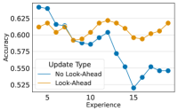
The look-ahead mechanism enables a more accurate calculation of the gradients for the hypernetwork. Here, we show that applying look-ahead-based updates can be beneficial, especially for ResNet-, without significantly increasing computation time. In Table 4, we compare partial HNs with and without look-ahead updates for different versions of ResNet- for the same random seed and class order in the stream. The results show that in most cases, the look-ahead update improves the ACA at the end of the stream. Furthermore, we visualize the test accuracy for experiences to in a random run for both update modes in Figure 11. The visualizations indicate that except for the second, in the rest of the experiences, the strategy with look-ahead update performs overall better.


| Model | Update Type | ACA | Learning Accuracy | Running Time |
| ResNet- | No Look-Ahead | Min | ||
| Look-Ahead | Min | |||
| ResNet- | No Look-Ahead | Min | ||
| Look-Ahead | Min | |||
| ResNet- | No Look-Ahead | Min | ||
| Look-Ahead | Min | |||
| ResNet- | No Look-Ahead | Min | ||
| Look-Ahead | Min | |||
| ResNet- | No Look-Ahead | Min | ||
| Look-Ahead | Min | |||
B.2 First Order vs. Second-Order
Since the computation of the second-order derivatives can be computationally very expensive, we compare both first-order and second-order based estimations of the gradients for the hypernetwork. As demonstrated in Table 5, for some model versions, the second-order estimation can be slightly better, while in others, the first-order can even perform better in terms of ACA. However, the running time for the second-order is significantly longer. Therefore, considering the huge gap in the running time, a first-order estimation is a more reasonable choice.
| Model | Update Type | ACA | Learning Accuracy | Running Time |
| ResNet- | First-Order | Min | ||
| Second-Order | Min | |||
| ResNet- | First-Order | Min | ||
| Second-Order | Min | |||
| ResNet- | First-Order | Min | ||
| Second-Order | Min | |||
| ResNet- | First-Order | Min | ||
| Second-Order | Min | |||
| ResNet- | First-Order | Min | ||
| Second-Order | Min | |||
Appendix C Memory Usage
In this section we compare the memory usage between different versions of latent replay and partial hypernetworks in Table 6. For LR, the memory usage is calculated for the exemplars stored in the replay buffer, and for HN, the memory usage is equal to the size of the hypernetwork since we need to store the converged hypernetwok from the previous experience for computing the regularization term in the new experience. We assume -bit tensors in our calculations.
The memory usage for exemplars in LR is affected by both increasing the size of the input and changing the architecture, in particular by changing the number of channels in a convolutional neural network. In HN, the memory usage is determined by the size of the main network, which can be reduced by partially generating the weights of the main model.
| Latent Replay | Partial Hypernetwork | ||||||
| Model | Exemplar Shape | Memory Usage | Model | # of HN Parameters | Memory Usage | ||
| CIFAR-100 | LR-0 | MB | HN-F | MB | |||
| LR-1 | MB | HN-1 | MB | ||||
| LR-2 | MB | HN-2 | MB | ||||
| LR-3 | MB | HN-3 | MB | ||||
| LR-4 | MB | HN-4 | MB | ||||
| Model | Exemplar Shape | Memory Usage | Model | # of HN Parameters | Memory Usage | ||
| TinyImageNet | LR-0 | MB | HN-F | MB | |||
| LR-1 | MB | HN-1 | MB | ||||
| LR-2 | MB | HN-2 | MB | ||||
| LR-3 | MB | HN-3 | MB | ||||
| LR-4 | MB | HN-4 | MB | ||||
Appendix D Algorithm
In Algorithm 1 we present the steps for training a partial hypernetwork over a CL stream.
Appendix E Gradient Similarity
In Figure 12 we demonstrate the cosine similarity of the hypernetwork gradients (from the cross-entropy loss) and (from the virtual update) in HN-4, as computed in Algorithm 1 in the first epoch of the second experience. The plots show negative similarity regardless of the class order or the model initialization which are affected by the random seeds.

Appendix F Hyperparameter Selection
We carried out a hyper-parameter selection at the stream level. For common hyper-parameters like learning rate, we implemented a grid search and assessed the model’s final performance on the test set of each stream across three runs (using 3 random seeds). In our experiments, we used a learning rate of for both models.
For the hypernetwork, we executed a grid-search, opting for the minimum embedding size capable of attaining a similar performance. This approach allowed us to minimize the hypernetwork’s number of parameters. In our experiments, we used dimension sizes , , and for the embedding dimension the three consecutive layers of the multi-layer peceptron respectively. We set the hypernetwork’s regularization coefficient to .