Parameter estimation and long-range dependence of the fractional binomial process
Meena Sanjay Babulal∗a, Sunil Kumar Gauttam∗b and Aditya Maheshwari#ca[email protected], b[email protected], c[email protected]∗Department of Mathematics, The LNM Institute of Information Technology, Rupa ki Nangal, Post-Sumel, Via-Jamdoli
Jaipur 302031,
Rajasthan, India.
#Operations Management and Quantitative Techniques Area,
Indian Institute of Management Indore, Indore 453556, Madhya Pradesh, India.
Abstract.
In 1990, Jakeman (see [21]) defined the binomial process as a special case of the classical birth-death process, where the probability of birth is proportional to the difference between a fixed number and the number of individuals present.
Later, a fractional generalization of the binomial process was studied by Cahoy and Polito (2012) (see [7]) and called it as fractional binomial process (FBP). In this paper, we study second-order properties of the FBP and the long-range behavior of the FBP and its noise process. We also estimate the parameters of the FBP using the method of moments procedure. Finally, we present the simulated sample paths and its algorithm for the FBP.
A linear birth and death process, introduced by Feller (see [18]), is widely used to model population dynamics (see [2, 3, 38]), queuing systems (see [19]), and other phenomena (see [11, 35, 43]) in which entities enter and exit a system over time. In population model, individuals give birth to new individual with the rate and individuals die with rate , independent of each other.
Several researchers have studied its statistical properties (see [10, 14, 25, 26, 42]), and there are numerous domains in which it finds use, including biology (see [39, 45]), ecology (see [2, 11, 12]),
and finance (see [27, 28, 41]).
Jakeman (see [21]) studied a linear birth and death process in which the birth rate is proportional to
, where is a fixed large number and is present population,
while
the mortality rate stays linear in . Moreover, it is demonstrated that an equilibrium with a binomial distribution is attained as time tends to infinity, and therefore it is called the binomial process. The behavior of the binomial process differs from that of the traditional linear birth-death process, since in the binomial process the birth rate is proportional to
makes chances of birth equal to zero whenever population size reaches . Therefore, population never crosses size in the binomial process, whereas no such restriction of upper bound on population size in the classical linear birth and death process exists. The binomial process has found its application in several areas, such as, the telegraph wave models (see [1, 23]), quantum optics (see [15, 24, 13]), and etc.
Recently, the fractional binomial process (FBP) ,
was introduced by Cahoy and
Polito (see [7]), with birth rate and death rate . It is obtained by taking the fractional-order derivative in place of the integer order derivative in the governing differential equation of the
binomial process. They also showed that one dimensional distribution of the FBP is same as the binomial process subordinated by inverse -stable subordinator, .
It preserves the binomial limit when time tends to infinity which makes it appealing for application in areas such as quantum optics (see [22])
and several other disciplines (see [20, 33, 44]).
Cahoy and
Polito (see [7]) have studied several statistical properties of the FBP such as mean, variance, extinction probability and state probability. The second order properties of the FBP still remains to be investigated and one of them is the long-range dependence (LRD) property. The LRD property of a
stochastic model or a process refers to the presence
of long-term persistence of autocorrelation over time. More
specifically, it means that the autocorrelation
function of the process decays slowly, indicating that distant observations are
still not uncorrelated.
This property is in contrast to short-range
dependence (SRD) property, where correlation decay quickly as
the lag between observations increase.
The LRD property has found use-cases in several sub-domains like modeling, prediction, and risk management. One can find its applications in various fields, including finance (see [31, 33]), climate science (see [44]), biomedical engineering (see [20, 37]), econometrics (see [36]), etc.
In this paper, we
prove that the FBP has the LRD
property. Let be fixed, the increments of the FBP
are defined as:
which we call the fractional binomial noise (FBN). We prove that the FBN has the SRD property.
Parameter estimation is a fundamental aspect of data analysis, where the goal is to determine the values of unknown parameters in a model or system based on observed data.
The parameter estimation of the the FBP is not known in the literature and in this paper we discuss the same using the method of moments. The simulated sample paths of the FBP gives an visual idea of the evolution of the process and in this paper we present simulated sample paths for the FBP.
The subsequent sections of the paper are structured as follows. In Section 2, we have stated some preliminary results regarding the binomial process
and the FBP. Section 3 deals with the LRD property of the FBP and the SRD property of the FBN. Section 4 presents different simulation algorithms to create the sample path of the FBP. Finally, in Section 5, we have studied the parameter estimation for the FBP.
2. Preliminaries
In this section, we introduce some notations, definitions and results that will be used later. A linear birth-and-death (LBD) process is a
continuous-time Markov chain (CTMC),
, defined on the countable state
space and, the transitions
are permitted only to its nearest neighbours.
The state probability of LBD satisfies following Cauchy problem (see [3])
(2.1)
where, is the initial population. An LBD process have applications in several areas, such as, modelling population dynamics (see [2, 3, 38]), queuing systems (see [19]) and biological systems (see [39, 45, 2, 11, 12]).
Jakeman (see [21]) studied linear birth and death process with some modifications and obtained the binomial process. We next present some preliminary results of the binomial process that will be needed later in this paper.
2.1. Binomial process
Jakeman (see [21]) introduced the classical binomial process with birth rate and death rate has initial value problem for the state probability given by
(2.2)
where , is the initial population and is the maximum attainable population.
The state space of the binomial process is . The
generating function for is defined as
and it satisfies the following partial differential equation (pde)
(2.3)
where is the initial number of individuals and . The solution of the above equation (2.3) is given by
(2.4)
where and
The joint probability generating function of the binomial process is given as (see [21] )
(2.5)
where is given by (2.4) and the subscript denotes the initial population. The probability of finding individuals given by (see [21])
(2.6)
Moreover, it is observed in [21] that as time tends to infinity, the evolving population follows a binomial distribution with parameters and
We now state some preliminary results of the FBP that will be needed later.
2.2. Fractional Binomial process
The FBP (see [7]) is obtained by taking fractional-order derivative in place of the integer-order derivative in the governing differential equation of the binomial process given in (2.2). The governing differential equation of the FBP with birth rate and death rate is given by
(2.7)
The inverse -stable subordinator is defined as the right-continuous of the -stable subordinator (see [6, 34])
It is observed (see [7]) that the one-dimensional distribution of the FBP can be written as time-changed binomial process by an independent inverse -stable subordinator ,
i.e.,
(2.8)
where and
It is known that (see [7]) the generating function of the FBP solves the following differential equation
(2.9)
where the initial number of individuals is , and .
Definition 2.1.
Let and be two functions, then they are called asymptotically equivalent denoted by , if
The Mittag–Leffler function can be defined as (see [17])
Now, using expansion of , where (see [5]), we will show that asymptotically equivalent to ,
that is
(2.10)
The mean and variance of the FBP are
given by (see [7] )
(2.11)
(2.12)
where is the Mittag–Leffler function.
2.3. The long and short range dependence
In the literature, there are various definitions of the LRD and SRD characteristics of a stochastic process. However, for the purpose of this paper, we will utilize the following definition (see [4, 16, 32]) for non stationary process.
Definition 2.2.
Let and be a stochastic process and the asymptotic behaviour of its correlation function is given by
for fixed and .
Then, we say that the stochastic process has the LRD property if , otherwise it is said to have the SRD property when .
3. Dependence structure for the FBP
The aim of this section is to examine the LRD and SRD property of the FBP and the fractional binomial noise (FBN) respectively. Now, we derive some results which are needed to prove it. First, we derive the recurrence relation for the joint probability generating function (pgf) of the FBP.
Lemma 3.1.
The joint pgf of the FBP satisfies the following relationship
(3.1)
where is given by (2.6)
and is the solution of (2.9) with initial population .
Proof.
Let denote the probability of finding individuals present at time and individuals at time
, and is given by
(3.2)
Now, we have the generating function for the FBP as
Let be fixed, and define the
increments of the fractional binomial process as the fractional binomial noise (FBN) is
The noise process find applications in sonar communication (see [40]), vehicular communications (see [30]), wireless sensor networks (see [29]) and many other fields, where signals are transmitted through noise. We now explore the dependence structure of the fractional binomial noise (FBN) .
In this section, we provide algorithm to simulate the FBP, which we will use in Section 5 for parameter estimation of the FBP.
The sojourn time of the process is defined as the duration for which it remains in current state .
The distribution of sojourn or inter-arrival time is given by (see [38, Chapter VI, Section 3.2])
and thus the pdf of the sojourn time is given by
Using (2.8), we obtain the sojourn time,
for the FBP as given below
This implies that the FBP changes state from to or with probability or respectively. Now, it can be simulated using the following procedure.
Algorithm 1 Simulation of the fractional binomial process
0: , , , and
.
0: , simulated sample paths for the fractional binomial process.
Initialisation : is present population where , is desired number of birth or death occurs and is fixed large number.
1:fordo
2: generate a negatively exponentially distributed random variable and a one sided -stable random variable .
3: simulate .
4:ifthen
5:
6: otherwise
7:endif
8:endfor
9:return
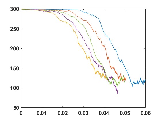
(a) , , , ,
(b) , , , ,
Figure 1. Five simulated sample path of binomial and fractional binomial process
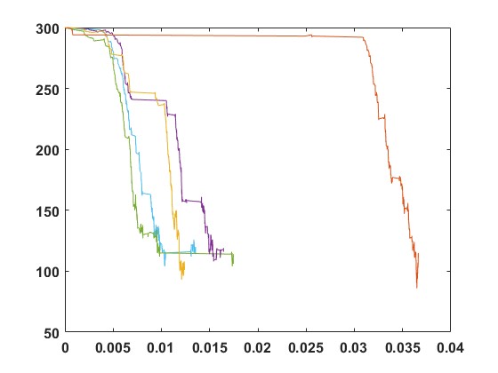
(a) , , , ,
(b) , , , ,
Figure 2. Five simulated sample path of the fractional binomial process
Interpretation of the sample paths
We observe from Figure 1 that when we compare the binomial process with the FBP a sudden population burst (negative burst due to higher death rate) is visible in the FBP, that is, the population burst frequency increases as we decreases value of from to . The sample paths of the FBP in Figure 1- 2 keeps revolving around their theoretical mean.
5. Parameter estimation of the FBP
The method of moments (MoM) is a statistical technique used for estimating the parameters of the distribution of a population. The moments are summary statistics that describe various aspects of the distribution, such as mean, variance, skewness, and kurtosis. Here, we have not used maximum likelihood estimator technique as there is no explicit expression of density of the FBP is available. We can not use linear regression model for parameter estimation used by Cahoy and Polito used in ( see [8, 9]) as our model is non-linear regression model.
Let be fixed time and denotes the value obtained by simulating sample paths of the FBP. Then, using we evaluate sample mean () and sample second moment ( as follows
(5.1)
We denote the population first moment by (as a function of and, and the population second moment by then using (2.11) and (2.2), we get
(5.2)
(5.3)
To estimate parameter and , we equate sample moments of the FBP (5.1) with the population moments (5.2) and numerically solve the following equation
(5.4)
We took sample and repeated this process times, while estimating parameters, that is,
we generate this samples of the FBP for different sample sizes , and
Then, we evaluate sample mean () and sample second moment ( using (5) for , which gives
estimates of and each from above equation (5), subsequently, we take average of estimates of and to obtain and .
Here, we have used numerical method to solve equations (5) as it is easy to observe from equation (5.2) that they have complicated form and hard to solve analytically. The tables below display these values together with associated MAD (mean absolute deviation) and MSE (mean square error). For five distinct pairs of values of and , the FBP data were simulated.
Table 1. Parameter estimation and its dispersion’s of the FBP for parameter and
with , and .
MeanMADMSE
MeanMADMSE
MeanMADMSE
0.3045
0.0071
0.000073
0.3036
0.0046
0.00003
0.3016
0.0018
0.00001
0.8652
0.1853
0.0482
0.8588
0.1820
0.0466
0.8358
0.0547
0.0042
Table 2. Parameter estimation and its dispersion’s of the FBP for parameter and with , and .
MeanMADMSE
MeanMADMSE
MeanMADMSE
0.4942
0.0177
0.00049
0.4962
0.0060
0.00006
0.4975
0.0078
0.00009
0.4395
0.0754
0.0090
0.4206
0.0266
0.0011
0.4175
0.0311
0.0017
Table 3. Parameter estimation and its dispersion’s of the FBP for
parameter and with , and .
MeanMADMSE
MeanMADMSE
MeanMADMSE
0.5982
0.0141
0.00005
0.5985
0.0042
0.00003
0.5989
0.0012
0.00001
0.9062
0.0934
0.0156
0.8930
0.0290
0.0013
0.8938
0.0071
0.00008
Table 4. Parameter estimation and its dispersion’s of the FBP for
parameter and
with , and .
MeanMADMSE
MeanMADMSE
MeanMADMSE
0.6845
0.0157
0.00031
0.6874
0.0029
0.000012
0.6804
0.0009
0.00001
0.1405
0.0595
0.00025
0.1479
0.0521
0.000012
0.1501
0.0020
0.000005
Table 5. Parameter estimation and its dispersion’s of the FBP for parameter and with , and .
MeanMADMSE
MeanMADMSE
MeanMADMSE
0.8877
0.0254
0.0010
0.8896
0.0095
0.00014
0.8902
0.0028
0.00001
0.5383
0.0954
0.0095
0.5221
0.0207
0.00008
0.5209
0.0070
0.00007
The estimation Tables 15 demonstrate that the relative fluctuation for estimates of and keep approaching true value as sample sizes increase. We also observe that the true value of parameters and estimated parameters are very close to each other and there is nearly less than percent of variation between them. It is important to keep in mind that typical sample size in many real-world applications, including network traffic data, are in the millions or more. Given the context and calculations done, we claim that our results shows robust and accurate parameter estimation. Table 6 shows result for percent bias and coefficient of variation (CV) based on for simulation, where
Percent bias
CV
Table 6. Percent bias and coefficient of variation for parameter and
()
Bias
CV
Bias
CV
Bias
CV
1.5146
2.8224
1.2027
1.8942
0.7977
0.7985
8.1469
25.8868
7.3469
23.4176
4.4778
7.8188
1.1597
5.0131
0.7068
4.5306
0.7011
1.5336
9.8809
23.6730
9.4664
21.4996
5.1618
8.0970
0.3976
2.8965
0.3026
0.8610
0.2382
0.2425
4.0488
13.8720
0.7369
4.1093
0.6852
1.0077
2.2198
2.7068
1.8022
0.5726
1.3710
0.1674
29.7280
11.8007
26.0687
2.8390
25.7242
1.6509
1.3624
3.5978
1.1550
1.3553
1.1537
0.3964
13.2784
18.2131
12.9863
5.112
10.2784
1.7249
Concluding Remarks
We have investigated that the FBP has the LRD property and its increment exhibits the SRD property. We have used the one-dimensional distributions of the FBP to simulate sample path for the process. We have derived the distribution of sojourn time of the FBP and used it to simulate sample trajectories. We have used MoM estimation technique to estimate parameters of the FBP. On comparing generated sample path in Figure 1, we can see that time taken to occur next birth or death reduces and population burst occurs. This behaviour makes the FBP more applicable in nature as such incidences occurs in real life, for example during Covid- demand of masks, sanitizer, oxygen cylinder and many other things saw a burst in their demands.
First author would like to acknowledge the Centre for Mathematical & Financial Computing
and the DST-FIST grant for the infrastructure support for the computing
lab facility under the scheme FIST (File No: SR/FST/MS-I/2018/24)
at the LNMIIT, Jaipur.
References
[1]
David middleton, an introduction to statistical communication theory,
mcgraw-hill, 1961.
[2]
Jean Avan, Jean Avan, Nicolas Grosjean, Nicolas Grosjean, Thierry Huillet, and
Thierry Huillet.
Did the ever dead outnumber the living and when? a birth-and-death
approach.
Physica A-statistical Mechanics and Its Applications, 2015.
[3]
Norman T. J. Bailey.
The elements of stochastic processes with applications to the
natural sciences.
John Wiley & Sons, Inc., New York-London-Sydney, 1964.
[4]
Luisa Beghin and Costantino Ricciuti.
Lévy processes linked to the lower-incomplete gamma function.
Fractal and Fractional, 5(3), 2021.
[5]
Mario N Berberan-Santos.
Properties of the mittag-leffler relaxation function.
Journal of Mathematical Chemistry, 38(4):629–635, 2005.
[6]
N. H. Bingham.
Limit theorems for occupation times of Markov processes.
Z. Wahrscheinlichkeitstheorie und Verw. Gebiete, 17:1–22,
1971.
[7]
Dexter O Cahoy and Federico Polito.
On a fractional binomial process.
Journal of Statistical Physics, 146:646–662, 2012.
[8]
Dexter O. Cahoy and Federico Polito.
Parameter estimation for fractional birth and fractional death
processes.
Stat. Comput., 24(2):211–222, 2014.
[9]
Dexter O Cahoy, Federico Polito, and Vir Phoha.
Transient behavior of fractional queues and related processes.
Methodology and Computing in Applied Probability, 17:739–759,
2015.
[10]
Rui Chen, Ollivier Hyrien, Rui Chen, Rui Chen, and Ollivier Hyrien.
Quasi- and pseudo-maximum likelihood estimators for discretely
observed continuous-time markov branching processes.
Journal of Statistical Planning and Inference, 2011.
[11]
Cláudia Codeço, Subhash Lele, Mercedes Pascual, Menno Bouma, and Albert Ko.
A stochastic model for ecological systems with strong nonlinear
response to environmental drivers: Application to two water-borne diseases.
Journal of the Royal Society, Interface / the Royal Society,
5:247–52, 08 2007.
[12]
Miklós Csűrös and István Miklós.
A probabilistic model for gene content evolution with duplication,
loss, and horizontal transfer.
10 2005.
[13]
Wilbur B. Davenport and William L. Root.
An introduction to the theory of random signals and noise.
1958.
[14]
A. C. Davison, Anthony C. Davison, Sophie Hautphenne, Sophie Hautphenne, Andrea
Kraus, and Andrea Kraus.
Parameter estimation for discretely observed linear birth-and-death
processes.
Biometrics, 2020.
[15]
P. Diament, Paul Diament, Malvin C. Teich, and Malvin C. Teich.
Evolution of the statistical properties of photons passed through a
traveling-wave laser amplifier.
IEEE Journal of Quantum Electronics, 1992.
[16]
Mirko D’Ovidio and Erkan Nane.
Time dependent random fields on spherical non-homogeneous surfaces.
Stochastic Processes and their Applications, 124(6):2098–2131,
2014.
[17]
Arthur Erdelyi, Wilhelm Magnus, Fritz Oberhettinger, and Francesco G. Tricomi,
editors.
Higher transcendental functions: Vol 2.
California Institute of Technology Bateman manuscript project.
McGraw-Hill, New York, 1953.
[18]
William Feller and William Feller.
Die grundlagen der volterraschen theorie des kampfes ums dasein in
wahrscheinlichkeitstheoretischer behandlung.
Acta Biotheoretica, 1939.
[19]
Willliam Feller.
An introduction to probability theory and its applications, vol
2.
John Wiley & Sons, 2008.
[20]
Plamen Ch Ivanov, Luis A Nunes Amaral, Ary L Goldberger, Shlomo Havlin,
Michael G Rosenblum, Zbigniew R Struzik, and H Eugene Stanley.
Multifractality in human heartbeat dynamics.
Nature, 399(6735):461–465, 1999.
[21]
E Jakeman.
Statistics of binomial number fluctuations.
Journal of Physics A: Mathematical and General, 23(13):2815,
1990.
[22]
E. Jakeman and E Jakeman.
Non-gaussian statistical models for scattering calculations.
Waves in Random Media, 1991.
[23]
E. Jakeman, E Jakeman, R. Loudon, and R Loudon.
Fluctuations in quantum and classical populations.
Journal of Physics A, 1991.
[24]
E. Jakeman, Eric Jakeman, Eric Jakeman, Sean Phayre, Sean Phayre, Eric Renshaw,
and Eric Renshaw.
The evolution and measurement of a population of pairs.
Journal of Applied Probability, 1995.
[25]
Niels Keiding and Niels Keiding.
Maximum likelihood estimation in the birth-and-death process.
Advances in Applied Probability, 1974.
[26]
David G. Kendall.
Stochastic Processes and Population Growth.
Journal of the Royal Statistical Society: Series B
(Methodological), 11(2):230–264, 12 2018.
[27]
S. C. Kou and S. C. Kou.
Modeling growth stocks via birth-death processes.
Advances in Applied Probability, 2003.
[28]
Samuel Kou and Steven Kou.
Modeling growth stocks via size distribution.
SSRN Electronic Journal, 11 2001.
[29]
Iratxe Landa, Aitor Blazquez, Manuel Velez, and Amaia Arrinda.
Indoor measurements of iot wireless systems interfered by impulsive
noise from fluorescent lamps.
pages 2080–2083, 03 2017.
[30]
Sicong Liu, Fang Yang, Wenbo Ding, and Jian Song.
Double kill: Compressive-sensing-based narrow-band interference and
impulsive noise mitigation for vehicular communications.
IEEE Transactions on Vehicular Technology, 65:1–1, 01 2015.
[31]
Thomas Lux.
The stable paretian hypothesis and the frequency of large returns: an
examination of major german stocks.
Applied financial economics, 6(6):463–475, 1996.
[32]
A. Maheshwari and P. Vellaisamy.
On the long-range dependence of fractional poisson and negative
binomial processes.
Journal of Applied Probability, 53(4):989–1000, 2016.
[33]
Benoit Mandelbrot.
The variation of certain speculative prices.
J. Bus., 36(4):394, January 1963.
[34]
M. M. Meerschaert and P. Straka.
Inverse stable subordinators.
Math. Model. Nat. Phenom., 8(2):1–16, 2013.
[35]
Sean Nee.
Birth-death models in macroevolution. ann rev ecol evol s.
Annu. Rev. Ecol. Evol. Syst, 37:1–17, 12 2006.
[36]
Adrian Pagan.
The econometrics of financial markets.
Journal of empirical finance, 3(1):15–102, 1996.
[37]
C-K Peng, Shlomo Havlin, H Eugene Stanley, and Ary L Goldberger.
Quantification of scaling exponents and crossover phenomena in
nonstationary heartbeat time series.
Chaos: an interdisciplinary journal of nonlinear science,
5(1):82–87, 1995.
[38]
Mark Pinsky and Samuel Karlin.
An introduction to stochastic modeling.
Academic press, 2010.
[39]
Mary Sehl, Hua Zhou, Janet S. Sinsheimer, and Kenneth L. Lange.
Extinction models for cancer stem cell therapy.
Mathematical Biosciences, 234(2):132–146, 2011.
[40]
Milica Stojanovic and J. Preisig.
Underwater acoustic communication channels: Propagation models and
statistical characterization.
Communications Magazine, IEEE, 47:84 – 89, 02 2009.
[41]
Hiroya Takada, Hideyuki Takada, Ushio Sumita, Ushio Sumita, Hui Jin, and Hui
Jin.
Development of computational algorithms for evaluating option prices
associated with square-root volatility processes.
Methodology and Computing in Applied Probability, 2009.
[42]
Simon Tavaré and Simon Tavaré.
The linear birth‒death process: an inferential retrospective.
Advances in Applied Probability, 2018.
[43]
Jeffrey Thorne, Hirohisa Kishino, and J. Felsenstein.
Erratum: An evolutionary model for maximum likelihood alignment of
dna sequences (j mol evol (1991) 33 (114-124)).
Journal of Molecular Evolution, 34:91–92, 01 1992.
[44]
C. Varotsos and D. Kirk-Davidoff.
Long-memory processes in ozone and temperature variations at the
region 60s-60n.
Atmospheric Chemistry and Physics, 6(12):4093–4100, 2006.
[45]
Jason Xu, Peter Guttorp, Midori Kato-Maeda, and Vladimir N. Minin.
Likelihood-based inference for discretely observed
birth–death-shift processes, with applications to evolution of mobile
genetic elements.
Biometrics, 71(4):1009–1021, 2015.