Parameter calibration with Consensus-based Optimization for interaction dynamics driven by neural networks

In the following we consider feed-forward artificial neural networks of the form

Note that the output layer has no bias unit. The entry $\theta_{j,k}^{\ell}$ of the weight matrix $\theta^{(\ell)}\in\mathbb{R}^{n^{(\ell-1)}\times n^{(\ell)}}$ describes the weight from neuron $a_{j}^{(\ell-1)}$ to the neuron $a_{k}^{(\ell)}$. For notational convenience, we assemble all entries $\theta_{j,k}^{(\ell)}$ in a vector $\mathbb{R}^{K}$ with

$$K:=n^{(1)}\cdot n^{(2)}+n^{(2)}\cdot n^{(3)}+\dots+n^{(L-1)}\cdot n^{(L)}.$$

For the numerical experiment we use $g^{(\ell)}=\log(1+e^{x})$ for $\ell=2,\dots,N-1$ and $g^{(L)}(x)=x.$ For an illustration of the NN structure we refer the interested reader to [4]. In the numerical section we consider an NN with $L=3,$ one input and 5 units in the hidden layer.

We solve the parameter calibration problem with the help of a Consensus-based optimization method [3]. In more details, we choose the variant introduced in [2] which is tailored for high-dimensional problems involving the calibration of neural networks. The CBO dynamics is itself a stochastic interacting particle system with $N_{\text{CBO}}$ agents given by stochastic differential equations (SDEs). The evolution of the agents is influenced by two terms. On the one hand, there is a deterministic term that aims to confine the positions of the agents at a weighted mean. On the other hand, there is a stochastic term that allows for exploration of the state space. The details are the following

(3)

$$du_{t}^{i}=-\lambda(u_{t}^{i}-v_{f})dt+\sigma\text{diag}(u_{t}^{i}-v_{f})dB_{t}^{i},\quad i=1,\dots,N_{\text{CBO}}$$

with drift and diffusion parameters $\lambda,\sigma>0$, independent $d$-dimensional Brownian motions $B_{t}^{i}$ and initial conditions $u_{0}^{i}$ drawn uniformly from the parameter set of interest. A main role plays the weighed mean

$$v_{f}=\frac{1}{\sum_{i=1}^{N_{\text{CBO}}}e^{-J(u_{i})}}\sum_{i=1}^{N_{\text{CBO}}}u_{i}\,e^{-\alpha J(u_{i})}.$$

By its construction, agents with lower cost have more weight in the mean as the ones with higher cost. The parameter $\alpha$ allows to adjust this difference of the weights. For more information on the CBO method and its proof of convergence on the mean-field level we refer the interested reader to [5] and the references therein. As indicated by the notation above, the agents used in the CBO method are different realizations of parameter vectors that we consider for the calibration. For the numerical results NN4 we consider a neural network with $13$ weights, i.e., $\theta\in\mathbb{R}^{13}$. Moreover, we assume the maximal speed $v_{\text{max}}$ as additional parameter. Hence, for fixed $t$ we have for the $i$-th CBO agent $u_{t}^{i}\in\mathbb{R}^{14}.$

The data collection of the ESIMAS project contains vehicle data from 5 cameras that were placed in a $1km$ tunnel section on the German motorway A3 nearby Frankfurt/Main [1]. The data is processed in the exact same way as in [4]. Files with the processed data can be found online¹¹1https://github.com/ctotzeck/NN-interaction.

The SDE which represents the CBO scheme is solved with the scheme proposed in [2]. In particular, we set $dt=0.05,\sigma_{0}=1,\lambda=1$ and the maximal number of time steps to $100.$ The mini-batch size of the CBO scheme is $50$ and we have $100$ CBO agents in total. In each time step we update one randomly chosen mini-batch. The initial values are chosen as follows

$$v_{\text{max}}\sim U([20,40]),\quad L\sim U([0,10])\text{ and }\theta\sim U([-0.5,0.5]^{K}).$$

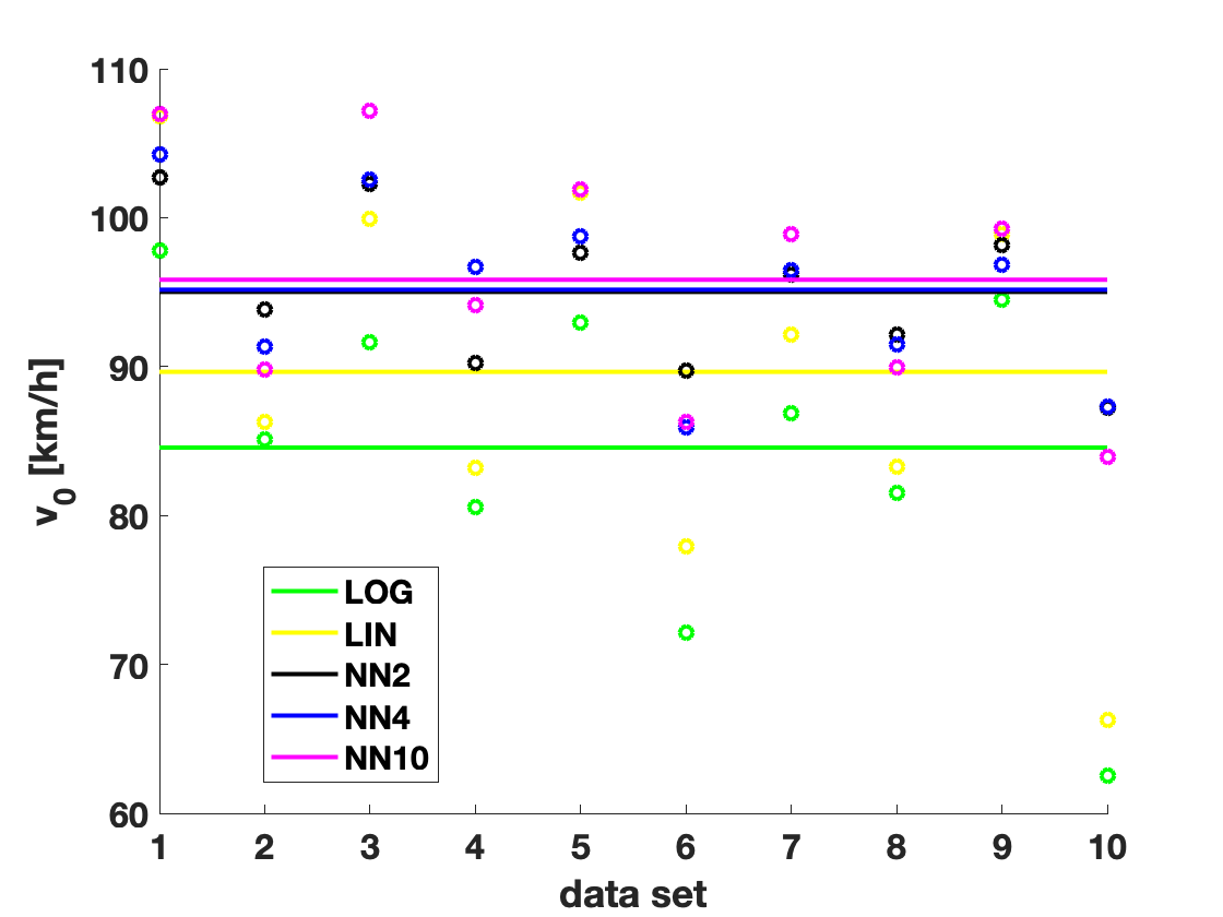
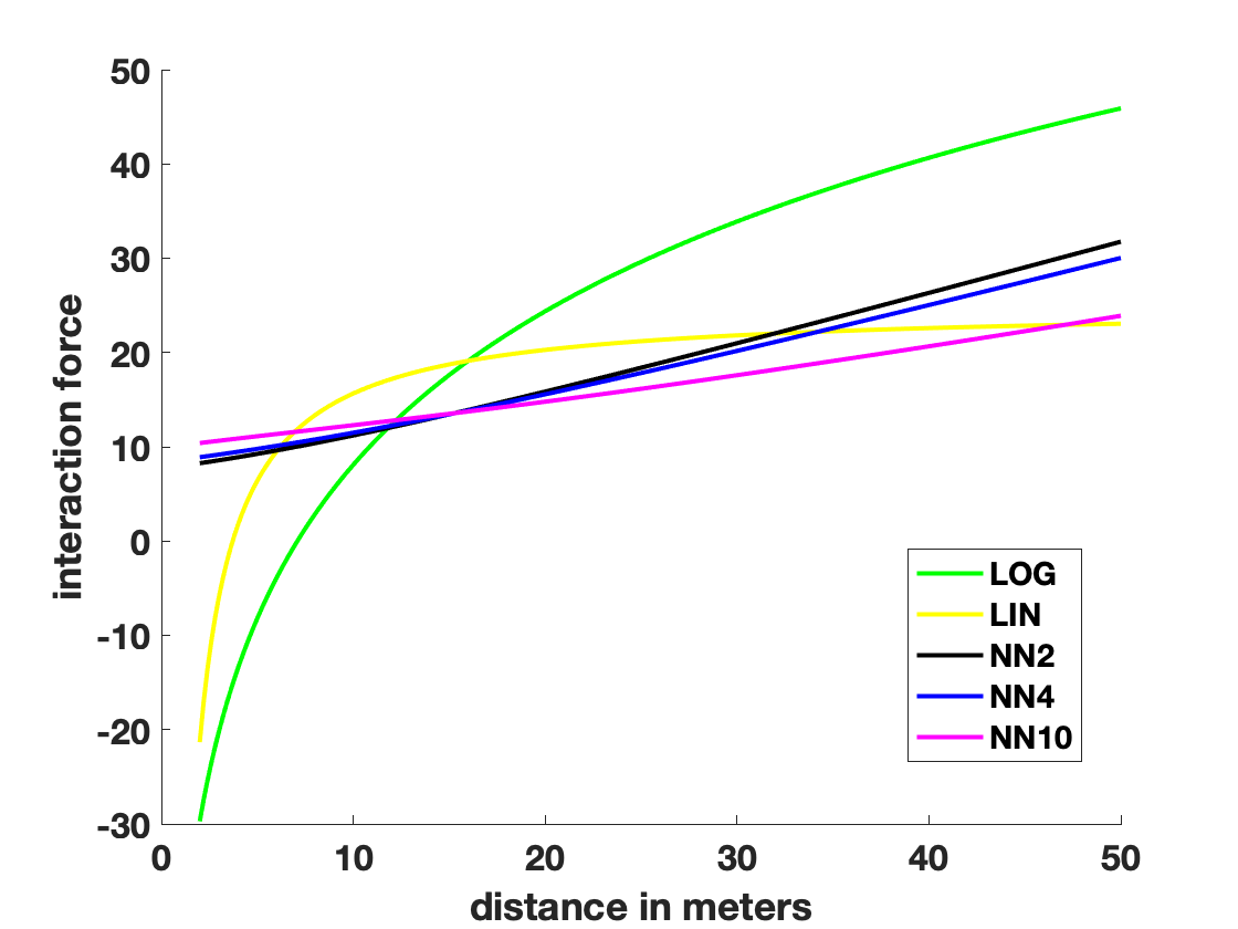
Figure 1 (left) shows the velocities resulting from the parameter calibration process. We find that the estimates velocities for the NN approaches are higher than the velocities of the LWR based models. The difference is most significant in data set $10.$ The plot on the right shows the average of the resulting forces for the different models. The forces of the NN approaches resemble linear approximations of the forces corresponding to the LWR models.

The car length $(L)$ appears only in the LWR models. Its optimized values for the different data sets are given in Table 1. We see that the lengths for the linear model are smaller than the ones in the logarithmic model. This is in agreement with the results obtained with stochastic gradient descent and shown in [4].

Finally, we summarize the cost values after parameter calibration in Table 2. The least values of every column are highlighted. It is obvious that the LWR model with linear force outperforms the other models. The results of the NN approaches are better than the ones of the LWR model with logarithmic force.

References

- [1] S. Lamberty M. Oeser E. Kallo, A. Fazekas. Microscopic traffic data obtained from videos recorded on a german motorway. Mendeley Data 10.17632/tzckcsrpn6.1, 2019.
- [2] L. Li Y. Zhu J. A. Carrillo, S. Jin. A consensus-based global optimization method for high dimensional machine learning problems. ESAIM:COCV, 27(S5), 2021.
- [3] O. Tse S. Martin R. Pinnau, C. Totzeck. A consensus-based model for global optimization and its mean-field limit. Math. Mod. Meth. Appl. Sci., 27(1):183–204, 2017.
- [4] C. Totzeck S. Göttlich. Optimal control for interaction particle systems driven by neural networks. arXiv:2104.01383, 2021.
- [5] C. Totzeck. Trends in consensus-based optimization. arXiv:2104.01383, 2021.