Parallel Longest Increasing Subsequence and
van Emde Boas Trees

Yan Gu UC Riverside [email protected] , Ziyang Men UC Riverside [email protected] , Zheqi Shen UC Riverside [email protected] , Yihan Sun UC Riverside [email protected] and Zijin Wan UC Riverside [email protected]

(2023)

Abstract.

This paper studies parallel algorithms for the longest increasing subsequence (LIS) problem. Let $n$ be the input size and $k$ be the LIS length of the input. Sequentially, LIS is a simple problem that can be solved using dynamic programming (DP) in $O(n\log n)$ work. However, parallelizing LIS is a long-standing challenge. We are unaware of any parallel LIS algorithm that has optimal $O(n\log n)$ work and non-trivial parallelism (i.e., $\tilde{O}(k)$ or $o(n)$ span).

This paper proposes a parallel LIS algorithm that costs $O(n\log k)$ work, $\tilde{O}(k)$ span, and $O(n)$ space, and is much simpler than the previous parallel LIS algorithms. We also generalize the algorithm to a weighted version of LIS, which maximizes the weighted sum for all objects in an increasing subsequence. To achieve a better work bound for the weighted LIS algorithm, we designed parallel algorithms for the van Emde Boas (vEB) tree, which has the same structure as the sequential vEB tree, and supports work-efficient parallel batch insertion, deletion, and range queries.

We also implemented our parallel LIS algorithms. Our implementation is light-weighted, efficient, and scalable. On input size $10^{9}$ , our LIS algorithm outperforms a highly-optimized sequential algorithm (with $O(n\log k)$ cost) on inputs with $k\leq 3\times 10^{5}$ . Our algorithm is also much faster than the best existing parallel implementation by Shen et al. (2022) on all input instances.

^†^†journalyear: 2023^†^†copyright: rightsretained^†^†conference: Proceedings of the 35th ACM Symposium on Parallelism in Algorithms and Architectures; June 17–19, 2023; Orlando, FL, USA^†^†booktitle: Proceedings of the 35th ACM Symposium on Parallelism in Algorithms and Architectures (SPAA ’23), June 17–19, 2023, Orlando, FL, USA^†^†doi: 10.1145/3558481.3591069^†^†isbn: 978-1-4503-9545-8/23/06

1. Introduction

This paper studies parallel algorithms for classic and weighted longest increasing subsequence problems (LIS and WLIS, see definitions below). We propose a work-efficient parallel LIS algorithm with $\tilde{O}(k)$ span, where $k$ is the LIS length of the input. Our WLIS algorithm is based on a new data structure that parallelizes the famous van Emde Boas (vEB) tree (van Emde Boas, 1977). Our new algorithms improve existing theoretical bounds on the parallel LIS and WLIS problem, as well as enable simpler and more efficient implementations. Our parallel vEB tree supports work-efficient batch insertion, deletion and range query with polylogarithmic span.

Given a sequence $A_{1..n}$ and a comparison function on the objects in $A$ , the LIS of $A$ is the longest subsequence (not necessarily contiguous) in $A$ that is strictly increasing (based on the comparison function). In this paper, we use LIS to refer to both the longest increasing subsequence of a sequence, and the problem of finding such an LIS. LIS is one of the most fundamental primitives and has extensive applications (e.g., (Delcher et al., 1999; Gusfield, 1997; Crochemore and Porat, 2010; Schensted, 1961; O’Donnell and Wright, [n. d.]; Zhang, 2003; Altschul et al., 1990; Deift, 2000)). In this paper, we use $n$ to denote the input size and $k$ to denote the LIS length of the input. LIS can be solved by dynamic programming (DP) using the following DP recurrence (more details in Sec. 2).

(1)

\mathit{dp}[i]=\max(1,{\max}_{j<i,A_{j}<A_{i}}\mathit{dp}[j]+1)

Sequentially, LIS is a straightforward textbook problem (Dasgupta et al., 2008; Goodrich and Tamassia, 2015). We can iteratively compute $\mathit{dp}[i]$ using a search structure to find ${\max}_{j<i,A_{j}<A_{i}}\mathit{dp}[j]$ , which gives $O(n\log n)$ work. However, in parallel, LIS becomes challenging both in theory and in practice. In theory, we are unaware of parallel LIS algorithms with $O(n\log n)$ work and non-trivial parallelism ( $o(n)$ or $\tilde{O}(k)$ span). In practice, we are unaware of parallel LIS implementations that outperform the sequential algorithm on general input distributions. We propose new LIS algorithms with improved work and span bounds in theory, which also lead to a more practical parallel LIS implementation.

Our work follows some recent research (Blelloch et al., 2012b, a; Fischer and Noever, 2018; Hasenplaugh et al., 2014; Pan et al., 2015; Shun et al., 2015; Blelloch et al., 2020c, 2018, d; Gu et al., 2022b; Shen et al., 2022; Blelloch et al., 2020b) that directly parallelizes sequential iterative algorithms. Such algorithms are usually simple and practical, given their connections to sequential algorithms. To achieve parallelism in a “sequential” algorithm, the key is to identify the dependences (Shun et al., 2015; Blelloch et al., 2020c, d; Shen et al., 2022) among the objects. In the DP recurrence of LIS, processing an object $x$ depends on all objects $y<x$ before it, but does not need to wait for objects before it with a larger or equal value.

An “ideal” parallel algorithm should process all objects in a proper order based on the dependencies—it should 1) process as many objects as possible in parallel (as long as they do not depend on each other), and 2) process an object only when it is ready (all objects it depends on are finished) to avoid redundant work. More formally, we say an algorithm is round-efficient (Shen et al., 2022) if its span is $\tilde{O}(D)$ for a computation with the longest logical dependence length $D$ . In LIS, the logical dependence length given by the DP recurrence is the LIS length $k$ . We say an algorithm is work-efficient if its work is asymptotically the same as the best sequential algorithm. Work-efficiency is crucial in practice, since nowadays, the number of processors on one machine (tens to hundreds) is much smaller than the problem size. A parallel algorithm is less practical if it significantly blows up the work of a sequential algorithm.

Unfortunately, there exists no parallel LIS algorithm with both work-efficiency and round-efficiency. Most existing parallel LIS algorithms are not work-efficient (Galil and Park, 1994; Krusche and Tiskin, 2009; Semé, 2006; Thierry et al., 2001; Nakashima and Fujiwara, 2002, 2006; Krusche and Tiskin, 2010; Shen et al., 2022), or have $\tilde{\Theta}(n)$ span (Alam and Rahman, 2013). We review more related work in Sec. 7.

Our algorithm is based on the parallel LIS algorithm and the phase-parallel framework by Shen et al. (Shen et al., 2022). We refer to it as the SWGS algorithm, and review it in Sec. 2. The phase-parallel framework defines a rank for each input object as the length of LIS ending at it (the $\mathit{dp}$ value in Eq. 1). Note that an object only depends on lower-rank objects. Hence, the phase-parallel LIS algorithm processes all objects based on the increasing order of ranks. However, the SWGS algorithm takes $O(n\log^{3}n)$ work whp, $\tilde{O}(k)$ span, and $O(n\log n)$ space, and is quite complicated. In the experiments, the overhead in work and space limits the performance. On a 96-core machine and input size of $10^{8}$ , SWGS becomes slower than a sequential algorithm when the LIS length $k>100$ .

In this paper, we propose a parallel LIS algorithm that is work-efficient ( $O(n\log k)$ work), round-efficient ( $\tilde{O}(k)$ span) and space-efficient ( $O(n)$ space), and is much simpler than previous parallel LIS algorithms (Shen et al., 2022; Krusche and Tiskin, 2010). Our result is summarized in Thm. 1.1.

Theorem 1.1 (LIS).

Given a sequence $A$ of size $n$ and LIS length $k$ , the longest increasing subsequence (LIS) of $A$ can be computed in parallel with $O(n\log k)$ work, $O(k\log n)$ span, and $O(n)$ space.

We also extend our algorithm to the weighted LIS (WLIS) problem, which has a similar DP recurrence as LIS but maximizes the weighted sum instead of the number of objects in an increasing subsequence.

(2)

\mathit{dp}[i]=w_{i}+\max(0,{\max}_{j<i,A_{j}<A_{i}}\mathit{dp}[j])

where $w_{i}$ is the weight of the $i$ -th input object. We summarize our result in Thm. 1.2.

Theorem 1.2 (WLIS).

Given a sequence $A$ of size $n$ and LIS length $k$ , the weighted LIS of $A$ can be computed using $O(n\log n\log\log n)$ work, $O(k\log^{2}n)$ span, and $O(n\log n)$ space.

Our primary techniques to support both LIS and WLIS rely on better data structures for 1D or 2D prefix min/max queries in the phase-parallel framework. For the LIS problem, our algorithm efficiently identifies all objects with a certain rank using a parallel tournament tree that supports 1D dynamic prefix-min queries, i.e., given an array of values, find the minimum value for each prefix of the array. For WLIS, we design efficient data structures for 2D dynamic “prefix-max” queries, which we refer to as dominant-max queries (see more details in Sec. 4). Given a set of 2D points associated with values, which we refer to as their scores, a dominant-max query returns the largest score to the bottom-left of a query point. Using dominant-max queries, given an object $x$ in WLIS, we can find the maximum $\mathit{dp}$ value among all objects that $x$ depends on. We propose two solutions focusing on theoretical and practical efficiency, respectively. In practice, we use a parallel range tree similar to that in SWGS, which results in $O(n\log^{2}n)$ work and $\tilde{O}(k)$ span for WLIS. In theory, we parallelize the van Emde Boas (vEB) tree (van Emde Boas, 1977) and integrate it into range trees to achieve a better work bound for WLIS.

Refer to caption — Figure 1. Outline and contributions of this paper.

The van Emde Boas (vEB) tree (van Emde Boas, 1977) is a famous data structure for priority queues and ordered sets on integer keys, and is introduced in many textbooks (e.g., (Cormen et al., 2009)). To the best of our knowledge, our algorithm is the first parallel version of vEB trees. We believe our algorithm is of independent interest in addition to the application in WLIS. We note that it is highly non-trivial to redesign and parallelize vEB trees because the classic vEB tree interface and algorithms are inherently sequential. Our parallel vEB tree supports a general ordered set abstract data type on integer keys in $[0,U)$ with bounds stated below. We present more details in Sec. 5.

Theorem 1.3 (Parallel vEB Tree).

Let $\mathcal{U}$ be a universe of all integers in range $[0,U)$ . Given a set of integer keys from $\mathcal{U}$ , there exists a data structure that has the same organization as the sequential vEB tree, and supports:

•

single-point insertion, deletion, lookup, reporting the minimum (maximum) key, and reporting the predecessor and successor of an element, all in $O(\log\log U)$ work, using the same algorithms for sequential vEB trees;
•

BatchInsert $(B)$ and BatchDelete $(B)$ that insert and delete a sorted batch $B\subseteq\mathcal{U}$ in the vEB tree with $O(|B|\log\log U)$ work and $O(\log U)$ span;
•

Range $(k_{L},k_{R})$ that reports all keys in range $[k_{L},k_{R}]$ in $O((1+m)\log\log U)$ work and $O(\log U\log\log U)$ span, where $m$ is the output size.

Our LIS algorithm and the WLIS algorithm based on range trees are simple to program, and we expect them to be the algorithms of choice in implementations in the parallel setting. We tested our algorithms on a 96-core machine. Our implementation is light-weighted, efficient and scalable. Our LIS algorithm outperforms SWGS in all tests, and is faster than highly-optimized sequential algorithms (Knuth, 1973) on reasonable LIS lengths (e.g., up to $k=3\times 10^{5}$ for $n=10^{9}$ ). To the best of our knowledge, this is the first parallel LIS implementation that can outperform the efficient sequential algorithm in a large input parameter space. On WLIS, our algorithm is up to 2.5 $\times$ faster than SWGS and 7 $\times$ faster than the sequential algorithm for small $k$ values. We believe the performance is enabled by the simplicity and theoretical-efficiency of our new algorithms.

We note that there exist parallel LIS algorithms (Krusche and Tiskin, 2010; Cao et al., 2023) with better worst-case span bounds than our results in theory. We highlight the simplicity, practicality, and work-efficiency of our algorithms. We also highlight our contributions on parallel vEB trees and the extension to the WLIS problem. We believe this paper has mixed contributions of both theory and practice, summarized as follows.

Theory: 1) Our LIS and WLIS algorithms improve the existing bounds. Our LIS algorithm is the first work- and space-efficient parallel algorithm with non-trivial parallelism ( $\tilde{O}(k)$ span). 2) We design the first parallel version of vEB trees, which supports work-efficient batch-insertion, batch-deletion and range queries with polylogarithmic span.

Practice: Our LIS and WLIS algorithms are highly practical and simple to program. Our implementations outperform the state-of-the-art parallel implementation SWGS on all tests, due to better work and span bounds. We plan to release our code.

2. Preliminaries

Notation and Computational Model. We use $O(f(n))$ with high probability (whp) (in $n$ ) to mean $O(cf(n))$ with probability at least $1-n^{-c}$ for $c\geq 1$ . $\tilde{O}(f(n))$ means $O(f(n)\cdot\mathit{polylog}(n))$ . We use $\log n$ as a short form for $1+\log_{2}(n+1)$ . For an array or sequence $A$ , we use $A_{i}$ and $A[i]$ interchangeably as the $i$ -th object in $A$ , and use $A[i..j]$ or $A_{i..j}$ to denote the $i$ -th to the $j$ -th objects $A$ .

We use the work-span model in the classic multithreaded model with binary-forking (Blumofe and Leiserson, 1998; Arora et al., 2001; Blelloch et al., 2020b). We assume a set of threads that share the memory. Each thread acts like a sequential RAM plus a fork instruction that forks two child threads running in parallel. When both child threads finish, the parent thread continues. A parallel-for is simulated by fork for a logarithmic number of steps. A computation can be viewed as a DAG (directed acyclic graph). The work $\bm{W}$ of a parallel algorithm is the total number of operations in this DAG, and the span (depth) $\bm{S}$ is the longest path in the DAG. An algorithm is work-efficient if its work is asymptotically the same as the best sequential algorithm. The randomized work-stealing scheduler can execute such a computation in $W/P+O(S)$ time whp in $W$ on $P$ processor cores (Blumofe and Leiserson, 1998; Arora et al., 2001; Gu et al., 2022a). Our algorithms can also be analyzed on PRAM and have the same work and span bounds.

Longest Increasing Subsequence (LIS). Given a sequence $A_{1..n}$ of $n$ input objects and a comparison function $<$ on objects in $A$ , $A_{1\ldots m}^{\prime}$ is a subsequence of $A$ if $A^{\prime}_{i}=A_{s_{i}}$ , where $1\leq s_{1}<s_{2}<\dots s_{m}\leq n$ . The longest increasing subsequence (LIS) of $A$ is the longest subsequence $A^{*}$ of $A$ where $\forall i<n,A^{*}_{i}<A^{*}_{i+1}$ . Throughout the paper, we use $n$ to denote the input size, and $k$ to denote the LIS length of the input.

LIS can be solved using dynamic programming (DP) with the DP recurrence in Eq. 1. Here $\mathit{dp}[i]$ (called the $\bm{\mathit{dp}}$ value of object $i$ ) is the LIS length of $A_{1\ldots i}$ ending with $A_{i}$ .

The LIS problem generalizes to the weighted LIS (WLIS) problem with DP recurrence in Eq. 2. Sequentially, both LIS and weighted LIS can be solved in $O(n\log n)$ work. This is also the lower bound (Fredman, 1975) w.r.t. the number of comparisons. For (unweighted) LIS, there exists an $O(n\log k)$ sequential algorithm (Knuth, 1973). When the input sequence only contains integers in range $[1,n]$ , one can compute the LIS in $O(n\log\log n)$ work using a vEB tree. In our work, we assume general input and only use comparisons between input objects. Note that although we use vEB trees in WLIS, we will only use it to organize the indexes of the input sequence (see details in Sec. 5). Therefore, our algorithm is still comparison-based and work on any input type.

Dependence Graph (Shun et al., 2015; Blelloch et al., 2020c, d; Shen et al., 2022). In a sequential iterative algorithm, we can analyze the logical dependences between iterations (objects) to achieve parallelism. Such dependences can be represented in a DAG, called a dependence graph (DG). In a DG, each vertex is an object in the algorithm. An edge from $u$ to $v$ means that $v$ can be processed only when $u$ has been finished. We say $v$ depends on $u$ in this case. Fig. 2 illustrates the dependences in LIS. We say an object is ready when all its predecessors have finished. When executing a DG with depth $D$ , we say an algorithm is round-efficient if its span is $\tilde{O}(D)$ . In LIS, the dependence depth given by the DP recurrence is the LIS length $k$ . We note that round-efficiency does not guarantee optimal span, since round-efficiency is with respect to a given DG. One can design a different algorithm with a shallower DG and get a better span.

Phase-Parallel Algorithms and SWGS Algorithm (Shen et al., 2022). The high-level idea of the phase-parallel algorithm is to assign each object $x$ a rank, denoted as $\mathit{rank}(x)$ , indicating the earliest phase when the object can be processed. In LIS, the rank of each object is the length of the LIS ending with it (the $\mathit{dp}$ value computed by Eq. 1). We also define the rank of a sequence $A$ as the LIS length of $A$ . An object only depends on other objects with lower ranks. The phase-parallel LIS algorithm (Shen et al., 2022) processes all objects with rank $i$ (in parallel) in round $i$ . We call the objects processed in round $i$ the frontier of this round. An LIS example is given in Fig. 2.

The SWGS algorithm uses a wake-up scheme, where each object can be processed $O(\log n)$ times whp. It also uses a range tree to find the frontiers both in LIS and WLIS. In total, this gives $O(n\log^{3}n)$ work whp, $O(k\log^{2}n)$ span, and $O(n\log n)$ space. Our algorithm is also based on the phase-parallel framework but avoids the wake-up scheme to achieve better bounds and performance.

3. Longest Increasing Subsequence

We start with the (unweighted) LIS problem. Our algorithm is also based on the phase-parallel framework (Shen et al., 2022) but uses a much simpler idea to make it work-efficient. The work overhead in the SWGS algorithm comes from two aspects: range queries on a range tree and the wake-up scheme. The $O(\log n)$ space overhead comes from the range tree. Therefore, we want to 1) use a more efficient (and simpler) data structure than the range tree to reduce both work and space, and 2) wake up and process an object only when it is ready to avoid the wake-up scheme.

Our algorithm is based on a simple observation in Lemma 3.2 and the concept of prefix-min objects (Definition 3.1). Recall that the rank of an object $A_{i}$ is exactly its $\mathit{dp}$ value, which is the length of LIS ending at $A_{i}$ .

Definition 3.0 (Prefix-min Objects).

Given a sequence $A_{1..n}$ , we say $A_{i}$ is a prefix-min object if for all $j<i$ , we have $A_{i}\leq A_{j}$ , i.e., $A_{i}$ is (one of) the smallest object among $A_{1..i}$ .

Lemma 3.0.

In a sequence $A$ , an object $A_{i}$ has rank $1$ iff. $A_{i}$ is a prefix-min object. An object $A_{i}$ has rank $r$ iff. $A_{i}$ is a prefix-min object after removing all objects with ranks smaller than $r$ .

Input: A sequence

A_{1..n}

Output: All

\mathit{dp}

values (ranks) of

A_{1..n}

2int

\mathit{rank}[1..n]

\mathit{rank}[i]

: the LIS length ending at

A_{i}

3 int

\mathcal{T}[1..(2n-1)]

\mathcal{T}

: the (implicit) tournament tree.

r\leftarrow 0

r

is the current round.

5 Initialize the tournament tree

\mathcal{T}

6Function LIS(sequence $A_{1..n}$ )

7 while

\mathcal{T}[1]\neq+\infty

do //

\mathcal{T}

is not empty.

r\leftarrow r+1

9 ProcessFrontier

()

// process the

r

-th frontier

11 return

\mathit{rank}[1..n]

12Function ProcessFrontier()

13 PrefixMin(1,

+\infty

) // Process all prefix-min objects

// Deal with subtree rooted at

\mathcal{T}[i]

. Find objects

x

s.t.: 1)

x\leq

any object before it, and 2)

x\leq\mathit{LMin}

. Collect such objects in a binary tree.

15 Function PrefixMin(int $i$ , int $\mathit{LMin}$ )

16 if

\mathcal{T}[i]>\mathit{LMin}

then return NIL

17 if

i\geq n

then // Found a leaf node in the frontier.

\mathit{rank}[i]\leftarrow r

// Set its rank as

r

\mathcal{T}[i]\leftarrow+\infty

// Remove the object.

19 else // An internal node. Process two children in parallel.

20 in parallel:

L\leftarrow

PrefixMin(

2i

\mathit{\mathit{LMin}}

)

R\leftarrow

PrefixMin(

2i+1

\min(\mathit{LMin},\mathcal{T}[2i])

)

\mathcal{T}[i]\leftarrow\min(\mathcal{T}[2i],\mathcal{T}[2i+1])

Algorithm 1 The parallel (unweighted) LIS algorithm

We use Fig. 3 to illustrate the intuition of Lemma 3.2, and prove it in Sec. B.1. Based on Lemma 3.2, we can design an efficient yet simple phase-parallel algorithm for LIS (Alg. 1). For simplicity, we first focus on computing the $\mathit{dp}$ values (ranks) of all input objects. We show how to output a specific LIS for the input sequence in Appendix A. The main loop of Alg. 1 is in Lines 1–1. In round $r$ , we identify the frontier $\mathcal{F}_{r}$ as all the prefix-min objects and set their $\mathit{dp}$ values to $r$ . We then remove the objects in $\mathcal{F}_{r}$ and repeat. Fig. 3 illustrates Alg. 1 by showing the “prefix-min” value $\mathit{pre}_{i}$ for each object, which is the smallest value up to each object. Note that this sequence $\mathit{pre}_{i}$ is not maintained in our algorithm but is just used for illustration. In each round, we find and remove all objects $A_{i}$ with $A_{i}=\mathit{pre}_{i}$ . Then we update the prefix-min values $\mathit{pre}_{i}$ , and repeat. In round $r$ , all identified prefix-min objects have rank $r$ .

To achieve work-efficiency, we cannot re-compute the prefix-min values of the entire sequence after each round. Our approach is to design a parallel tournament tree to help identify the frontiers. Next, we briefly overview the tournament tree and then describe how to use it to find the prefix-min objects efficiently.

Tournament tree. A tournament tree $\mathcal{T}$ on $n$ records is a complete binary tree with $2n-1$ nodes (see Fig. 4). It can be represented implicitly as an array $\mathcal{T}[1..(2n-1)]$ . The last $n$ elements are the leaves, where $\mathcal{T}[i]$ stores the $(i-n+1)$ -th record in the dataset. The first $n-1$ elements are internal nodes, each storing the minimum value of its two children. The left and right children of $\mathcal{T}[i]$ are $\mathcal{T}[2i]$ and $\mathcal{T}[2i+1]$ , respectively. We will use the following theorem about the tournament tree.

Theorem 3.3.

(Parallel Tournament Trees (Dong et al., 2021; Blelloch et al., 2020b)) A tournament tree can be constructed from $n$ elements in $O(n)$ work and $O(\log n)$ span. Given a set $S$ of $m$ leaves, in the tournament tree with size $n$ , the number of ancestors of all the nodes in $S$ is $O(m\log(n/m))$ .

A tournament tree can be constructed by recursively constructing the left and right trees in parallel, and updating the root value.

Using Tournament Tree for LIS. We use a tournament tree $\mathcal{T}$ to efficiently identify the frontier and dynamically remove objects (see Alg. 1). $\mathcal{T}$ stores all input objects in the leaves. We always round up the number of leaves to a power of 2 to make it a full binary tree. Each internal node stores the minimum value in its subtree. When we traverse the tree at $\mathcal{T}[i]$ , if the smallest object to its left is smaller than $\mathcal{T}[i]$ , we can skip the entire subtree. Using the internal nodes, we can maintain the minimum value before any subtree and skip irrelevant subtrees to save work.

In particular, the function ProcessFrontier finds all prefix-min objects from $\mathcal{T}$ by calling PrefixMin starting at the root. PrefixMin $(i,\mathit{LMin}{})$ traverses the subtree at node $i$ , and finds all leaves $v$ in this subtree s.t. 1) $v$ is no more than any leaf before $v$ in this subtree, and 2) $v$ is no more than $\mathit{LMin}$ . The argument $\mathit{LMin}$ records the smallest value in $\mathcal{T}$ before the subtree at $\mathcal{T}[i]$ . If the smallest value in subtree $\mathcal{T}[i]$ is larger than $\mathit{LMin}$ , we can skip the entire subtree (Alg. 1), because no object in this subtree can be a prefix-min object (they are all larger than $\mathit{LMin}$ ). Otherwise, there are two cases. The first case is when $\mathcal{T}[i]$ is a leaf (Lines 1–1). Since $\mathcal{T}[i]\leq\mathit{LMin}$ , it must be a prefix-min object. Therefore, we set its $\mathit{dp}$ value as the current round number $r$ (Alg. 1) and remove it by setting its value as $+\infty$ (Alg. 1). In second case, when $\mathcal{T}[i]$ is an internal node (Lines 1–1), we can recurse on both subtrees in parallel to find the desired objects (Alg. 1). For the left subtree, we directly use the current $\mathit{LMin}$ value. For the right subtree, we need to further consider the minimum value in the left subtree. Therefore, we take the minimum of the current $\mathit{LMin}$ and the smallest value in the left subtree ( $\mathcal{T}[2i]$ ), and set it as the $\mathit{LMin}$ value of the right recursive call. After the recursive calls return, we update $\mathcal{T}[i]$ (Alg. 1) because some values in the subtree may have been removed (set to $+\infty$ ). We present an example in Fig. 4, which illustrates finding the first frontier for the input in Fig. 3.

We now prove the cost of Alg. 1 in Thm. 3.4.

Theorem 3.4.

Alg. 1 computes the LIS of the input sequence $A$ in $O(n\log k)$ work and $O(k\log n)$ span, where $n$ is the length of the input sequence $A$ , and $k$ is the LIS length of $A$ .

Proof.

Constructing $\mathcal{T}$ takes $O(n)$ work and $O(\log n)$ span. We then focus on the main loop (Lines 1–1) of the algorithm. The algorithm runs in $k$ rounds. In each round, ProcessFrontier recurses for $O(\log n)$ steps. Hence, the algorithm has $O(k\log n)$ span.

Next we show that the work of ProcessFrontier in round $r$ is $O(m_{r}\log(n/m_{r}))$ work, where $m_{r}=|\mathcal{F}_{r}|$ is the number of prefix-min objects identified in this round. First, note that visiting a tournament tree node has a constant cost, so the work is asymptotically the number of nodes visited in the algorithm. We say a node is relevant if at least one object in its subtree is in the frontier. Based on Thm. 3.3, there are $O(m_{r}\log(n/m_{r}))$ relevant nodes.

If Alg. 1 is executed (i.e., Alg. 1 does not return), the smallest object in this subtree is no more than $\mathit{LMin}$ and must be a prefix-min object, and this node is relevant. Other nodes are also visited but skipped by Alg. 1. Executing Alg. 1 for subtree $i$ means that $i$ ’s parent executed Alg. 1, so $i$ ’s parent is relevant. This indicates that a node is visited either because it is relevant, or its parent is relevant. Since every node has at most two children, the number of visited nodes is asymptotically the same as all relevant nodes. which is $O(m_{r}\log(n/m_{r}))$ . Hence, the total number of visited nodes is:

\displaystyle\sum_{r=1}^{k}m_{r}\log(n/m_{r})\leq\sum_{i=1}^{k}(n/k)\log(n/(n/k))=n\log k

The last step uses the concavity of the function $f(x)=x\log_{2}(1+\frac{n}{x})$ . This proves the work bound of the algorithm. ∎

Note that the work bound of Thm. 3.4 is parameterized on the LIS length $k$ . For small $k$ , the work can be $o(n\log n)$ . For example, if the input sequence is strictly decreasing, Alg. 1 only needs $O(n)$ work because the algorithm will find all objects in the first round in $O(n)$ work and finishes.

4. Weighted Longest Increasing Subsequence

A nice property of the unweighted LIS problem is that the $\mathit{dp}$ value is the same as its rank. In round $r$ , we simply set the $\mathit{dp}$ values of all objects in the frontier as $r$ . This is not true for the weighted LIS (WLIS) problem, and we need additional techniques to handle the weights. Inspired by SWGS, our WLIS algorithm is built on an efficient data structure $\mathcal{R}$ supporting 2D dominant-max queries: for a set of 2D points $(x_{i},y_{i})$ each with a score $s_{i}$ , the dominant-max query $(q_{x},q_{y})$ asks for the maximum score among all points in its lower-left corner $(-\infty,q_{x})\times(-\infty,q_{y})$ . We illustrate a dominant-max query in Fig. 9 in the appendix. We will use such a data structure to efficiently compute the $\mathit{dp}$ values of all objects.

Input: A sequence

A_{1..n}

. Object

A_{i}

has weight

w_{i}

Output: The DP values

\mathit{dp}[1..n]

for each object

A_{i}

1 Struct Point

int

x,y

// y = index, x =

A_{y}

int

\mathit{dp}

// The DP value of

A_{y}

, used as the score of the point.

3Point

p[1..n]

4 int

\mathit{dp}[1..n]

\mathit{dp}[i]

: the DP value of

A_{i}

5Struct RangeStruct $\langle$ Point $\rangle$

6 Stores points

\langle x_{i},y_{i},\mathit{dp}_{i}\rangle

with coordinate

(x_{i},y_{i})

and score

\mathit{dp}_{i}

7 Supports DominantMax

(p,q)

: return the maximum score (the

\mathit{dp}[\cdot]

value) among all points

(x_{i},y_{i})

where

x_{i}<p

and

y_{i}<q

8 Supports Update

(B)

, where

B=\{\langle x_{i},y_{i},\mathit{dp}_{i}\rangle\}

is a batch of points: update the score of each point

(x_{i},y_{i})

\mathit{dp}_{i}

10RangeStruct

\mathcal{R}

// Any data structure that supports DominantMax

13Run Alg. 1. Sort the

\mathit{rank}

array and get all the

k

frontiers

\mathcal{F}_{1..k}

\mathcal{F}_{i}

contains the indexes of all objects with rank

i

15parallel-foreach

A_{i}\in A

p[i]=\langle A_{i},i,0\rangle

16 Construct

\mathcal{R}

from

p[\cdot]

17 for

i\leftarrow 1

k

18 parallel-foreach

j\in\mathcal{F}_{i}

do //

A_{j}

is an object with rank

i

\mathit{dp}[j]\leftarrow\mathcal{R}.

DominantMax

(A_{j},j)+w_{j}

B\leftarrow\{\langle A_{j},j,\mathit{dp}[j]\rangle:j\in\mathcal{F}_{i}\}

\mathcal{R}.

Update

(B)

return

\mathit{dp}[\cdot]

Algorithm 2 The parallel weighted LIS algorithm

We present our WLIS algorithm in Alg. 2. We view each object as a 2D point $(A_{i},i)$ with score $\mathit{dp}[i]$ , and use a data structure $\mathcal{R}$ that supports dominant-max queries to maintain all such points. Initially $\mathit{dp}[i]=0$ . We call $A_{i}$ and $i$ as the x- and y-coordinate of the point, respectively. Given the input sequence, we first call Alg. 1 to compute the rank of each object and sort them by ranks to find each frontier $\mathcal{F}_{i}$ . This can be done by any parallel sorting with $O(n)$ work and $O(\log^{2}n)$ span. We then process all the frontiers in order. When processing $\mathcal{F}_{i}$ , we compute the $\mathit{dp}$ values for all $j\in\mathcal{F}_{i}$ in parallel, using $\mathit{dp}[j]=\max_{j^{\prime}<j,A_{j^{\prime}}<A_{j}}\mathit{dp}[j^{\prime}]$ . This can be done by the dominant-max query on $\mathcal{R}$ (Alg. 2), which reports the highest score ( $\mathit{dp}$ value) among all objects in the lower-left corner of the object $j$ . Finally, we update the newly-computed $\mathit{dp}$ values to $\mathcal{R}$ (Alg. 2) as their scores.

The efficiency of this algorithm then relies on the data structure to support dominant-max. We will propose two approaches to achieve practical and theoretical efficiency, respectively. The first one is similar to SWGS and uses range trees, which leads to $O(n\log^{2}n)$ work and $\tilde{O}(k)$ span for the WLIS problem. By plugging in an existing range-tree implementation (Sun et al., 2018), we obtain a simple parallel WLIS implementation that significantly outperforms the existing implementation from SWGS. The details of the algorithm are in Sec. 4.1, and the performance comparison is in Sec. 6. We also propose a new data structure, called the Range-vEB, to enable a better work bound ( $O(n\log n\log\log n)$ work) for WLIS. Our idea is to re-design the inner tree in range trees as a parallel vEB tree. We elaborate our approach in Sec. 4.2 and 5.

4.1. Parallel WLIS based on Range Tree

We can use a parallel range tree (Bentley and Friedman, 1979; Sun and Blelloch, 2019) to answer dominant-max queries. A range tree (Bentley and Friedman, 1979) is a nested binary search tree (BST) where the outer tree is an index of the $x$ -coordinates of the points. Each tree node maintains an inner tree storing the same set of points in its subtree but keyed on the $y$ -coordinates (see Fig. 6). We can let each inner tree node store the maximum score in its subtree, which enables efficient dominant-max queries. In particular, for the outer tree, we can search $(-\infty,q_{x})$ on the $x$ -coordinates. This gives $O(\log n)$ relevant subtrees in this range (called the in-range subtrees), and $O(\log n)$ relevant nodes connecting them (called the connecting nodes). In Fig. 6, when $q_{x}=6.5$ , the in-range inner trees are the inner trees of points $(2,6)$ and $(5,1)$ , since their entire subtrees falls into range $(-\infty,6.5)$ . The connecting nodes are $(4,5)$ and $(6,4)$ , as their x-coordinates are in the range, but only part of their subtrees are in the range. For each in-range subtree, we further search $(-\infty,q_{y})$ in the inner trees to get the maximum score in this range, and consider it as a candidate for the maximum score. For each connecting node, we check if its $y$ -coordinates are in range $(-\infty,q_{y})$ , and if so, consider it a candidate. Finally, we return the maximum score among the selected candidates (both from the in-range subtrees and connecting nodes). Using the range tree in (Sun et al., 2018; Sun and Blelloch, 2019; Blelloch et al., 2020b), we have the following result for WLIS.

Theorem 4.1.

Using a parallel range tree for the dominant-max queries, Alg. 2 computes the weighted LIS of an input sequence $A$ in $O(n\log^{2}n)$ work and $O(k\log^{2}n)$ span, where $n$ is the length of the input sequence $A$ , and $k$ is the LIS length of $A$ .

4.2. WLIS Using the Range-vEB Tree

We can achieve better bounds for WLIS using parallel van Emde Boas (vEB) trees. Unlike the solution based on parallel range trees, the vEB-tree-based solution is highly non-trivial. Given the sophistication, we describe our solution in two parts. This section shows how to solve parallel WLIS assuming we have a parallel vEB tree. Later in Sec. 5, we will show how to parallelize vEB trees.

We first outline our data structure at a high level. We refer to our data structure for the dominant-max query as the Range-vEB tree, which is inspired by the classic range tree as mentioned in Sec. 4.1. The main difference is that the inner trees are replaced by Mono-vEB trees (defined below). Recall that in Alg. 2, the RangeStruct implements two functions DominantMax and Update. We present the pseudocode of Range-vEB for these two functions in Alg. 3, assuming we have parallel functions on vEB trees.

Similar to range trees, our Range-vEB tree is a two-level nested structure, where the outer tree is indexed by $x$ -coordinates, and the inner trees are indexed by $y$ -coordinates. For an outer tree node $v$ , we will use $S_{v}$ to denote the set of points in $v$ ’s subtree and $T_{v}$ as the inner tree of $v$ . Like a range tree, the inner tree $T_{v}$ also corresponds to the set of points $S_{v}$ , but only the staircase of $S_{v}$ (defined below). Since the y-coordinates are the indexes of the input, which are integers within $n$ , we can maintain this staircase in a vEB tree. Recall that the inner tree stores the $y$ -coordinates as the key and uses the $\mathit{dp}$ values as the scores. For two points $p_{1}=\langle x_{1},y_{1},\mathit{dp}_{1}\rangle$ and $p_{2}=\langle x_{2},y_{2},\mathit{dp}_{2}\rangle$ , we say $p_{1}$ covers $p_{2}$ if $y_{1}<y_{2}$ and $\mathit{dp}_{1}\geq\mathit{dp}_{2}$ . For a set of points $S$ , the staircase of $S$ is the maximal subset $S^{\prime}\subseteq S$ such that for any $p\in S^{\prime}$ , $p$ is not covered by any points in $S$ . In other words, for two input objects $A_{i}$ and $A_{j}$ in WLIS, we say $A_{i}$ covers $A_{j}$ if $i$ comes before $j$ and has a larger or equal $\mathit{dp}$ value. This also means that no objects will use the $\mathit{dp}$ value at $j$ since $A_{i}$ is strictly better than $A_{j}$ . Therefore, we ignore such $A_{j}$ in the inner trees, and refer to such a vEB tree maintaining the staircase of a dataset as a Mono-vEB tree. In a Mono-vEB tree, with increasing key ( $y_{i}$ ), the score ( $\mathit{dp}$ values) must also be increasing. We show an illustration of the staircase in Fig. 11 in the appendix.

Due to monotonicity, the maximum $\mathit{dp}$ value in a Mono-vEB tree for all points with $y_{i}<q_{y}$ is exactly the score ( $\mathit{dp}$ value) of $q_{y}$ ’s predecessor. Combining this idea with the dominant-max query in range trees, we have the dominant-max function in Alg. 3. We will first search the range $(-\infty,q_{x})$ in the outer tree for the $x$ -coordinates and find all in-range subtrees and connecting nodes. For each connecting node, we check if their $y$ coordinates are in the queried range, and if so, take their $\mathit{dp}$ values into consideration. For each in-range inner tree $t_{i}$ , we call Pred query on the Mono-vEB tree and obtain the score ( $\mathit{dp}$ value) $\sigma_{i}$ of this predecessor (Alg. 3). As mentioned, the value of $\sigma_{i}$ is the highest score from this inner tree among all points with an index smaller than $q_{y}$ . Finally, we take a max of all such results (all $\sigma_{i}$ and those from connecting nodes), and the maximum among them is the result of the dominant-max query (Alg. 3). As the Pred function has cost $O(\log\log n)$ , a single dominant-max query costs $O(\log n\log\log n)$ on a Range-vEB tree.

1 Structures Point and RangeStruct are defined in Alg. 2

3Function DominantMax $(q_{x},q_{y})$

4 In the Range-vEB, find the range of

(-\infty,q_{x})

, and let

S_{\mathit{node}}

be the set of connecting nodes and

S_{\mathit{tree}}

be the set of in-range inner (Mono-vEB) trees

// For each in-range inner tree, find the max score up to coordinate

q_{y}

5 parallel-foreach

t_{i}\in S_{\mathit{tree}}

\langle\cdot,\cdot,\sigma_{i}\rangle\leftarrow\textsc{Pred}(t_{i},q_{y})

\sigma_{i}

is the score of

q_{y}

’s predecessor

// For connecting nodes, check if the y-coordinates are smaller than

q

and get the maximum score for such points

7 foreach

\langle x,y,\mathit{dp}\rangle\in S_{\mathit{node}}

s.t.

y<q_{y}

\sigma^{\prime}=\textnormal{{max}}(\sigma^{\prime},\mathit{dp})

10 return

\textnormal{{max}}(\sigma^{\prime},\textnormal{{max}}_{i}\{\sigma_{i}\})

12Function Update $(B)$ //

B

is a list of points

\{\langle x_{i},y_{i},\mathit{dp}_{i}\rangle\}

13 Update

\langle x_{i},y_{i},\mathit{dp}_{i}\rangle

in the outer Range-vEB tree

14 For each relevant inner (Mono-vEB) tree

t_{i}

, gather a list of points

L_{i}\subseteq B

to be added to

t_{i}

15 Points in

L_{i}

are sorted by the y-coordinates

16 Let

S_{\mathit{tree}}

be the set of inner trees

t_{i}

that need new insertions

// Refine

L_{i}

: Remove

L_{i}[j]

if any other point covers it

17 For each list

L_{i}

, remove

L_{i}[j]

\bullet~{}~{}~{}~{}\exists~{}l<j

, s.t.

L_{i}[j].\mathit{dp}<L_{i}[l].\mathit{dp}

, or

\bullet~{}~{}~{}~{}\pi.\mathit{dp}{}\geq L_{i}[j].\mathit{dp}{}

, where

\pi=\textsc{Pred}(t_{i},L_{i}[j].y)

L_{i}[j]

’s predecessor in the corresponding Mono-vEB tree

t_{i}

20 parallel-foreach

t_{i}\in S_{\mathit{tree}}

// Find elements in

t_{i}

that are covered by points in

L_{i}

R\leftarrow t_{i}.

CoveredBy

(L_{i})

t_{i}.

BatchDelete

(R)

// Delete points in

R

t_{i}

.BatchInsert

(L_{i})

// Insert points in

L_{i}

Algorithm 3 The parallel RangeStruct using Range-vEB trees

Querying dominant-max using a staircase is a known (sequential) algorithmic trick. However, the challenge is how to update (in parallel) the newly computed $\mathit{dp}$ values in each round (the Update function) to a Range-vEB tree. We first show how to implement Update in Alg. 3 while assuming a parallel vEB tree. We later explain how to parallelize a vEB tree in Sec. 5.

Step 1. Collecting insertions for inner trees. Each point $p\in B$ may need to be added to $O(\log n)$ inner trees, so we first obtain a list $L_{i}$ of points to be inserted for each inner tree $t_{i}$ . This can be done by first marking all points in $B$ in the outer tree $\mathcal{R}$ , and (in parallel) merging them bottom-up, so that each relevant inner tree collects the relevant points in $B$ . When merging the lists, we keep them sorted by the y-coordinates, the same as the inner trees.

Step 2. Refining the lists. Because of the “staircase” property, we have to first refine each list $L_{i}$ to remove points that are not on the staircase. A point in $L_{i}[j]$ should be removed if it is covered by its previous point $L_{i}[j-1]$ , or if any point in the Mono-vEB tree $t_{i}$ covers it. The latter case can be verified by finding the predecessor $\pi$ of $L_{i}[j].y$ , and check if $\pi$ has a larger or equal $\mathit{dp}$ value than $L_{i}[j]$ . If so, $L_{i}[j]$ is covered by $\pi\in t_{i}$ , so we ignore $L_{i}[j]$ . After this step, all points in $L[i]$ need to appear on the staircase in $t_{i}$ .

Step 3. Updating the inner trees. Finally, for all involved subtrees, we will update the list $L_{i}$ to $t_{i}$ in parallel. Note that some points in $L_{i}$ may cover (and thus replace) some existing points in $t_{i}$ . We will first use a function CoveredBy to find all points (denoted as set $R$ ) in $t_{i}$ that are covered by any point in $L_{i}$ . An illustration of CoveredBy function is presented in Fig. 11 in the appendix. We will then use vEB batch-deletion to remove all points in $R$ from $t_{i}$ . Finally, we call vEB batch-insertion to insert all points in $L_{i}$ to $t_{i}$ .

In Sec. 5, we present the algorithms CoveredBy, BatchDelete and BatchInsert needed by Alg. 2, and prove Thm. 1.3. Assuming Thm. 1.3, we give the proof of Thm. 1.2.

Proof of Thm. 1.2.

We first analyze the work. We first show that the DominantMax algorithm in Alg. 3 takes $O(\log n\log\log n)$ work. In Alg. 3, Alg. 3 finds $O(\log n)$ connecting nodes and in-range inner trees, which takes $O(\log n)$ work. Then for all $O(\log n)$ in-range inner trees, we perform a Pred query in parallel, which costs $O(\log\log n)$ . In total, this gives $O(\log n\log\log n)$ work for DominantMax. This means that the total work to compute the $\mathit{dp}$ values in Alg. 2 in the entire Alg. 2 is $O(n\log n\log\log n)$ .

We now analyze the total cost of Update. In one invocation of Update, we first find all keys for each inner tree $t_{i}$ that appears in $B$ . Using the bottom-up merge-based algorithm mentioned in Sec. 4.2, each merge costs linear work. Similarly, refining a list $L_{i}$ costs linear work. Since each key in $B$ appears in $O(\log n)$ inner tree, the total work to find and refine all $L_{i}$ is $O(|B|\log n)$ for each batch, and is $O(n\log n)$ for the entire algorithm.

For each subtree, the cost of running CoveredBy is asymptotically bounded by BatchDelete. For BatchDelete and BatchInsert, note that the bounds in Thm. 1.3 show that the amortized work to insert or delete a key is $O(\log\log n)$ . In each inner tree, a key can be inserted at most once and deleted at most once, which gives $O(n\log n\log\log n)$ total work in the entire algorithm.

Finally, the span of each round is $O(\log^{2}n)$ . In each round, we need to perform the three steps in Sec. 4.2. The first step requires to find the list of relevant subtrees for each element in the insertion batch $B$ . For each element $b\in B$ , this is performed by first searching $b$ in the outer tree, and then merging them bottom-up, so that each node in the outer tree will collect all elements in $B$ that belong to its subtree. There are $O(\log n)$ levels in the outer tree, and each merge requires $O(\log n)$ span, so this first step requires $O(\log^{2}n)$ span.

Step 2 will process all relevant lists in parallel (at most $n$ of them). For each list, it calls Pred for each element in each list, and a filter algorithm at the end. The total span is bounded by $O(\log^{2}n)$ .

Step 3 requires calling batch insertion and deletion to update all relevant inner trees, and all inner trees can be processed in parallel. Based on the analysis above, the span for each batch insertion and deletion is $O(\log n\log\log n)$ , which is also bounded by $O(\log^{2}n)$ .

Thus, the entire algorithm has span $O(k\log^{2}n)$ . Finally, as mentioned, we present the details of achieving the stated space bound in Appendix E by relabeling all points in each inner tree. ∎

Making Range-vEB Tree Space-efficient. A straightforward implementation of Range-vEB tree may require $O(n^{2})$ space, as a plain vEB tree requires $O(U)$ space. There are many ways to make vEB trees space-efficient ( $O(n)$ space when storing $n$ keys); we discuss how they can be integrated in Range-vEB tree to guarantee $O(n\log n)$ total space in Appendix E.

5. Parallel van Emde Boas Trees

${x}$ :: : A $w$ -bit integer $x$ from universe $\mathcal{U}$ , where $\mathcal{U}=[0,2^{w})$
${\mathit{high}(x)}$ :: : high-bit of $x$ , equals to $\lfloor x/2^{\lceil w/2\rceil}\rfloor$
${\mathit{low}(x)}$ :: : low-bit of $x$ , equals to $(x\mod 2^{\lceil w/2\rceil})$
${\mathit{index}(h,l)}$ :: : The integer by concatenating high-bit $h$ and low-bit $l$
${\mathcal{V}}$ :: : A vEB (sub-)tree / the set of keys in this vEB tree
${\mathcal{V}.\mathit{min}}$ ( ${\mathcal{V}.\mathit{max}}$ ):: : The min (max) value in vEB tree $\mathcal{V}$
${\textsc{Pred}(\mathcal{V},x)}$ :: : Find the predecessor of $x$ in vEB tree $\mathcal{V}$
${\textsc{Succ}(\mathcal{V},x)}$ :: : Find the successor of $x$ in vEB tree $\mathcal{V}$
${\mathcal{V}.\mathit{summary}}$ :: : The set of high-bits in vEB tree $\mathcal{V}$
${\mathcal{V}.\mathit{cluster}[h]}$ :: : The subtree of $\mathcal{V}$ with high-bit $h$
$(^{*}){\mathcal{P}_{\mathcal{V}{},B}(x)}$ :: : The survival predecessor of $x\in B$ in vEB tree $\mathcal{V}$ (used in Alg. 5). $\mathcal{P}(x)=\max\{y:y\in\mathcal{V}\setminus B,y<x\}$ .
$(^{*}){\mathcal{S}_{\mathcal{V}{},B}(x)}$ :: : The survival successor of $x\in B$ in vEB tree $\mathcal{V}$ (used in Alg. 5). $\mathcal{S}(x)=\min\{y:y\in\mathcal{V}\setminus B,y>x\}$ .

Table 1. Notation for vEB trees.

(^{*})

: We drop the subscript with clear context.

The van Emde Boas (vEB) tree (van Emde Boas, 1977) is a famous data structure that implements the ADTs of priority queues and ordered sets and maps for integer keys and is introduced in textbooks (e.g., (Cormen et al., 2009)). For integer keys in range 0 to $U$ , single-point updates and queries cost $O(\log\log U)$ , better than the $O(\log n)$ cost for BSTs or binary heaps. We review vEB trees in Sec. 5.1.

However, unlike BSTs or binary heaps that have many parallel versions (Blelloch and Reid-Miller, 1998; Blelloch et al., 2016, 2022; Sun et al., 2018; Blelloch et al., 2020b; Wang et al., 2021; Dong et al., 2021; Lim, 2019; Williams et al., 2021; Akhremtsev and Sanders, 2016; Zhou et al., 2019), we are unaware of any parallel vEB trees. Even the sequential vEB tree is complicated (compared to most BSTs and heaps), and the invariants are maintained sophisticatedly to guarantee doubly-logarithmic cost. Such complication adds to the difficulty of parallelizing updates (insertions and deletions) on vEB trees. Meanwhile, for queries, we note that vEB trees do not directly support range-related queries—when using vEB trees for ordered sets and maps, many applications heavily rely on repeatedly calling successors and/or predecessors, which is inherently sequential. Hence, we need to carefully redesign the vEB tree to achieve parallelism. In this section, we first review the sequential vEB tree and then present our parallel vEB tree to support the functions needed in Alg. 3.

5.1. Review of the Sequential vEB Tree

A van Emde Boas (vEB) tree (van Emde Boas, 1977) is a search tree structure with keys from a universe $\mathcal{U}$ , which are integers from 0 to $U-1$ . We usually assume the keys are $w$ -bit integers (i.e., $U=2^{w}$ ). A classic vEB tree supports insertion, deletion, lookup, reporting the min/max key in the tree, reporting the predecessor (Pred) and successor (Succ) of a key, all in $O(\log\log U)$ work. Other queries can be implemented using these functions. For instance, reporting all keys in a range can be implemented by repeatedly calling Succ in $O(m\log\log U)$ work, where $m$ is the output size.

A vEB tree stores a key using its binary bits as its index. We use $\mathcal{V}$ to denote a vEB tree, as well as the set of keys in this vEB tree. We present the notation for vEB trees in Tab. 1, and show an illustration of vEB trees in Fig. 6. We use 13 as an example to show how a key is decomposed and stored in the tree nodes. A vEB tree is a quadruple $(\mathit{summary},\mathit{cluster}[\cdot],\min,\max)$ . $\mathcal{V}.\mathit{min}$ and $\mathcal{V}.\mathit{max}$ store the minimum and maximum keys in the tree. When $\mathcal{V}$ is empty, we set $\mathcal{V}.\mathit{min}=+\infty$ and $\mathcal{V}.\mathit{max}=-\infty$ . For the rest of the keys (other than $\mathit{min}/\mathit{max}$ ), their high-bits (the first $\lceil w/2\rceil$ bits) are maintained recursively in a vEB tree, noted as ${\mathcal{V}.\mathit{summary}}$ . In Fig. 6, the high-bits are the first 4 bits, and there are two different unique high-bits (0 and 1). They are maintained recursively in a vEB (sub-)tree ${\mathcal{V}.\mathit{summary}}$ (the blue box). For each unique high-bit, the relevant low-bits (the last $\lfloor w/2\rfloor$ bits) are also organized as a vEB (sub-)tree recursively. In particular, the low-bits that belong to high-bit $h$ are stored in a vEB tree ${\mathcal{V}.\mathit{cluster}[h]}$ . In Fig. 6, five keys in $\mathcal{V}$ have high-bit 0 (4, 8, 10, 13, and 15). They are maintained in a vEB (sub-)tree as $\mathcal{V}.\mathit{cluster}[0]$ (the green box and everything below). Each subtree ( $\mathit{summary}$ and all $\mathit{cluster}[\cdot]$ ) has universe size $O(\sqrt{U})$ (about $w/2$ bits). This guarantees traversal from the root to every leaf in $O(\log\log U)$ hops. Note that the $\mathit{min}/\mathit{max}$ values of a vEB tree are not stored again in the summary or clusters. For example, in Fig. 6, at the root, $\mathcal{V}.\mathit{min}=2$ , and thus 2 is not stored again in $\mathcal{V}.\mathit{cluster}[0]$ . Such design is crucial to guarantee doubly logarithmic work for Insert, Delete, Pred, and Succ.

Note that although we use “low/high-bits” in the descriptions, algorithms on vEB trees can use simple RAM operations to extract the corresponding bits, without any bit manipulation, as long as the universe size for each subtree is known. Due to the page limit, we refer the audience to the textbook (Cormen et al., 2009) for more details about sequential vEB tree algorithms.

5.2. Our New Results

We summarize our results on parallel vEB tree in Thm. 1.3. Both batch insertion/deletion and range reporting are work-efficient—the work is the same as performing them on a sequential vEB tree. In Alg. 2, the key range $U=n$ . Using the Range query, we can implement CoveredBy in Alg. 3 in $O(m^{\prime}\log\log n)$ work and polylogarithmic span, where $m^{\prime}$ is the number of objects returned.

Similar to the sequential vEB tree, batch-insertion is relatively straightforward among the parallel operations. We present the algorithm and analysis in Sec. 5.2.1. Batch-deletion is more challenging, as once ${\mathcal{V}.\mathit{min}}$ or ${\mathcal{V}.\mathit{max}}$ is deleted, we need to replace it with a proper key $k^{\prime}$ stored in the subtree of $\mathcal{V}$ . However, when finding the replacement $k^{\prime}$ , we need to avoid the values in the deletion batch $B$ , and take extra care to handle the case when $k^{\prime}$ is the $\mathit{min}/\mathit{max}$ of a cluster. We propose a novel technique: Survivor Mapping (see Definition 5.2) to resolve this challenge. The batch-deletion algorithm is illustrated in Sec. 5.2.2,and analysis in Sec. B.3.For range queries, we need to avoid the iterative solution (repeatedly calling Succ) since it is inherently sequential. Our high-level idea is to divide-and-conquer in parallel, but uses delicate amortization techniques to bound the extra work. Due to the page limit, we summarize the high-level idea of Range and CoveredBy in Sec. 5.2.3 and provide the details in Appendices C and D.

5.2.1. Batch Insertion.

We show our batch-insertion algorithm in Alg. 4, which inserts a sorted batch $B\subseteq\mathcal{U}$ into $\mathcal{V}$ in parallel. Here we assume the keys in $B$ are not in $\mathcal{V}$ ; otherwise, we can simply look up the keys in $\mathcal{V}$ and filter out those in $\mathcal{V}$ already. To achieve parallelism, we need to appropriately handle the high-bits and low-bits, both in parallel, as well as taking extra care to maintain the $\mathit{min}/\mathit{max}$ values.

We first set the $\mathit{min}/\mathit{max}$ values at $\mathcal{V}$ (Alg. 4–4). If $B.\mathit{min}<\mathcal{V}.\mathit{min}$ , we update $\mathcal{V}.\mathit{min}$ by swapping it with $B.\mathit{min}$ (Alg. 4); similarly we update $\mathcal{V}.\mathit{max}$ (Alg. 4). Since we need the batch $B$ sorted when adding $\mathcal{V}.\mathit{min}$ and/or $\mathcal{V}.\mathit{max}$ back to $B$ (Alg. 4), we need to insert them to the correct position, causing $O(m)$ work. If $B$ is not empty, we will insert the keys in $B$ to $\mathcal{V}.\mathit{summary}$ and $\mathcal{V}.\mathit{cluster}$ . We first find the new high-bits (not yet in $\mathcal{V}.\mathit{summary}$ ) from keys in $B$ , and denote them as $H$ (Alg. 4) This step can be done by a parallel filter. For each new high-bit $h\in H$ , we select the smallest key with high-bit $h$ and put them in an array $B^{\prime}$ (Alg. 4). The new subtrees in $\mathcal{V}.\mathit{cluster}[h]$ are initialized by inserting the smallest low-bit $\{low(x)|x\in B^{\prime},\mathit{high}(x)=h\}$ in parallel (Alg. 4–4), after which all subtrees $\mathcal{V}.\mathit{cluster}[h],h\in H$ are certified to be non-empty. The remaining new low-bits $L[h]$ are gathered by the corresponding high-bits $h\in H$ (Alg. 4). Finally, new high-bits $H$ and each new low-bits $L[h],h\in H$ are inserted into the tree in parallel recursively (Alg. 4–Alg. 4).

Input: Batch of elements

B

in sorted order, vEB tree

\mathcal{V}

B\cap\mathcal{V}=\emptyset

Output: A veb Tree

\mathcal{V}

with all keys

x\in B

inserted

1 Function BatchInsert $(\mathcal{V},B)$

S\leftarrow\{\mathcal{V}.\mathit{min}\}\cup\{\mathcal{V}.\mathit{max}\}

// Backup min and max

\mathcal{V}.\mathit{min}\leftarrow\textnormal{{min}}\{\mathcal{V}.\mathit{min},B.\mathit{min}\}

\mathcal{V}.\mathit{max}\leftarrow\textnormal{{max}}\{\mathcal{V}.\mathit{max},B.\mathit{max}\}

B\leftarrow B\cup S\setminus\{\mathcal{V}.\mathit{min}\}\setminus\{\mathcal{V}.\mathit{max}\}

7 if

B\neq\emptyset

then // Deal with high-bits and low-bits of

B

H

are the new high-bits

H\leftarrow\{\mathit{high}(x)\,|\,x\in B,\mathcal{V}.\mathit{cluster}[\mathit{high}(x)]\text{ is empty}\}

// For each new high-bit

h

, find the smallest key in

B

to form

B^{\prime}

B^{\prime}\leftarrow\{x_{h}\,|\,\forall h\in H,\text{where }x_{h}=\min_{y\in B,\mathit{high}(y)=h}y\}

10 parallel-foreach

x\in B^{\prime}

do // Initialize each new high-bit

\mathcal{V}.\mathit{cluster}[\mathit{high}(x)].\mathit{min}\leftarrow\mathit{low}(x)

\mathcal{V}.\mathit{cluster}[\mathit{high}(x)].\mathit{max}\leftarrow\mathit{low}(x)

// Find remaining new low-bits

L[h]\leftarrow\{\mathit{low}(x)\,|\,\forall x\in B\setminus B^{\prime},\mathit{high}(x)=h\in H\}

14 in parallel:

15 BatchInsert

(\mathcal{V}.\mathit{summary},H)

// Insert

H

to summary

16 parallel-foreach

h\in H

do // Insert to each cluster

17 BatchInsert

(\mathcal{V}.\mathit{cluster}[h],L[h])

Algorithm 4 Batch Insertion Algorithm for vEB tree

The correctness of the algorithm can be shown by checking that all $\mathit{min}$ / $\mathit{max}$ values for each node are set up correctly. Next, we analyze the cost bounds of Alg. 4 in Thm. 5.1.

Theorem 5.1.

Inserting a batch of sorted keys into a vEB tree can be finished in $O(m\log\log U)$ work and $O(\log U)$ span, where $m$ is batch size and $U=|\mathcal{U}|$ is the universe size.

Proof.

Let $W(u,m)$ and $S(u,m)$ be the work and span of BatchInsert on a batch of size $m$ and vEB tree with universe size $u$ . In each invocation of BatchInsert, we need to restore the $\mathit{min}/\mathit{max}$ values, find the high-bits in $H$ , initialize the clusters for the new high-bits, and gather the low-bits for each cluster.

All these operations cost $O(m)$ work and $O(\log m)=O(\log u)$ span. Then the algorithm makes at most $\sqrt{u}+1$ recursive calls, each dealing with a universe size $\sqrt{u}$ . Hence, we have the following recurrence for work and span:

(3)		$\displaystyle\textstyle W(u,m)$	$\displaystyle=\textstyle\sum_{i=0}^{\sqrt{u}}W(\sqrt{u},m_{i})+O(m)$
(4)		$\displaystyle S(u,\cdot)$	$\displaystyle=S(\sqrt{u},\cdot)+O(\log u)$

Note that each key in $B$ falls into at most one of the recursions, and thus $\sum_{i=0}^{\sqrt{u}}m_{i}=m$ . Since $m$ is the number of distinct values to be inserted into the subtree with universe size $u$ , we also have $m\leq u$ in all recursive calls. By solving the recursions above, we can get the claimed bound in the theorem.We solve them in Sec. B.2.Note that we assume an even total bits for $u$ . If not, the number of subproblems and their size become $\sqrt{u/2}+1$ and $\sqrt{2u}$ , respectively. One can check that the bounds still hold, the same as the sequential analysis. ∎

5.2.2. Batch Deletion.

The function BatchDelete $(\mathcal{V},B)$ deletes a batch of sorted keys $B\subseteq\mathcal{U}$ from a vEB tree $\mathcal{V}$ . Let $m=|B|$ be the batch size. For simplicity, we assume $B\subseteq\mathcal{V}$ . If not, we can first look up all keys in $B$ and filter out those that are not in $\mathcal{V}$ in $O(m\log\log U)$ work and $O(\log m+\log\log U)$ span. We show our algorithm in Alg. 5. The main challenge to performing $m$ deletions in parallel is to properly set the $\mathit{min}$ and $\mathit{max}$ values for each subtree $t$ . When the $\mathit{min}/\mathit{max}$ value of a subtree $t$ is in $B$ , we need to replace it with another key in its subtree that 1) does not appear in $B$ , and 2) needs to be further deleted from the corresponding $\mathit{cluster}[\cdot]$ (recall that the $\mathit{min}/\mathit{max}$ values of a subtree should not be stored in its children). To resolve this challenge, we keep the survival predecessor and survival successor for all $x\in B$ wrt. a vEB tree, defined as follows.

Input: A vEB tree

\mathcal{V}

and a batch of keys

B\subseteq\mathcal{V}

in sorted order

Output: Update

\mathcal{V}

by deleting all keys

x\in B

2Function BatchDelete( $\mathcal{V},B$ )

3 Initialize survival mappings

\mathcal{P}

and

\mathcal{S}

with respect to

B

and

\mathcal{V}

4 if

B\neq\emptyset

then BatchDeleteRecursive(

\mathcal{V},B,\mathcal{P},\mathcal{S}

)

7Function BatchDeleteRecursive( $\mathcal{V},B,\mathcal{P},\mathcal{S}$ )

// Maintaining min/max of current tree

\langle v_{\mathit{min}},v_{\mathit{max}}\rangle\leftarrow\langle\mathcal{V}.\mathit{min},\mathcal{V}.\mathit{max}\rangle

9 if

v_{\mathit{min}}=B.\mathit{min}

then // if

\mathcal{V}.\mathit{min}\in B

, it must be

B.\mathit{min}

y\leftarrow\mathcal{S}(B.\mathit{min})

11 if

y\neq\mathcal{V}.\mathit{max}

and

y\neq+\infty

then // if

y

is in the clusters

12 Delete

y

from

\mathcal{V}

sequentially

\langle\mathcal{P},\mathcal{S}\rangle\leftarrow

SurvivorRedirect(

\mathcal{V},B,y,\mathcal{P},\mathcal{S}

)

\mathcal{V}.\mathit{min}\leftarrow y

16 if

v_{\mathit{max}}=B.\mathit{max}

then … // Mostly symmetric to Lines 5–5

B\leftarrow B\setminus\{v_{\mathit{min}}\}\setminus\{v_{\mathit{max}}\}

18 if

\mathcal{V}.\mathit{max}=-\infty

and

\mathcal{V}.\mathit{min}\neq+\infty

then

\mathcal{V}.\mathit{max}\leftarrow\mathcal{V}.\mathit{min}

19 if

B\neq\emptyset

then // Recursively deal with the batch

H\leftarrow\{\mathit{high}(x)|\forall x\in B\}

L[h]\leftarrow\{\mathit{low}(x)|\mathit{high}(x)=h\in H,\forall x\in B\}

22 parallel-foreach

h\in H

\langle\mathcal{P}_{h},\mathcal{S}_{h}\rangle\leftarrow\textsc{SurvivorLow}(h,L[h],\mathcal{P},\mathcal{S})

24 BatchDeleteRecursive(

\mathcal{V}.\mathit{cluster}[h],L[h],\mathcal{P}_{h},\mathcal{S}_{h}

)

H^{\prime}\leftarrow\{h\in H\,|\,\mathcal{V}.\mathit{cluster}[h]\text{ is empty}\}

\langle\mathcal{P}^{\prime},\mathcal{S}^{\prime}\rangle\leftarrow\textsc{SurvivorHigh}(H^{\prime},L,\mathcal{P},\mathcal{S})

28 BatchDeleteRecursive

(\mathcal{V}.\mathit{summary},H^{\prime},\mathcal{P}_{H^{\prime}},\mathcal{S}_{H^{\prime}})

// Redirect the survival mapping

\mathcal{P}

and

\mathcal{S}

concerning elements in batch

B

after sequential deletion of

y

from vEB tree

\mathcal{V}

30 Function SurvivorRedirect $(\mathcal{V},B,y,\mathcal{P},\mathcal{S})$

\langle p,s\rangle\leftarrow\langle\textsc{Pred}(\mathcal{V},y),\textsc{Succ}(\mathcal{V},y)\rangle

32 if

p\in B

then

p\leftarrow\mathcal{P}(p)

33 if

s\in B

then

s\leftarrow\mathcal{S}(s)

34 parallel-foreach

x\in B

35 if

\mathcal{P}(x)=y

then

\mathcal{P}(x)\leftarrow p

36 if

\mathcal{S}(x)=y

then

\mathcal{S}(x)\leftarrow s

38 return

\langle\mathcal{P},\mathcal{S}\rangle

// Build survival predecessor

\mathcal{P}_{h}

and successor

\mathcal{S}_{h}

for elements in

L[h]

40 Function SurvivorLow( $h,L,\mathcal{P},\mathcal{S}$ )

\mathcal{P}_{h}\leftarrow\emptyset,\mathcal{S}_{h}\leftarrow\emptyset

42 parallel-foreach

l\in L[h]

\langle p,s\rangle\leftarrow\langle\mathcal{P}(\mathit{index}(h,l)),\mathcal{S}(\mathit{index}(h,l))\rangle

44 if

\mathit{high}(p)=h

and

p\neq\mathcal{V}.\mathit{min}

then

\mathcal{P}_{h}(l)\leftarrow\mathit{low}(p)

45 else

\mathcal{P}_{h}(l)\leftarrow-\infty

46 if

\mathit{high}(s)=h

and

s\neq\mathcal{V}.\mathit{max}

then

\mathcal{S}_{h}(l)\leftarrow\mathit{low}(s)

47 else

\mathcal{S}_{h}(l)\leftarrow+\infty

49 return

\langle\mathcal{P}_{h},\mathcal{S}_{h}\rangle

// Build survival predecessor

\mathcal{P}^{\prime}

and successor

\mathcal{S}^{\prime}

for elements in

H

50 Function SurvivorHigh $(H,L,\mathcal{P},\mathcal{S})$

\mathcal{P}^{\prime}\leftarrow\emptyset,\mathcal{S}^{\prime}\leftarrow\emptyset

52 parallel-foreach

h\in H

\langle p,s\rangle\leftarrow\langle\mathcal{P}(\mathit{index}(h,\textnormal{{min}}\{L[h]\}),\mathcal{S}(\mathit{index}(h,\textnormal{{max}}\{L[h]\}))\rangle

54 if

p\neq\mathcal{V}.\mathit{min}

then

\mathcal{P}^{\prime}(h)\leftarrow\mathit{high}(p)

else

\mathcal{P}^{\prime}(h)\leftarrow-\infty

55 if

s\neq\mathcal{V}.\mathit{max}

then

\mathcal{S}^{\prime}(h)\leftarrow\mathit{high}(s)

else

\mathcal{S}^{\prime}(h)\leftarrow+\infty

57 return

\langle\mathcal{P}^{\prime},\mathcal{S}^{\prime}\rangle

Algorithm 5 Batch Deletion Algorithm for vEB tree

Definition 5.0 (Survivor Mapping).

Given a vEB tree $\mathcal{V}$ and a batch $B\subseteq\mathcal{V}$ , the survival predecessor $\mathcal{P}(x)$ for $x\in B$ is the maximum key in $\mathcal{V}\setminus B$ that is smaller than $x$ . If no such key exists, $\mathcal{P}(x):=-\infty$ . Similarly, the survival successor $\mathcal{S}(x)$ for $x\in B$ is the minimum key in $\mathcal{V}\setminus B$ that is larger than $x$ , and is $+\infty$ if no such key exists. $\langle\mathcal{P},\mathcal{S}\rangle$ are called the survival mappings.

$\mathcal{P}(\cdot)$ and $\mathcal{S}(\cdot)$ are used to efficiently identify the new keys to replace a deleted key. For instance, if $\mathcal{V}.\mathit{max}\in B$ (then it must be $B.\mathit{max}$ ), we can update the value of $\mathcal{V}.\mathit{max}$ to $\mathcal{P}(B.\mathit{max})$ directly.

Alg. 5 first initializes the survival mappings (Alg. 5) as follows. For each $x\in B$ , we set (in parallel) $\mathcal{P}(x)$ as its predecessor in $\mathcal{V}$ if this predecessor is not in $B$ , and set $\mathcal{P}(x)=-\infty$ otherwise. Then we compute prefix-max of $\mathcal{P}$ , and replace the $-\infty$ values by the proper survival predecessor of $x$ in $\mathcal{V}{}$ .

The initial values of $\mathcal{S}$ can be computed similarly. We then use the BatchDeleteRecursive function to delete batch $B$ from a vEB (sub-)tree $\mathcal{V}$ using the survival mappings, starting from the root. We use $m$ as the batch size of the current recursive call, and $u$ as the universe size of the current vEB subtree. The algorithm works in two steps: we first set the $\mathit{min}/\mathit{max}$ values of the tree $\mathcal{V}$ properly, and then recursively deal with the $\mathit{summary}$ and $\mathit{cluster}$ of $\mathcal{V}$ .

Restoring $\bm{\mathit{min}/\mathit{max}}$ values. We first discuss how to update $\mathcal{V}.\mathit{min}$ and $\mathcal{V}.\mathit{max}$ if they are deleted, in Alg. 5–5 of Alg. 5. We first duplicate $\mathcal{V}.\mathit{min}$ and $\mathcal{V}.\mathit{max}$ as $v_{\mathit{min}}$ and $v_{\mathit{max}}$ (Alg. 5), and then check whether $v_{\mathit{min}}\in B$ (Alg. 5). If so, we replace it with its survival successor (denoted as $y$ on Alg. 5). If $y$ is in the clusters ( $y\neq\mathcal{V}.\mathit{max}$ ), $y$ will be extracted from the corresponding cluster and become $\mathcal{V}.\mathit{min}$ . To do so, we first delete $y$ sequentially (Alg. 5), and the cost is $O(\log\log u)$ . Then we redirect the survival mapping for keys in $B$ using function SurvivorRedirect since their images may have changed (Alg. 5)—if any of them have survival predecessor/successor as $y$ , they should be redirected to some other key in $\mathcal{V}$ (Alg. 5–5). In particular, if $\mathcal{P}(x)$ is $y$ , it should be redirected to $y$ ’s survival predecessor (Alg. 5). Similarly, if $\mathcal{S}(x)$ is $y$ , it should be redirected to $y$ ’s survival successor (Alg. 5). Regarding the cost of SurvivorRedirect, Alg. 5 (finding $y$ ’s predecessor and successor) costs $O(\log\log u)$ , but we can charge this cost to the previous sequential deletion on Alg. 5. The rest of this part costs $O(m)$ work and $O(\log m)$ span. After that, we set the new $\mathcal{V}.\mathit{min}$ value as $y$ . The symmetric case applies to when $\mathcal{V}.\mathit{max}\in B$ (Alg. 5). We then exclude $v_{\min}$ and $v_{\max}$ from $B$ on Alg. 5, since we have handled them properly. Finally, on Alg. 5, we deal with the particular case where only one key remains after deletion, in which case we have to store it twice in both $\mathcal{V}.\mathit{min}$ and $\mathcal{V}.\mathit{max}$ .

Recursively dealing with the low/high bits. After we update $\mathcal{V}.\mathit{min}$ and $\mathcal{V}.\mathit{max}$ (as shown above), we will recursively update $\mathcal{V}.\mathit{summary}$ (high-bits) and $\mathcal{V}.\mathit{cluster}{}$ (low-bits), which requires the algorithm to construct the survival mappings for $\mathit{summary}{}$ and each $\mathit{cluster}$ . We first consider the low-bits for $\mathit{cluster}[h]$ and construct the survival mappings as $\mathcal{P}_{h}$ and $\mathcal{S}_{h}$ (Alg. 5). Given a key $x\in B$ , where $\mathit{high}(x)=h$ , the survival predecessor for its low-bits $\mathcal{P}_{h}(\mathit{low}(x))$ is the low-bits of its survival predecessor $\mathit{low}(\mathcal{P}(x))$ if $x$ and $\mathcal{P}(x)$ have same high-bits $h$ (Alg. 5). Otherwise $\mathit{low}(x)$ would become the smallest key in $\mathcal{V}.\mathit{cluster}[h]$ after removing $B$ , therefore we map $\mathcal{P}(\mathit{low}(x))$ to $-\infty$ (Alg. 5). We can construct $\mathcal{S}(\mathit{low}(x))$ similarly (Alg. 5–5). Note that we have to exclude $\mathcal{V}.\mathit{min}$ and $\mathcal{V}.\mathit{max}$ since they do not appear in the clusters. Then we can recursively call BatchDeleteRecursive on the $\mathit{cluster}[h]$ using the survival mappings $\mathcal{P}_{h}$ and $\mathcal{S}_{h}$ (Alg. 5). In total, constructing all survival mappings for low-bits costs $O(m)$ work and $O(\log m)$ span.

We then construct the survival mapping $\mathcal{P}^{\prime}$ and $\mathcal{S}^{\prime}$ for high-bits (Alg. 5). Recall that the clusters of $\mathcal{V}$ contain all keys in $\mathcal{V}\setminus\{\mathcal{V}.\mathit{min}\}\setminus\{\mathcal{V}.\mathit{max}\}$ . Therefore if $\mathcal{P}(x)=\mathcal{V}.\mathit{min}$ , then $\mathcal{P}(\mathit{high}(x))$ should be mapped to $-\infty$ . Otherwise let $y\in B$ be the maximum key except $\mathcal{V}.\mathit{min}$ and $\mathcal{V}.\mathit{max}$ with the same high-bits as $x$ , then we have $\mathcal{P}(\mathit{high}(x))=\mathit{high}(\mathcal{P}(y))$ by definition (Alg. 5). We can construct $\mathcal{S}(h)$ similarly (Alg. 5). The total cost of finding survival mappings for high-bits is also $O(m)$ work and $O(\log m)$ span.

We now analyze the cost of Alg. 5 in Thm. 5.3.

Theorem 5.3.

Given a vEB tree $\mathcal{V}$ , deleting a sorted batch $B\subseteq\mathcal{V}$ costs $O(m\log\log U)$ work and $O(\log U\log\log U)$ span, where $m=|B|$ is the batch size and $U=|\mathcal{U}|$ is the universe size.

Due to the page limit, we show the (informal) high-level ideas here and prove it in Sec. B.3. The span recurrence of the batch-deletion algorithm is similar to batch-insertion, which indicates the same span bound. The work-bound proof is more involved. The challenge lies in that a key in $B$ can be involved in both recursive calls on Alg. 5 and Alg. 5, which seemingly costs work-inefficiency. However, for each high-bit $h$ to be deleted on the recursive call on Alg. 5, it indicates that the corresponding $\mathit{cluster}[h]$ will become empty after the deletion of low-bits. Therefore, the smallest low-bit among them must be exceptional and will be handled by the base cases on Lines 5–5. Therefore, for each key in $B$ , only one of the recursive calls will be “meaningful”. If the audience is familiar with (sequential) vEB trees, this is very similar to the sequential analysis—for the two recursive calls on the low- and high-bits, only one of them will be invoked in any single-point insertion/deletion, and the $O(\log\log U)$ bound thus holds. In the parallel version, we need to further analyze the cost on Lines 5–5 to restore the $\mathit{min}/\mathit{max}$ values. We show a formal proof for Thm. 5.3 in Sec. B.3.

5.2.3. Range Query.

Sequentially, the range query on vEB trees is supported by repeatedly calling Succ from the start of the range until the end of the range is reached. However, such a solution is inherently sequential. Although we can find the start and end of the range directly in the tree, reporting all keys in the range to an array in parallel is difficult—vEB trees cannot maintain subtree sizes efficiently, so we cannot decide the size of the output array to be assigned to each subtree. In this paper, we design novel parallel algorithms for range queries on vEB trees and use them to implement CoveredBy in Alg. 3.

To achieve parallelism, our high-level idea is to use divide-and-conquer to split the range in the middle and search the two subranges in parallel. Even though the partition can be unbalanced, we can still bound the recursion depth while amortizing the work for partitioning to the operations in the sequential execution. We collect results first in a binary tree and then flatten the tree into a consecutive array. Putting all pieces together, our range query has optimal work (same as a sequential algorithm) and polylogarithmic span (see Thm. C.1). On top of that, we show how to implement CoveredBy, which also requires amortization techniques. The details are provided in Appendices C and D, which we believe are very interesting algorithmically.

6. Experiments

In addition to the new theoretical bounds, we also show the practicality of the proposed algorithms by implementing our LIS (Alg. 1) and WLIS algorithms (Alg. 2 using range trees). Our code is light-weight. We use the experimental results to show how theoretical efficiency enables better performance in practice over the existing results. We plan to release our code.

Experimental Setup. We run all experiments on a 96-core (192-hyperthread) machine equipped with four-way Intel Xeon Gold 6252 CPUs and 1.5 TiB of main memory. Our implementation is in C++ with ParlayLib (Blelloch et al., 2020a). All reported numbers are the averages of the last three runs among four repeated tests.

Input Generator. We run experiments of input size $n=10^{8}$ and $n=10^{9}$ with varying ranks (LIS length $k$ ). We use two generators and refer to the results as the range pattern and the line pattern, respectively. The range pattern is a sequence consisting of integers randomly chosen from a range $[1,k^{\prime}]$ . The values of $k^{\prime}$ upper bounds the LIS length. When $k$ is large, and the largest possible rank of a sequence of size $n$ is expected to be $2\sqrt{n}$ (Johansson, 1998). To generate inputs with larger ranks, we use a line pattern generator that draws $A_{i}$ as $t\cdot i+s_{i}$ for a sequence $A_{1\dots n}$ , where $s_{i}$ is an independent random variable chosen from a uniform distribution. We vary $t$ and $s_{i}$ to achieve different ranks. For the weighted LIS problem, we always use random weights from a uniform distribution.

Baseline Algorithms. We compare to standard sequential LIS algorithms and the existing parallel LIS implementation from SWGS (Shen et al., 2022). We also show the running time of our algorithm on one core to indicate the work of the algorithm. SWGS works on both LIS and WLIS problems with $O(n\log^{3}n)$ work and $\tilde{O}(k)$ span, and we compare both of our algorithms (Alg. 1 and 2) with it.

For the LIS problem, we also use a highly-optimized sequential algorithm from (Knuth, 1973), and call it Seq-BS. Seq-BS maintains an array $B$ , where $B[r]$ is the smallest value of $A_{i}$ with rank $r$ . Note that $B$ is monotonically increasing. Iterating $i$ from $1$ to $n$ , we binary search $A_{i}$ in $B$ , and if $B[r]<A_{i}\leq B[r+1]$ , we set $dp[i]$ as $r+1$ . By the definition of $B[\cdot]$ , we then update the value $B[r+1]$ to $A_{i}$ if $A_{i}$ is smaller than the current value in $B[r+1]$ . The size of $B$ is at most $k$ , and thus this algorithm has work $O(n\log k)$ . This algorithm only works on the unweighted LIS problem.

For WLIS, we implement a sequential algorithm and call it Seq-AVL. This algorithm maintains an augmented search tree, which stores all input objects ordered by their values, and supports range-max queries. Iterating $i$ from $1$ to $n$ , we simply query the maximum $\mathit{dp}$ value in the tree among all objects with values less than $A_{i}$ , and update $\mathit{dp}[i]$ . We then insert $A_{i}$ (with $\mathit{dp}[i]$ ) into the tree and continue to the next object. This algorithm takes $O(n\log n)$ work, and we implement it with an AVL tree.

Due to better work and span bounds, our algorithms are always faster than the existing parallel implementation SWGS. Our algorithms also outperform highly-optimized sequential algorithms up to reasonably large ranks (e.g., up to $k=3\times 10^{5}$ for $n=10^{9}$ ). For our tests on $10^{8}$ and $10^{9}$ input sizes, our algorithm outperforms the sequential algorithm on ranks from 1 to larger than $2\sqrt{n}$ . We believe this is the first parallel LIS implementation that can outperform the efficient sequential algorithm in a large input parameter space.

Longest Increasing Subsequence (LIS). Fig. 7(a) shows the results on input size $n=10^{8}$ with ranks from $1$ to $10^{7}$ using the line generator. For our algorithm and Seq-BS, the running time first increases with $k$ getting larger because both algorithms have work $O(n\log k)$ . When $k$ is sufficiently large, the running time drops slightly—larger ranks bring up better cache locality, as each object is likely to extend its LIS from an object nearby. Our parallel algorithm is faster than the sequential algorithm for $k\leq 3\times 10^{4}$ and gets slower afterward. The slowdown comes from the lack of parallelism ( $\tilde{O}(k)$ span). Our algorithm running on one core is only 1.4–5.5 $\times$ slower than Seq-BS due to work-efficiency. With sufficient parallelism (e.g., on low-rank inputs), our performance is better than Seq-BS by up to 16.8 $\times$ .

We only test SWGS on ranks up to $10^{4}$ because it costs too much time for larger ranks. In the existing results, our algorithm is always faster than SWGS (up to 188 $\times$ ) because of better work and span. We believe the simplicity of code also contributes to the improvement.

We evaluate our algorithm on input size $n=10^{9}$ with varied ranks from $1$ to $10^{8}$ using line the generator (see Fig. 7(b)) and with varied ranks from $1$ to $6\times 10^{4}$ using the range generator (see Fig. 7(c)). We exclude SWGS in the comparison due to its space-inefficiency, since it ran out of memory to construct the range tree on $10^{9}$ elements. For $k\leq 3\times 10^{5}$ , our algorithm is consistently faster than Seq-BS (up to 9.1 $\times$ ). When the rank is large, the work in each round is not sufficient to get good parallelism, and the algorithm behaves as if it runs sequentially. Because of work-efficiency, even with large ranks, our parallel algorithm introduces limited overheads, and its performance is comparable to Seq-BS (at most 3.4 $\times$ slower). We also evaluate the self-relative speedup of our algorithm on input size $n=10^{9}$ with rank $10^{2}$ and rank $10^{4}$ using both line and range generators. In all settings from Fig. 8, our algorithm scales well to 96 cores with hyperthreads, reaching the self-speedup of up to 25.6 $\times$ for $k=10^{2}$ and up to 37.0 $\times$ for $k=10^{4}$ . With the same rank, our algorithm has almost identical speedup for both patterns in all scales. Our algorithm outperforms Seq-BS (denoted as dash lines in Fig. 8) when using 8 or 16 cores.

Overall, our LIS algorithm performs well with reasonable ranks, achieving up to 41 $\times$ self-speedup with $n=10^{8}$ and up to 70 $\times$ self-speedup with $n=10^{9}$ . Due to work-efficiency, our algorithm is scalable and performs especially well on large data because larger input sizes result in more work to utilize parallelism better.

Weighted LIS. We compare our WLIS algorithm (Alg. 2) with SWGS and Seq-AVL on input size $n=10^{8}$ . We vary the rank from $1$ to $3000$ , and show the results in Fig. 7(d). Our algorithm is always faster than SWGS (up to 2.5 $\times$ ). Our improvement comes from better work bound (a factor of $O(\log n)$ better, although in many cases SWGS’s work bound is not tight). Our algorithm also outperforms the sequential algorithm Seq-AVL with ranks up to $100$ . The running time of the sequential algorithm decreases with increasing ranks $k$ because of better locality. In contrast, our algorithm performs worse with increasing $k$ because of the larger span.

The results also imply the importance of work-efficiency in practice. To get better performance, we believe an interesting direction is to design a work-efficient parallel algorithm for WLIS.

7. Related Work

LIS is widely studied both sequentially and in parallel. Sequentially, various algorithms have been proposed (Yang et al., 2005; Bespamyatnikh and Segal, 2000; Fredman, 1975; Knuth, 1973; Schensted, 1961; Crochemore and Porat, 2010). and the classic solution uses $O(n\log n)$ work. This is also the lower bound (Fredman, 1975) w.r.t. the number of comparisons. In the parallel setting, LIS is studied both as general dynamic programming (Blelloch and Gu, 2020; Chowdhury and Ramachandran, 2008; Tang et al., 2015; Galil and Park, 1994) or on its own (Krusche and Tiskin, 2009; Semé, 2006; Thierry et al., 2001; Nakashima and Fujiwara, 2002, 2006; Alam and Rahman, 2013; Tiskin, 2015). However, we are unaware of any work-efficient LIS algorithm with non-trivial parallelism ( $o(n)$ or $\tilde{O}(k)$ span). Most existing parallel LIS algorithms introduced a polynomial overhead in work (Galil and Park, 1994; Krusche and Tiskin, 2009; Semé, 2006; Thierry et al., 2001; Nakashima and Fujiwara, 2002, 2006), and/or have $\tilde{\Theta}(n)$ span (Alam and Rahman, 2013; Blelloch and Gu, 2020; Chowdhury and Ramachandran, 2008; Tang et al., 2015) (many of them (Blelloch and Gu, 2020; Chowdhury and Ramachandran, 2008; Tang et al., 2015) focused on improving the I/O bounds). The algorithm in (Krusche and Tiskin, 2010) translates to $O(n\log^{2}n)$ work and $\tilde{O}(n^{2/3})$ span, but it relies on complicated techniques for Monge Matrices (Tiskin, 2015). Most of the parallel LIS algorithms are complicated and have no implementations. We are unaware of any parallel LIS implementation with competitive performance to the sequential $O(n\log k)$ or $O(n\log n)$ algorithm.

Many previous papers propose general frameworks to study dependencies in sequential iterative algorithms to achieve parallelism (Blelloch et al., 2020b, c, 2012b; Shen et al., 2022). Their common idea is to (implicitly or explicitly) traverse the DG. There are two major approaches, and both have led to many efficient algorithms. The first one is edge-centric (Blelloch et al., 2020c, 2018, b, d; Jones and Plassmann, 1993; Hasenplaugh et al., 2014; Blelloch et al., 2012a; Fischer and Noever, 2018; Shen et al., 2022), which identifies the ready objects by processing the successors of the newly-finished objects. The second approach is vertex-centric (Shun et al., 2015; Blelloch et al., 2012b; Pan et al., 2015; Tomkins et al., 2014; Shen et al., 2022), which checks all unfinished objects in each round to process the ready ones. However, none of these frameworks directly enables work-efficiency for parallel LIS. The edge-centric algorithms evaluate all edges in the dependence graph, giving $\Theta(n^{2})$ worst-case work for LIS. The vertex-centric algorithms check the readiness of all remaining objects in each round and require $k$ rounds, meaning $\Omega(nk)$ work for LIS. The SWGS algorithm (Shen et al., 2022) combines the ideas in edge-centric and vertex-centric algorithms. SWGS has $O(n\log^{3}n)$ work whp and is round-efficient ( $\tilde{O}(k)$ span) using $O(n\log n)$ space. It is sub-optimal in work and space. Our algorithm improves the work and space bounds of SWGS in both LIS and WLIS. Our algorithm is also simpler and performs much better than SWGS in practice.

The vEB tree was proposed by van Emde Boas in 1977 (van Emde Boas, 1977), and has been widely used in sequential algorithms, such as dynamic programming (Eppstein et al., 1988; Galil and Park, 1992; Hunt and Szymanski, 1977; Chan et al., 2007; Inoue et al., 2018; Narisada et al., 2017), computational geometry (Snoeyink, 1992; Chiang and Tamassia, 1992; Claude et al., 2010; Afshani and Wei, 2017), data layout (Bender et al., 2000; Ha et al., 2014; Umar et al., 2013; van Emde Boas et al., 1976), and others (Lipski and Preparata, 1981; Gawrychowski et al., 2015; Koster et al., 2001; Lipski Jr, 1983; Akbarinia et al., 2011). However, to the best of our knowledge, there was no prior work on supporting parallelism on vEB trees.

8. Conclusion

In this paper, we present the first work-efficient parallel algorithm for the longest-increasing subsequence (LIS) problem that has non-trivial parallelism ( $\tilde{O}(k)$ span for an input sequence with LIS length $k$ ). Theoretical efficiency also enables a practical implementation with good performance. We also present algorithms for parallel vEB trees and show how to use them to improve the bounds for the weight LIS problem. As a widely-used data structure, we believe our parallel vEB tree is of independent interest, and we plan to explore other applications as future work. Other interesting future directions include achieving work-efficiency and good performance for WLIS in parallel and designing a work-efficient parallel LIS algorithm with $o(n)$ or even a polylogarithmic span.

Acknowledgement

This work is supported by NSF grants CCF-2103483, IIS-2227669, NSF CAREER award CCF-2238358, and UCR Regents Faculty Fellowships. We thank Huacheng Yu for some initial discussions on this topic, especially for the vEB tree part. We thank anonymous reviewers for the useful feedbacks.

References

(1)
Afshani and Wei (2017) Peyman Afshani and Zhewei Wei. 2017. Independent range sampling, revisited. In esa. Schloss Dagstuhl-Leibniz-Zentrum fuer Informatik.
Akbarinia et al. (2011) Reza Akbarinia, Esther Pacitti, and Patrick Valduriez. 2011. Best position algorithms for efficient top-k query processing. Information Systems 36, 6 (2011), 973–989.
Akhremtsev and Sanders (2016) Yaroslav Akhremtsev and Peter Sanders. 2016. Fast Parallel Operations on Search Trees. In IEEE International Conference on High Performance Computing (HiPC).
Alam and Rahman (2013) Muhammad Rashed Alam and M Sohel Rahman. 2013. A divide and conquer approach and a work-optimal parallel algorithm for the LIS problem. Inform. Process. Lett. 113, 13 (2013), 470–476.
Altschul et al. (1990) Stephen F Altschul, Warren Gish, Webb Miller, Eugene W Myers, and David J Lipman. 1990. Basic local alignment search tool. Journal of molecular biology 215, 3 (1990), 403–410.
Arora et al. (2001) Nimar S Arora, Robert D Blumofe, and C Greg Plaxton. 2001. Thread scheduling for multiprogrammed multiprocessors. Theory of Computing Systems (TOCS) 34, 2 (2001), 115–144.
Bender et al. (2000) Michael A Bender, Erik D Demaine, and Martin Farach-Colton. 2000. Cache-oblivious B-trees. In focs. IEEE, 399–409.
Bentley and Friedman (1979) Jon Louis Bentley and Jerome H Friedman. 1979. Data structures for range searching. Comput. Surveys 11, 4 (1979), 397–409.
Bespamyatnikh and Segal (2000) Sergei Bespamyatnikh and Michael Segal. 2000. Enumerating longest increasing subsequences and patience sorting. Inform. Process. Lett. 76, 1-2 (2000), 7–11.
Blelloch et al. (2022) Guy Blelloch, Daniel Ferizovic, and Yihan Sun. 2022. Joinable Parallel Balanced Binary Trees. ACM Transactions on Parallel Computing (TOPC) 9, 2 (2022), 1–41.
Blelloch et al. (2020a) Guy E. Blelloch, Daniel Anderson, and Laxman Dhulipala. 2020a. ParlayLib - a toolkit for parallel algorithms on shared-memory multicore machines. In ACM Symposium on Parallelism in Algorithms and Architectures (SPAA). 507–509.
Blelloch et al. (2016) Guy E. Blelloch, Daniel Ferizovic, and Yihan Sun. 2016. Just Join for Parallel Ordered Sets. In ACM Symposium on Parallelism in Algorithms and Architectures (SPAA).
Blelloch et al. (2012b) Guy E. Blelloch, Jeremy T. Fineman, Phillip B. Gibbons, and Julian Shun. 2012b. Internally deterministic parallel algorithms can be fast. In ACM Symposium on Principles and Practice of Parallel Programming (PPOPP).
Blelloch et al. (2020b) Guy E. Blelloch, Jeremy T. Fineman, Yan Gu, and Yihan Sun. 2020b. Optimal parallel algorithms in the binary-forking model. In ACM Symposium on Parallelism in Algorithms and Architectures (SPAA).
Blelloch et al. (2012a) Guy E. Blelloch, Jeremy T. Fineman, and Julian Shun. 2012a. Greedy sequential maximal independent set and matching are parallel on average. In ACM Symposium on Parallelism in Algorithms and Architectures (SPAA).
Blelloch and Gu (2020) Guy E. Blelloch and Yan Gu. 2020. Improved Parallel Cache-Oblivious Algorithms for Dynamic Programming. In SIAM Symposium on Algorithmic Principles of Computer Systems (APOCS).
Blelloch et al. (2018) Guy E. Blelloch, Yan Gu, Julian Shun, and Yihan Sun. 2018. Parallel Write-Efficient Algorithms and Data Structures for Computational Geometry. In ACM Symposium on Parallelism in Algorithms and Architectures (SPAA).
Blelloch et al. (2020c) Guy E. Blelloch, Yan Gu, Julian Shun, and Yihan Sun. 2020c. Parallelism in Randomized Incremental Algorithms. J. ACM (2020).
Blelloch et al. (2020d) Guy E. Blelloch, Yan Gu, Julian Shun, and Yihan Sun. 2020d. Randomized Incremental Convex Hull is Highly Parallel. In ACM Symposium on Parallelism in Algorithms and Architectures (SPAA).
Blelloch and Reid-Miller (1998) Guy E. Blelloch and Margaret Reid-Miller. 1998. Fast Set Operations Using Treaps. In ACM Symposium on Parallelism in Algorithms and Architectures (SPAA).
Blumofe and Leiserson (1998) Robert D. Blumofe and Charles E. Leiserson. 1998. Space-Efficient Scheduling of Multithreaded Computations. SIAM J. on Computing 27, 1 (1998).
Cao et al. (2023) Nairen Cao, Shang-En Huang, and Hsin-Hao Su. 2023. Nearly optimal parallel algorithms for longest increasing subsequence. In ACM Symposium on Parallelism in Algorithms and Architectures (SPAA).
Chan et al. (2007) Wun-Tat Chan, Yong Zhang, Stanley PY Fung, Deshi Ye, and Hong Zhu. 2007. Efficient algorithms for finding a longest common increasing subsequence. Journal of Combinatorial Optimization 13, 3 (2007), 277–288.
Chiang and Tamassia (1992) Y-J Chiang and Roberto Tamassia. 1992. Dynamic algorithms in computational geometry. Proc. IEEE 80, 9 (1992), 1412–1434.
Chowdhury and Ramachandran (2008) Rezaul A. Chowdhury and Vijaya Ramachandran. 2008. Cache-efficient dynamic programming algorithms for multicores. In ACM Symposium on Parallelism in Algorithms and Architectures (SPAA). ACM.
Claude et al. (2010) Francisco Claude, J Ian Munro, and Patrick K Nicholson. 2010. Range queries over untangled chains. In International Symposium on String Processing and Information Retrieval. Springer, 82–93.
Cormen et al. (2009) Thomas H. Cormen, Charles E. Leiserson, Ronald L. Rivest, and Clifford Stein. 2009. Introduction to Algorithms (3rd edition). MIT Press.
Crochemore and Porat (2010) Maxime Crochemore and Ely Porat. 2010. Fast computation of a longest increasing subsequence and application. Information and Computation 208, 9 (2010), 1054–1059.
Dasgupta et al. (2008) Sanjoy Dasgupta, Christos H Papadimitriou, and Umesh Virkumar Vazirani. 2008. Algorithms. McGraw-Hill Higher Education New York.
Deift (2000) Percy Deift. 2000. Integrable systems and combinatorial theory. Notices AMS 47 (2000), 631–640.
Delcher et al. (1999) Arthur L Delcher, Simon Kasif, Robert D Fleischmann, Jeremy Peterson, Owen White, and Steven L Salzberg. 1999. Alignment of whole genomes. Nucleic acids research 27, 11 (1999), 2369–2376.
Dong et al. (2021) Xiaojun Dong, Yan Gu, Yihan Sun, and Yunming Zhang. 2021. Efficient Stepping Algorithms and Implementations for Parallel Shortest Paths. In ACM Symposium on Parallelism in Algorithms and Architectures (SPAA).
Eppstein et al. (1988) David Eppstein, Zvi Galil, and Raffaele Giancarlo. 1988. Speeding up dynamic programming. In IEEE Symposium on Foundations of Computer Science (FOCS). 488–496.
Fischer and Noever (2018) Manuela Fischer and Andreas Noever. 2018. Tight analysis of parallel randomized greedy MIS. In ACM-SIAM Symposium on Discrete Algorithms (SODA). 2152–2160.
Fredman (1975) Michael L Fredman. 1975. On computing the length of longest increasing subsequences. Discrete Mathematics 11, 1 (1975), 29–35.
Galil and Park (1992) Zvi Galil and Kunsoo Park. 1992. Dynamic programming with convexity, concavity and sparsity. Theoretical Computer Science (TCS) 92, 1 (1992).
Galil and Park (1994) Zvi Galil and Kunsoo Park. 1994. Parallel algorithms for dynamic programming recurrences with more than O(1) dependency. J. Parallel Distrib. Comput. 21, 2 (1994).
Gawrychowski et al. (2015) Paweł Gawrychowski, Shunsuke Inenaga, Dominik Köppl, Florin Manea, et al. 2015. Efficiently Finding All Maximal $\backslash\alpha$ -gapped Repeats. arXiv preprint arXiv:1509.09237 (2015).
Goodrich and Tamassia (2015) Michael T Goodrich and Roberto Tamassia. 2015. Algorithm design and applications. Wiley Hoboken.
Gu et al. (2022a) Yan Gu, Zachary Napier, and Yihan Sun. 2022a. Analysis of Work-Stealing and Parallel Cache Complexity. In SIAM Symposium on Algorithmic Principles of Computer Systems (APOCS). SIAM, 46–60.
Gu et al. (2022b) Yan Gu, Zachary Napier, Yihan Sun, and Letong Wang. 2022b. Parallel Cover Trees and their Applications. In ACM Symposium on Parallelism in Algorithms and Architectures (SPAA). 259–272.
Gusfield (1997) Dan Gusfield. 1997. Algorithms on stings, trees, and sequences: Computer science and computational biology. Acm Sigact News 28, 4 (1997), 41–60.
Ha et al. (2014) Hoai Phuong Ha, Ngoc Nha Vi Tran, Ibrahim Umar, Philippas Tsigas, Anders Gidenstam, Paul Renaud-Goud, Ivan Walulya, and Aras Atalar. 2014. Models for energy consumption of data structures and algorithms. (2014).
Hasenplaugh et al. (2014) William Hasenplaugh, Tim Kaler, Tao B. Schardl, and Charles E. Leiserson. 2014. Ordering heuristics for parallel graph coloring. In ACM Symposium on Parallelism in Algorithms and Architectures (SPAA).
Hunt and Szymanski (1977) James W Hunt and Thomas G Szymanski. 1977. A fast algorithm for computing longest common subsequences. Commun. ACM 20, 5 (1977), 350–353.
Inoue et al. (2018) Takafumi Inoue, Shunsuke Inenaga, Heikki Hyyrö, Hideo Bannai, and Masayuki Takeda. 2018. Computing longest common square subsequences. In cpm. Schloss Dagstuhl-Leibniz-Zentrum für Informatik, Dagstuhl Publishing.
JáJá (1992) Joseph JáJá. 1992. Introduction to Parallel Algorithms. Addison-Wesley Professional.
Johansson (1998) Kurt Johansson. 1998. The longest increasing subsequence in a random permutation and a unitary random matrix model. Mathematical Research Letters 5, 1 (1998), 68–82.
Jones and Plassmann (1993) Mark T. Jones and Paul E. Plassmann. 1993. A parallel graph coloring heuristic. 14, 3 (1993), 654–669.
Knuth (1973) Donald E. Knuth. 1973. The Art of Computer Programming, Volume III: Sorting and Searching. Addison-Wesley.
Koster et al. (2001) Arie MCA Koster, Hans L Bodlaender, and Stan PM Van Hoesel. 2001. Treewidth: computational experiments. Electronic Notes in Discrete Mathematics 8 (2001), 54–57.
Krusche and Tiskin (2009) Peter Krusche and Alexander Tiskin. 2009. Parallel longest increasing subsequences in scalable time and memory. In International Conference on Parallel Processing and Applied Mathematics. Springer, 176–185.
Krusche and Tiskin (2010) Peter Krusche and Alexander Tiskin. 2010. New algorithms for efficient parallel string comparison. In ACM Symposium on Parallelism in Algorithms and Architectures (SPAA). 209–216.
Lim (2019) Wei Quan Lim. 2019. Optimal Multithreaded Batch-Parallel 2-3 Trees. arXiv preprint arXiv:1905.05254 (2019).
Lipski and Preparata (1981) Witold Lipski and Franco P Preparata. 1981. Efficient algorithms for finding maximum matchings in convex bipartite graphs and related problems. Acta Informatica 15, 4 (1981), 329–346.
Lipski Jr (1983) Witold Lipski Jr. 1983. Finding a Manhattan path and related problems. Networks 13, 3 (1983), 399–409.
Nakashima and Fujiwara (2002) Takaaki Nakashima and Akihiro Fujiwara. 2002. Parallel algorithms for patience sorting and longest increasing subsequence. In International Conference in Networks, Parallel and Distributed Processing and Applications. 7–12.
Nakashima and Fujiwara (2006) Takaaki Nakashima and Akihiro Fujiwara. 2006. A cost optimal parallel algorithm for patience sorting. Parallel processing letters 16, 01 (2006), 39–51.
Narisada et al. (2017) Shintaro Narisada, Kazuyuki Narisawa, Shunsuke Inenaga, Ayumi Shinohara, et al. 2017. Computing longest single-arm-gapped palindromes in a string. In International Conference on Current Trends in Theory and Practice of Informatics. Springer, 375–386.
O’Donnell and Wright ([n. d.]) Ryan O’Donnell and John Wright. [n. d.]. A primer on the statistics of longest increasing subsequences and quantum states. SIGACT News ([n. d.]).
Pan et al. (2015) Xinghao Pan, Dimitris Papailiopoulos, Samet Oymak, Benjamin Recht, Kannan Ramchandran, and Michael I. Jordan. 2015. Parallel correlation clustering on big graphs. In Advances in Neural Information Processing Systems (NIPS). 82–90.
Schensted (1961) Craige Schensted. 1961. Longest increasing and decreasing subsequences. Canadian Journal of Mathematics 13 (1961), 179–191.
Semé (2006) David Semé. 2006. A CGM algorithm solving the longest increasing subsequence problem. In International Conference on Computational Science and Its Applications. Springer, 10–21.
Shen et al. (2022) Zheqi Shen, Zijin Wan, Yan Gu, and Yihan Sun. 2022. Many Sequential Iterative Algorithms Can Be Parallel and (Nearly) Work-efficient. In ACM Symposium on Parallelism in Algorithms and Architectures (SPAA).
Shun et al. (2015) Julian Shun, Yan Gu, Guy E. Blelloch, Jeremy T. Fineman, and Phillip B Gibbons. 2015. Sequential random permutation, list contraction and tree contraction are highly parallel. In ACM-SIAM Symposium on Discrete Algorithms (SODA). 431–448.
Snoeyink (1992) Jack Snoeyink. 1992. Two-and Three-Dimensional Point Location in Rectangular Subdivisions. In swat, Vol. 621. Springer Verlag, 352.
Sun and Blelloch (2019) Yihan Sun and Guy E Blelloch. 2019. Parallel Range, Segment and Rectangle Queries with Augmented Maps. In SIAM Symposium on Algorithm Engineering and Experiments (ALENEX). 159–173.
Sun et al. (2018) Yihan Sun, Daniel Ferizovic, and Guy E Blelloch. 2018. PAM: Parallel Augmented Maps. In ACM Symposium on Principles and Practice of Parallel Programming (PPOPP).
Tang et al. (2015) Yuan Tang, Ronghui You, Haibin Kan, Jesmin Jahan Tithi, Pramod Ganapathi, and Rezaul A Chowdhury. 2015. Cache-oblivious wavefront: improving parallelism of recursive dynamic programming algorithms without losing cache-efficiency. In ACM Symposium on Principles and Practice of Parallel Programming (PPOPP).
Thierry et al. (2001) Garcia Thierry, Myoupo Jean-Frédéric, and Semé David. 2001. A work-optimal CGM algorithm for the LIS problem. In ACM Symposium on Parallelism in Algorithms and Architectures (SPAA). 330–331.
Tiskin (2015) Alexander Tiskin. 2015. Fast distance multiplication of unit-Monge matrices. Algorithmica 71, 4 (2015), 859–888.
Tomkins et al. (2014) Daniel Tomkins, Timmie Smith, Nancy M Amato, and Lawrence Rauchwerger. 2014. SCCMulti: an improved parallel strongly connected components algorithm. ACM Symposium on Principles and Practice of Parallel Programming (PPOPP) 49, 8 (2014), 393–394.
Umar et al. (2013) Ibrahim Umar, Otto Anshus, and Phuong Ha. 2013. Deltatree: A practical locality-aware concurrent search tree. arXiv preprint arXiv:1312.2628 (2013).
van Emde Boas (1977) Peter van Emde Boas. 1977. Preserving order in a forest in less than logarithmic time and linear space. Inform. Process. Lett. 6, 3 (1977), 80–82.
van Emde Boas et al. (1976) Peter van Emde Boas, Robert Kaas, and Erik Zijlstra. 1976. Design and implementation of an efficient priority queue. Mathematical systems theory 10, 1 (1976), 99–127.
Wang et al. (2021) Yiqiu Wang, Shangdi Yu, Yan Gu, and Julian Shun. 2021. A Parallel Batch-Dynamic Data Structure for the Closest Pair Problem. In ACM Symposium on Computational Geometry (SoCG).
Williams et al. (2021) Marvin Williams, Peter Sanders, and Roman Dementiev. 2021. Engineering MultiQueues: Fast Relaxed Concurrent Priority Queues. In European Symposium on Algorithms (ESA).
Yang et al. (2005) I-Hsuan Yang, Chien-Pin Huang, and Kun-Mao Chao. 2005. A fast algorithm for computing a longest common increasing subsequence. Inform. Process. Lett. 93, 5 (2005), 249–253.
Zhang (2003) Hongyu Zhang. 2003. Alignment of BLAST high-scoring segment pairs based on the longest increasing subsequence algorithm. Bioinformatics 19, 11 (2003), 1391–1396.
Zhou et al. (2019) Tingzhe Zhou, Maged Michael, and Michael Spear. 2019. A Practical, Scalable, Relaxed Priority Queue. In International Conference on Parallel Processing (ICPP). 1–10.

Appendix A Output the LIS from Algorithm 1

Following the terminology in DP algorithms, we call each $\mathit{dp}[i]$ a state. When we attempt to compute state $i$ from state $j<i$ , we say $j$ is a decision for state $i$ . We say $j$ is the best decision of the state $i$ if $j=\arg\max_{t:t<i,A_{t}<A_{i}}\mathit{dp}[t]$ .

To report a specific LIS of the input sequence, we can slightly modify Alg. 1 to compute the best decision $d[i]$ for the $i$ -th object. Namely, $A_{d[i]}$ is $A_{i}$ ’s previous object in the LIS ending at $A_{i}$ . Then starting from an object with the largest rank, we can iteratively find an LIS in $O(k)$ work and span. Our idea is based on a simple observation:

Lemma A.0.

For an object $A_{i}$ with rank $r$ , let $A_{d[i]}$ be the smallest object with rank $r-1$ before $A_{i}$ , then $d[i]$ is the best decision for state $i$ , i.e., $d[i]=\arg\max_{j:j<i,A_{j}<A_{i}}\mathit{dp}[j]$ .

Proof.

Since $\mathit{rank}(A_{i})=r$ and $\mathit{rank}(A_{d[i]})=r-1$ , clearly $\mathit{dp}[d[i]]=\max_{j:j<i,A_{j}<A_{i}}\mathit{dp}[j]$ . We just need to show that $A_{d[i]}<A_{i}$ , such that it is a candidate of $A_{i}$ ’s previous object in the LIS. Assume to the contrary that $A_{d[i]}\geq A_{i}$ . Note that $A_{d[i]}$ is the smallest object with rank $r-1$ before $A_{i}$ . Therefore, for any $A_{j}$ where $\mathit{rank}(A_{j})=r-1$ and $j<i$ , we have $A_{j}\geq A_{d[i]}\geq A_{i}$ . Hence, $A_{i}$ cannot obtain a DP value of $r$ , which leads to a contradiction. ∎

We then show how to identify the best decision $d[i]$ for each $A_{i}$ . First of all, when executing ProcessFrontier in round $r$ , we can also output all objects of rank $r$ into an array in parallel. This can be performed by traversing $T$ twice, similar to the function PrefixMin. In the first traversal, we mark all prefix-min objects to be extracted in the frontier. On the way back of the recursive calls, we also compute the number of such prefix-min objects in each subtree. We call this the effective size of this subtree. The effective size at the root is exactly the frontier size $m_{r}$ , and we can allocate an array $\mathcal{F}_{r}[1..m_{r}]$ for the frontier. Then we traverse the tree once again. We recursively put objects in the left and right subtrees into $\mathcal{F}_{r}[\cdot]$ in parallel. Let the effective size of the left subtree be $s$ . Then the right tree can be processed in parallel to put objects in $\mathcal{F}_{r}$ from the $(s+1)$ -th slot. We then show that the objects in each frontier $\mathcal{F}_{r}$ are non-increasing.

Lemma A.0.

Given a sequence $A$ and any integer $r$ , let $\mathcal{F}_{r}$ be the subsequence of $A$ with all objects with rank $r$ . Then $\mathcal{F}_{r}$ is non-increasing for all $r$ .

Proof.

Assume to the contrary that there exist $A_{i}$ and $A_{j}$ , s.t. $\mathit{rank}(A_{i})=\mathit{rank}(A_{j}),i<j,A_{i}<A_{j}$ . This means that we can add $A_{j}$ after $A_{i}$ in an LIS, so $\mathit{dp}[j]$ is at least $\mathit{dp}[i]+1$ . This leads to a contradiction since $A_{i}$ and $A_{j}$ have the same rank (DP values). Therefore, each frontier $\mathcal{F}_{r}$ is non-increasing. ∎

Based on Lemma A.2, the smallest object with rank $r-1$ before $A_{i}$ is also the last object with rank $r-1$ before $A_{i}$ . Therefore, after we find the frontier $\mathcal{F}_{r}$ , we can merge $\mathcal{F}_{r}$ with $\mathcal{F}_{r-1}$ based on the index, such that each object in $\mathcal{F}_{r}$ can find the last object before it with rank $r-1$ . Using a parallel merge algorithm (JáJá, 1992), this part takes $O(\log n)$ span in each round and $O(n)$ total work in the entire algorithm.

Appendix B Additional Proofs

B.1. Proof of Lemma 3.2

Proof.

We will prove the theorem inductively.

We first show that the base case is true. We start with the “if” direction. For a prefix-min object $A_{i}$ , $A_{i}$ is the smallest object among $A_{1..i}$ . Thus, there exists no $A_{j}$ such that $a_{j}<a_{i},j<i$ . Based on Eq. 1, $\mathit{dp}[i]=1$ .

For the “only-if” direction, note that if $\mathit{dp}[i]=1$ , the LIS ending at $A_{i}$ has length 1. Assume to the contrary that there exists $j<i$ such that $A_{j}<A_{i}$ . Then the LIS ending at $A_{i}$ is at least 2, which contradicts the assumption. Therefore, $\mathit{dp}[i]=1$ also indicates that $A_{i}$ is the smallest element among $A_{1..i}$ .

Assume for all $r<t$ , Lemma 3.2 is true. We will prove that the lemma is true for $r=t$ . We first show the “if” direction. Based on the inductive hypothesis, after removing all objects with rank smaller than $t$ , a (remaining) object $A_{i}$ must have $\mathit{rank}(A_{i})\geq t$ . Since $A_{i}$ is the smallest object among all remaining objects in $A_{1..i}$ , all objects in $A_{1..i}$ smaller than $A_{i}$ must have been removed and thus have rank at most $t-1$ . From Eq. 1, $\mathit{rank}(A_{i})\leq t-1+1=t$ . Therefore, $\mathit{rank}(A_{i})=t$ .

For the “only-if” direction, note that if $\mathit{dp}[i]=t$ , $A_{i}$ has rank $t$ and must be remaining after removing objects with ranks smaller than $t$ . We will then prove that $A_{i}$ is a prefix-min object. Let $S=\{A_{j}:A_{j}<A_{i},j<i\}$ . We first show that $\mathit{rank}(x)<t$ for all $x\in S$ . This is because $A_{i}$ depends on all objects in $S$ —if any object $x\in S$ has $\mathit{rank}(x)\geq t$ , $A_{i}$ must have rank at least $t+1$ . This means that all objects in $S$ must have been removed. In this case, $A_{i}$ must be no larger than all remaining objects before it. Therefore, $\mathit{dp}[i]=t$ indicates that $A_{i}$ is a prefix-min object after removing all objects with rank smaller than $t$ . ∎

B.2. Solving the Recurrences in Thm. 5.1

Lemma B.0.

Recurrence 3 solves to $O(m\log\log U)$ .

Proof.

We will inductively prove that $w(u,m)=c\cdot m\log\log u$ for some constant $c$ . When $m=1$ , the recurrence is the same as the one for single element insertion, which solves to $O(\log\log U)$ .

We now consider $m>1$ . We can easily check that the conclusion is true for $u=1$ or $u=2$ . Now assume the solution holds for $\sqrt{u}\leq t$ , where $t\leq U$ , then it holds for $\sqrt{u}\leq t^{2}$ inductively, since:

	$\displaystyle W(u,m)$	$\displaystyle=c\cdot\sum_{i=0}^{\sqrt{u}}m_{i}\log\log\sqrt{u}+c\cdot m$
		$\displaystyle=c\cdot m(\log\log\sqrt{u}+1)$
		$\displaystyle=c\cdot m\log\log u$

Picking $u=U$ gives the solution to Recurrence 3. ∎

Lemma B.0.

Recurrence 4 solves to $O(\log U)$ .

Proof.

Let $u=2^{m}$ , so $m=\log u$ . Since $S(u,\cdot)=S(\sqrt{u},\cdot)+O(\log u)$ , we have $S(2^{m},\cdot)=S\mathopen{}\mathclose{{}\left(2^{\frac{m}{2}},\cdot}\right)+O(m)$ . Let $T(m,\cdot)=S(2^{m},\cdot)$ , we have $T(m,\cdot)=T\mathopen{}\mathclose{{}\left(\frac{m}{2},\cdot}\right)+O(m)$ . Using Master Theorem, it can be deduced that $T(m,\cdot)=O(m)$ . Thus, $S(2^{m},\cdot)=O(m)$ , and $S(u,\cdot)=O(\log u)$ .

Picking $u=U$ gives the solution to Recurrence 4. ∎

B.3. Proof of Thm. 5.3

Proof of Thm. 5.3.

First note that the process of Alg. 5 is almost the same as Alg. 4, and the span recurrence (Eqn. 4) still holds. Therefore the span of Alg. 5 is also $O(\log U\log\log U)$ . We then analyze the work. We will show that in each recursive call of BatchDeleteRecursive, we will spend constant work on each key in $B$ , and each key in $B$ will be involved in $O(\log\log u)$ recursions.

We first analyze the process to restore the $\min/\max$ values. If we need to update the $\min/\max$ values, we may need to delete a key $k$ sequentially from the current subtree (Alg. 5). Note that this costs $O(\log\log u)$ work, and must indicate that one key has been excluded from the batch (in Alg. 5). Although this key $B.\mathit{min}$ will not occur in any recursive calls, we will charge the $O(\log\log u)$ cost for sequential deletion to this key as if it is involved in $O(\log\log u)$ levels of recursion, and the conclusion holds. In function SurvivorRedirect, Alg. 5 has $O(\log\log u)$ work. As mentioned, we will charge this cost to the previous sequential deletion. The rest part of SurvivorRedirect has work $O(m)$ total work, which is $O(1)$ work per key in $B$ (excluding the one that has been removed in Alg. 5). Lastly, we note that any removal of the keys from $B$ must be removing either the minimum or maximum key in $B$ . Since $B$ is a sorted array, we can do this in constant time by moving the head or tail pointer of the array.

We then analyze the cost to recursively dealing with high- and low-bits. Note that to construct the survivor mappings for low- and high-bits, the two functions SurvivorLow and SurvivorHigh cost $O(m)$ work in total, which is also $O(1)$ per key in $B$ (excluding the possible one that has been removed in Alg. 5). Therefore, in each recursion will spend constant work on each key in $B$ .

We then analyze the recursion depths. There are two types of recursive calls: Alg. 5 on the high-bits and Alg. 5 ( $O(\sqrt{u})$ of them in total) on the low-bits. We will carefully charge the work such that each key in $B$ is involved in at most one of the recursive calls. For the recursive call on high-bits (Alg. 5), note that only $O(|H^{\prime}|)$ high-bits are involved, where $H^{\prime}$ is the set of high-bits which have all keys in their clusters deleted. For any $h\in H^{\prime}$ , we will charge this work on the minimum key in $L[h]$ (i.e., the minimum key with high-bit $h$ ). Therefore, each key $x\in B$ will satisfy one of the following two conditions:

(1)

$x$ is the minimum value among all keys in $B$ with the same high-bit $h=\mathit{high}(x)$ , and all keys with high-bit $h$ in $\mathcal{V}$ will be deleted. In this case, $x$ will go through the recursive call on Alg. 5. It will also be involved in the corresponding recursive call on Alg. 5, but it will be handled by Lines 5–5, and no further recursive calls are involved.
(2)

Otherwise, $x$ will only go through the corresponding recursive call on Alg. 5.

Therefore, if we consider the current recursive call has the universe size $u$ , for each key $x\in B$ , the relevant recursive call of the next level must have universe size $\sqrt{u}$ . Let $D(u)$ be the number of recursive calls a key $x\in B$ is involved in, we have the recurrence

D(u)=D(\sqrt{u})+O(1)

Solving this recurrence we can get $D(u)=\log\log u$ .

Therefore, in each recursive call of BatchDeleteRecursive, we spend $O(1)$ work on average per key in $B$ , and each key in $B$ will be involved in $O(\log\log u)$ recursive calls. Combining them we know that the total work of BatchDelete itself is $O(m\log\log U)$ . ∎

Input: A vEB tree

\mathcal{V}

, a range

[k_{L},k_{R}]

Output: Batch of sorted elements

B

Note : For simplicity, here we view the return values of functions

\textsc{Succ}()

and

\textsc{Pred}()

as just the key of the vEB tree, i.e., without the score (

\mathit{dp}

value).

// Range returns a batch of sorted keys

B

\mathcal{V}

with keys in range

[s,e]

2 Function RangeQuery( $\mathcal{V},k_{L},k_{R}$ )

3 if

k_{L}\notin\mathcal{V}

then

k_{L}\leftarrow\textsc{Succ}(\mathcal{V},k_{L})

4 if

k_{R}\notin\mathcal{V}

then

k_{R}\leftarrow\textsc{Pred}(\mathcal{V},k_{R})

\tau\leftarrow

BuildTree(

\mathcal{V},k_{L},k_{R}

)

B\leftarrow

Flatten(

\tau

) // Flatten the binary tree into a sorted array

7 return

B

// BuildTree returns a binary tree containing all keys in

\mathcal{V}

in range

[k_{L},k_{R}]

8 Function BuildTree( $\mathcal{V},k_{L},k_{R}$ )

9 if

k_{L}>k_{R}

then return NIL

10 Let

\tau

be a tree node

11 if

k_{L}=k_{R}

then

\tau.\mathit{value}\leftarrow k_{L}

12 else

\mathit{mid}\leftarrow\textsc{Pred}(\mathcal{V},\lceil(k_{L}+k_{R})/2\rceil)

\tau.\mathit{value}{}\leftarrow\mathit{mid}

15 in parallel:

\tau.\mathit{left\_child}\leftarrow

BuildTree(

\mathcal{V},k_{L},\textsc{Pred}(\mathcal{V},\mathit{mid})

)

\tau.\mathit{right\_child}\leftarrow

BuildTree(

\mathcal{V},\textsc{Succ}(\mathcal{V},\mathit{mid}),k_{R}

)

18 return

\tau

Algorithm 6 The Range query for vEB tree

Appendix C Range Query for vEB Trees

Alg. 6 finds a batch of sorted keys $B\subseteq\mathcal{U}$ in vEB tree $\mathcal{V}$ with keys in range $[k_{L},k_{R}]$ . The process is similar to binary search except that we need to store the result of each recursive call in a binary tree, call it a result tree, and flatten it in the end. We first set $k_{L}$ and $k_{R}$ as the first and last key in the range and start the binary search to build the result tree in function BuildTree. In the base cases, if $k_{L}$ equals to $k_{R}$ , the algorithm simply returns $k_{L}$ in a tree node. If $k_{L}$ is greater than $k_{R}$ , return an empty tree node NIL. Otherwise, we first find the predecessor of the middle key $\mathit{mid}=\textsc{Pred}(\mathcal{V},\lceil(k_{L}+k_{R})/2\rceil)$ and include it in the result. To do this, we create a tree node $\tau$ and store the value of $\mathit{mid}$ , and then recursively deal with the two ranges $[k_{L},\mathit{mid})$ and $[\mathit{mid},k_{R})$ in parallel, and store them as the left and right children of $\tau$ . Note that to handle the two sub-ranges, we need to set the ranges as $[k_{L},\textsc{Pred}(\mathcal{V},\mathit{mid})]$ and $[\mathcal{V},\textsc{Succ}(\mathcal{V},\mathit{mid}),k_{R}]$ , to ensure that the endpoints must present in $\mathcal{V}$ . Finally, the return value from Alg. 6 is a tree node, which is a root to a tree connecting all keys in the queried range. We can simply flatten the tree to an array as the output (Alg. 6).

Next, we analyze the cost of the Range function. We present the result in the following theorem.

Theorem C.1.

Given a range $[k_{L},k_{R}]$ , finding a batch of sorted keys in a vEB tree with keys in this range can be finished in $\Theta((1+m)\log\log U)$ work and $\Theta(\log U\log\log U)$ span, where $m$ is the size of output array and $U=|\mathcal{U}|$ is the universe size.

Proof.

We first analyze the span. The cost of calling the predecessor and successor in vEB tree is $O(\log{\log{U}})$ . Since BuildTree uses divide-and-conquer (deal with the two subproblems in parallel) and binary search the range to find the subproblems, the recursion depth for BuildTree is $O(\log U)$ . Therefore the span of the algorithm is $O(\log U\log\log U)$

We then analyze the work. In each recursive call of BuildTree, we will call Pred and Succ a constant number of times. Therefore, we just need to analyze the number of invocations to the BuildTree function during the entire Range algorithm. Note that every recursive all at least create one tree node, either a tree node with a value stored in it (a value included in the queried range), or a NIL node, which should be an external node of the result tree. Considering that the result tree has size $m$ , the number of invocations to BuildTree should be $O(m)$ . Therefore, the total work of the algorithm is $O(m\log\log U)$ . Considering the cost of calling the predecessor and successor in Alg. 6 and 6 is $O(\log{\log{U}})$ , the total work is $O((1+m)\log\log U)$ . ∎

Input: Batch of sorted keys

B_{\mathit{in}}

, A vEB Tree

\mathcal{V}

Output: Batch of sorted keys

B_{\mathit{out}}

covered by

B_{\mathit{in}}

Note: Recall that each point in

B_{\mathit{in}}

is a point

\langle x_{i},y_{i},\mathit{dp}_{i}\rangle

, ordered by

y_{i}

. The vEB tree

\mathcal{V}

is a Mono-vEB tree keyed on

y

coordinates of the points, and the

\mathit{dp}

values in

\mathcal{V}

are increasing. For simplicity, here we view the return values of functions

\textsc{Succ}()

and

\textsc{Pred}()

as just the key of the Mono-vEB tree, i.e., without the score (

\mathit{dp}

value). Recall that

\mathit{dp}[s]

is the

\mathit{dp}

value of object with index

s

, which is also the score of the key

s

in Mono-vEB tree.

2Function CoveredBy ( $B_{\mathit{in}},\mathcal{V}$ )

b\leftarrow|B_{\mathit{in}}|

B_{\mathit{in}}[b+1]\leftarrow U

5 parallel-foreach

i\leftarrow 1

b

s\leftarrow\textsc{Succ}(\mathcal{V},B_{\mathit{in}}[i].y)

e\leftarrow\textsc{Pred}(\mathcal{V},B_{\mathit{in}}[i+1].y)

e^{\prime}\leftarrow

FindIndex(

\mathcal{V},B_{\mathit{in}}[i].\mathit{dp}{},s,e

)

D[i]\leftarrow

Range(

\mathcal{V},s,e^{\prime}

)

B_{\mathit{out}}

\bigcup_{i=1}^{b}D[i]

// Combine

D[1...b]

into array

B_{\mathit{out}}

11 return

B_{\mathit{out}}

// FindIndex returns the index of the last key in range

[s,e]

whose

\mathit{dp}{}

value is smaller than

\mathit{dp}{}^{*}

12 Function FindIndex( $\mathcal{V},\mathit{dp}^{*},s,e$ )

13 if

\mathit{dp}[s]>\mathit{dp}^{*}

then return NIL

14 if

s=e

then return

s

15 for

i\leftarrow 1

\log{U}

s\leftarrow\textsc{Succ}(\mathcal{V},s)

17 if

\mathit{dp}[s]>\mathit{dp}^{*}

then return

\textsc{Pred}(\mathcal{V},s)

18 if

s=e

then return

s

20 return BinarySearch(

\mathcal{V},\mathit{dp},s,e

)

// BinarySearch uses binary search to find the index of the last key in range

[s,e]

whose

\mathit{dp}{}

value is smaller than

\mathit{dp}{}^{*}

21 Function BinarySearch( $\mathcal{V},dp^{*},s,e$ )

22 if

s=e

then return

s

\mathit{mid}\leftarrow\textsc{Pred}(\mathcal{V},\lceil(s+e)/2\rceil)

24 if

\mathit{dp}[\mathit{mid}]\leq\mathit{dp}^{*}

then

25 return BinarySearch(

\mathcal{V},\mathit{dp}^{*},\mathit{mid},e

)

26 else

27 return BinarySearch(

\mathcal{V},\mathit{dp}^{*},s,\textsc{Pred}(\mathcal{V},\mathit{mid})

)

Algorithm 7 The CoveredBy Algorithm for vEB tree

Appendix D The CoveredBy Function for Range-vEB Trees

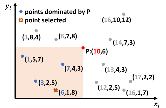
Now we describe the CoveredBy function. We will implement it using the Range function introduced in Appendix C. We present the pseudocode in Alg. 7. The function CoveredBy ( $B_{\mathit{in}},\mathcal{V}$ ) finds a batch of sorted elements $B_{\mathit{out}}\subseteq\mathcal{V}$ , which are covered by a batch of sorted points $B_{\mathit{in}}\subseteq\mathcal{U}$ . Recall that each point $\langle x_{i},y_{i},\mathit{dp}_{i}\rangle$ is a triple. The vEB tree $\mathcal{V}$ is a Mono-vEB tree. The points in $\mathcal{V}$ are keyed on $y_{i}$ . For two points $p_{1}=\langle x_{1},y_{1},\mathit{dp}_{1}\rangle$ and $p_{2}=\langle x_{2},y_{2},\mathit{dp}_{2}\rangle$ , we say $p_{1}$ covers $p_{2}$ if $y_{1}<y_{2}$ and $\mathit{dp}_{1}\geq\mathit{dp}_{2}$ . The Mono-vEB tree maintains a set of points that do not cover each other. In other words, with increasing $y$ values, their $\mathit{dp}$ values must also be increasing.

To find all points covered by the points in $B_{\mathit{in}}$ , we first observe that each point in $B_{\mathit{in}}$ covers a set of consecutive points in $\mathcal{V}$ . Take the $i$ -th element $B_{\mathit{in}}[i]$ as an example, it covers all points in $\mathcal{V}$ such that they have keys ( $y$ coordinates) larger than $B_{\mathit{in}}[i].y$ , but have $\mathit{dp}$ values smaller than or equal to $B_{\mathit{in}}[i].\mathit{dp}$ . Since $\mathit{dp}$ values in $\mathcal{V}$ are monotonically increasing with the key ( $y$ coordinates), such points covered by $B_{\mathit{in}}[i]$ must be a range of points. Such range (if any) starts with the successor $s$ of $B_{\mathit{in}}[i].y$ (if the $\mathit{dp}$ value of $s$ is no larger than $B_{\mathit{in}}[i].\mathit{dp}$ ). Also, for any point in $\mathcal{V}$ that is covered by more than one points in $B_{\mathit{in}}$ , we only need to consider it once. Therefore, when finding the points covered by $B_{\mathit{in}}[i]$ , we can just consider the range from $B_{\mathit{in}}[i]$ to $B_{\mathit{in}}[i+1]$ . More precisely, we should consider range $[s,e]$ , where $s=\textsc{Succ}(\mathcal{V},B_{\mathit{in}}[i].y)$ , and $e=\textsc{Pred}(\mathcal{V},B_{\mathit{in}}[i+1].y)$ . For the last point in $B_{\mathit{in}}$ , the upper bound of the range can be set to $U$ . This gives an initial range of points that may be covered by $B_{\mathit{in}}[i]$ . Note that the lower bound $s$ of the range is tight - either the range starts from $s$ (if the $\mathit{dp}$ value of $s$ is no larger than $B_{\mathit{in}}[i].\mathit{dp}$ ), or $B_{\mathit{out}}$ is empty. We only need to find a tight upper bound $e^{\prime}\leq e$ , such that $e^{\prime}$ is the last point in $\mathcal{V}$ that is covered by $B_{\mathit{in}}[i]$ .

For each point in $B_{\mathit{in}}[i]$ , the range that it is responsible for searching is independent with other ranges. Therefore, we can deal with all such ranges in parallel. For $B_{\mathit{in}}[i]$ , we first use function FindIndex to find the tight upper bound $e^{\prime}$ , which is the last point with $\mathit{dp}$ value smaller than $B_{\mathit{in}}[i].\mathit{dp}$ . In particular, FindIndex $(\mathcal{V},\mathit{dp}^{*},s,e)$ means to search the key range $[s,e]$ in Mono-vEB tree $\mathcal{V}$ , and report the last point in this range with $\mathit{dp}$ value no larger then $\mathit{dp}^{*}$ . Note that the $\mathit{dp}$ values in the Mono-vEB tree $\mathcal{V}$ is monotonically increasing, we can use an binary-search-based algorithm to find $e^{\prime}$ . Instead of directly starting a binary search, this function will first repeatedly apply Succ on the starting point $s$ for $\log U$ times. We do this to guarantee work-efficiency of the algorithm (see discussions later). We stop this process of applying Succ to $s$ when a point with $\mathit{dp}$ value larger than $\mathit{dp}^{*}$ is found, and the previous point must be the last point with $\mathit{dp}$ value smaller than $\mathit{dp}^{*}$ . Another possible case is that when we call Succ, we reach the upper bound $e$ . In this case, $e$ is the last point with $\mathit{dp}$ value smaller than $\mathit{dp}^{*}$ , and we can return $e$ . If after chasing Succ for $\log U$ times, the $\mathit{dp}$ value of $s$ is still smaller than $\mathit{dp}^{*}$ , we can start a regular binary search to find $e^{\prime}$ , which is presented as function BinarySearch. Finally, the function FindInterval will give the tight upper bound of the range of points covered by $B_{\mathit{in}}[i]$ . We will store this return value as $e^{\prime}$ (Alg. 7).

Finally, to get the list of points covered by $B_{\mathit{in}}[i]$ , we can directly use the upper- and lower-bounds $s$ and $e^{\prime}$ , and call the Range function to collect them in list $D[i]$ . The final result will be obtained by combine all such lists $D[1..|B_{\mathit{in}}|]$ . Fig. 11 present an example of the CoveredBy function.

We now analyze the cost of CoveredBy.

Theorem D.1.

The CoveredBy $(B_{\mathit{in}},\mathcal{V})$ function has $O(m\log\log U)$ work and $O(\log U\log\log U)$ span, where $U$ is the universe size of the vEB tree $\mathcal{V}$ , and $m$ is the total size of the input and output batch $|B_{\mathit{in}}|+|B_{\mathit{out}}|$ , i.e., the total number of points in the input $B_{\mathit{in}}$ and those covered by any point in $B_{\mathit{in}}$ .

Proof.

We start with the analysis of the work. We will show that, when processing $B_{\mathit{in}}[i]$ , the work of the FindIndex function and the corresponding Range function is $O((1+m^{\prime})\log\log U)$ , where $m^{\prime}=|D[i]|$ is number of points returned by the Range function.

From Thm. C.1, we know that Range has $O(m^{\prime}\log\log U)$ work, so we will focus on analyzing the work of FindIndex. We analyze two cases.

•

$m^{\prime}\leq\log U$ . In this case, FindIndex will return from Alg. 7 or Alg. 7. In this case, we have called Succ $m^{\prime}$ times, and the total work is $O(m^{\prime}\log\log U)$ .
•

$m^{\prime}>\log U$ . In this case, FindIndex will first call Succ for $\log U<m^{\prime}$ times, and the total work is $O(\log U\log\log U)=O(m^{\prime}\log\log U)$ . The algorithm then performs a binary search. Note that each step in BinarySearch needs to call Succ and Pred, costing $O(\log\log U)$ work. In total, the BinarySearch function takes $O(\log U\log\log U)=O(m^{\prime}\log\log U)$ work.

The work for calling Pred and Succ is also $O(\log\log U)$ . In summary, the work of one FindInterval has work $O((1+m^{\prime})\log\log U)$ for output size $m^{\prime}$ . Adding all the $|B_{\mathit{in}}|$ loop rounds together, the total work is $O((|B_{\mathit{in}}|+|B_{\mathit{out}}|)\log\log U)$ .

We then analyze the span. The longest dependence chain appears in either the $O(\log U)$ invocations to Succ (the sequential for-loop on Alg. 7), or the BinarySearch ( $\log U$ steps, each calling Succ and Pred). Both of them and Range have span $O(\log U\log\log U)$ . Therefore, the span of the algorithm is $O(\log U\log\log U)$ . ∎

Appendix E Making Range-vEB Space-Efficient

The space bound for a plain vEB tree is $O(U)$ . For a Range-vEB tree, since the universe size for each inner vEB tree is $O(U)=O(n)$ and $n$ inner trees in total, the total size will be $O(n^{2})$ . This is space-inefficient and even initialize the tree may make the WLIS algorithm itself work-inefficient. However, note that the total number of possible elements in Range-vEB is at most $O(n\log n)$ , the same as a regular range tree. In this section, we discuss solutions to make our Range-vEB space-efficient.

Many approaches can make a vEB tree space-efficient sequentially, i.e., using $O(n)$ space when there are $n$ keys present in the tree. One of the approaches is to store the cluster arrays using a size-varying hash table instead of an array. As such, the total space consumption will be proportional to the number of existing keys in the vEB tree. However, this makes our algorithms and bounds randomized, and also complicates our parallel algorithms.

Here we propose a solution based on relabeling all keys in each inner tree. In particular, we will make the outer tree a perfectly balanced tree, and its shape and organization are fixed and never change during the algorithm. Once we build the outer tree of the Range-vEB tree, we know exactly which keys should present in each of the inner tree, and thus its size upper bound. For a specific tree node $\tau$ in the outer tree with subtree size $n^{*}$ , its inner tree size is at most $n^{*}$ . Let $S$ be the set of the $n^{*}$ points in $\tau$ ’s subtree. Note that unlike a range tree, where the inner tree of $\tau$ is an index on the entire set $S$ , the inner tree in Range-vEB tree is a Mono-vEB tree. It maintains the staircase of $S$ , which can only be a subset of $S$ . In this case, we will relabel the keys in $S$ to be $0$ to $n^{*}-1$ , and the existing keys in the inner tree. To do this, we have to preprocess all points, and build the outer tree in the Range-vEB tree first. Then for each point (each object in the input sequence $A$ ), we find all the $O(\log n)$ inner trees it appears in. In turn, this gives the set of points for each inner tree, and we relabel each of them. Based on the results, we will maintain $O(\log n)$ lookup tables for each input object, which is the new label in each of the inner tree containing it. For each of the inner tree, we also maintain a lookup table that maps a label to the original input object. In all the algorithms described on the inner trees of Range-vEB tree, we use the new labels as the key, instead of the original key in universe $O(n)$ .

For an inner tree at level $l$ (the root is at level $0$ ), the universe of the inner tree is $O(n/2^{l})$ , i.e., at most $O(n/2^{l})$ points are included in this inner tree. Therefore, the total size of the inner trees is $O(n\log n)$ .


(a). LIS. $\bm{n=10^{8}}$ .	(b). LIS. $\bm{n=10^{9}}$ .	(c). LIS. $\bm{n=10^{9}}$ .	(d). Weighted LIS. $\bm{n=10^{8}}$ .
Line pattern.	Line pattern.	Range pattern.	Line Pattern.

Parallel Longest Increasing Subsequence and van Emde Boas Trees

Abstract.

1. Introduction

Theorem 1.1 (LIS).

Theorem 1.2 (WLIS).

Theorem 1.3 (Parallel vEB Tree).

2. Preliminaries

3. Longest Increasing Subsequence

Definition 3.0 (Prefix-min Objects).

Lemma 3.0.

Theorem 3.3.

Theorem 3.4.

Proof.

4. Weighted Longest Increasing Subsequence

4.1. Parallel WLIS based on Range Tree

Theorem 4.1.

4.2. WLIS Using the Range-vEB Tree

Proof of Thm. 1.2.

5. Parallel van Emde Boas Trees

5.1. Review of the Sequential vEB Tree

5.2. Our New Results

5.2.1. Batch Insertion.

Theorem 5.1.

Proof.

5.2.2. Batch Deletion.

Definition 5.0 (Survivor Mapping).

Theorem 5.3.

5.2.3. Range Query.

6. Experiments

7. Related Work

8. Conclusion

Acknowledgement

References

Appendix A Output the LIS from Algorithm 1

Lemma A.0.

Proof.

Lemma A.0.

Proof.

Appendix B Additional Proofs

B.1. Proof of Lemma 3.2

Proof.

B.2. Solving the Recurrences in Thm. 5.1

Lemma B.0.

Proof.

Lemma B.0.

Proof.

B.3. Proof of Thm. 5.3

Proof of Thm. 5.3.

Appendix C Range Query for vEB Trees

Theorem C.1.

Proof.

Appendix D The CoveredBy Function for Range-vEB Trees

Theorem D.1.

Proof.

Appendix E Making Range-vEB Space-Efficient

Parallel Longest Increasing Subsequence and
van Emde Boas Trees