PANTS: Practical Adversarial Network Traffic Samples
against ML-powered Networking Classifiers
Abstract
Multiple network management tasks, from resource allocation to intrusion detection, rely on some form of ML-based network-traffic classification (MNC). Despite their potential, MNCs are vulnerable to adversarial inputs, which can lead to outages, poor decision-making, and security violations, among other issues.
The goal of this paper is to help network operators assess and enhance the robustness of their MNC against adversarial inputs. The most critical step for this is generating inputs that can fool the MNC while being realizable under various threat models. Compared to other ML models, finding adversarial inputs against MNCs is more challenging due to the existence of non-differentiable components e.g., traffic engineering and the need to constrain inputs to preserve semantics and ensure reliability. These factors prevent the direct use of well-established gradient-based methods developed in adversarial ML (AML).
To address these challenges, we introduce PANTS, a practical white-box framework that uniquely integrates AML techniques with Satisfiability Modulo Theories (SMT) solvers to generate adversarial inputs for MNCs. We also embed PANTS into an iterative adversarial training process that enhances the robustness of MNCs against adversarial inputs. PANTS is 70% and 2x more likely in median to find adversarial inputs against target MNCs compared to two state-of-the-art baselines, namely Amoeba and BAP. Integrating PANTS into the adversarial training process enhances the robustness of the target MNCs by 52.7% without sacrificing their accuracy. Critically, these PANTS-robustified MNCs are more robust than their vanilla counterparts against distinct attack-generation methodologies.
1 Introduction
Managing networks involves tasks such as performance routing, load balancing, and intrusion detection and is extremely challenging due to the highly-diverse, heavy-tailed, and unpredictable inputs, i.e., network traffic. ML-based network-traffic classification (MNCs) provides a compelling alternative for handling these complex tasks more efficiently [18, 33, 11, 32, 23, 10, 20, 19, 43]. However, like other ML-based solutions [35, 15], MNCs are vulnerable to adversarial inputs, that is, inputs meticiously perturbed to deceive the MNC. Attackers can exploit this to compromise critical network infrastructure by subtly perturbing traffic characteristics like packet sizes and inter-arrival times, leading to security breaches or downtime. Beyond being dangerous, these attacks are particularly practical in the networking domain, where multiple entities have access to network traffic.
What is critically lacking is a systematic framework for network operators and MNC designers to enhance the robustness of MNCs against attackers. This involves identifying adversarial inputs, meaning perturbations on original packet sequences that deceive the target MNC into misclassifying them. Operators can then use these inputs to: (i) refine and optimize the MNC by exploring different models, architectures, or features; (ii) assess the attack surface of their MNCs, understand the potential consequences and plan accordingly; and (iii) use them to strengthen MNCs against realistic threat models through re-training or fine-tuning. Critically, operators will not use or take the framework seriously if the generated adversarial inputs are (i) not realizable, meaning they do not fall within a realistic attacker’s capabilities, or (ii) do not retain the semantics of the original sequence, meaning the ground-truth label of the perturbed inputs has changed. In fact, we show that realizable and semantics-preserving adversarial inputs are more useful for adversarial training compared to purely adversarial ones.
While there are numerous tools for generating adversarial samples in the Adversarial Machine Learning (AML) literature [16, 27, 7] they are not directly applicable to MNCs. First, AML tools are built for systems that are end-to-end differentiable, which makes them unsuitable for typical MNCs that include a feature engineering module to transform packet sequences into feature vectors before they are fed to the ML model. Although AML tools can generate adversarial feature vectors, there is no guarantee these vectors can be reverse-engineered into valid packet sequences. Even if a valid packet sequence exists, the perturbations needed to convert the original sequence into an adversarial one may exceed what a realistic attacker could achieve. Second, it is uncertain whether AML-generated samples are preserving the semantics of the original packet sequence while deceiving the MNC. Although AML techniques often incorporate a perturbation budget (expressed as a norm), this concept does not translate well to networking traffic. For example, perturbing a VoIP flow (packet sequence) to resemble web browsing by delaying packets might deceive a traffic classifier but degrades the original flow’s performance, making the call unusable. Critically, adversarially training an MNC with non-realizable or non-semantics-preserving samples (i.e., directly using what AML generates) will degrade the MNC’s accuracy without significantly improving robustness as we show in §2.
Learning-based approaches such as Amoeba [26] use reinforcement learning to directly generate adversarial traffic sequences. Being black-box approaches, such tools are great for attackers to fool ML-powered applications. However, the lack of diversity in adversarial samples, their instability, and training hardness make them less effective for assessing and enhancing the robustness of MNCs from the network operator’s perspective, as we show in our evaluation.
To address these shortcomings, this paper presents PANTS, a framework to generate Practical Adversarial Network Traffic Samples that are realizable for various threat models and semantic-preserving. PANTS integrates traditional methods for generating adversarial samples (AML), such as Projected Gradient Descent (PGD) [27] or Zeroth-order Optimization (ZOO) [7], with formal methods, concretely a Satisfiability Modulo Theories (SMT) solver. The AML perturbs the original inputs (packet sequences or features) in a manner that maximizes their distance (e.g., loss for MLP) from the original decision boundaries with consistently high success rate. The SMT solver finds packet sequences that do not diverge too much from the AML’s output but are realizable, and consistent with the threat model and preserve the semantics of the original packet sequence. To achieve this, we encode the feature engineering, the threat model, and other networking constraints needed for semantic preservation into logical formulas. Among other optimizations, PANTS iteratively adds and removes constraints that come from the AML, prioritizing those that have a substantial effect on confusing the classifier. Finally, we integrate PANTS into an interactive training process that enhances the target MNC.
We have evaluated PANTS against three distinct ML-powered network classifiers, each implemented with different models and processing pipelines. PANTS finds adversarial, realizable and semantic-preserving samples with 35.31% success rate in median, that is 70% and 2x higher than two SOTA methods. Despite being a white-box approach, PANTS works well with gradient (e.g., transformer encoder) and non-gradient (e.g., random forest) models and various processing pipelines, including those containing non-differentiable components (e.g., feature engineering). Importantly, we integrate PANTS into a novel adversarial training pipeline, which improves MNCs’s robustness against both PANTS-generated inputs and Amoeba-generated inputs. We will, of course, make PANTS and our use cases publicly available to facilitate further research and to improve reliance on MNCs.
Ethics Statement: This work doesn’t raise any ethical issues.
2 Motivation & Limitations of Existing Work


To highlight the need for a framework that generates adversarial inputs to help operators assess and mitigate the vulnerabilities of their MNCs, we present a specific use case: an ML-based classifier that exposes the network to a range of exploits, from giving attackers an unfair advantage to causing outages, regardless of the exact implementation of the MNC. We then outline the essential properties required for such a framework and explain why existing solutions are insufficient.
2.1 Motivating use case
Consider a network operator that uses an ML-based traffic classifier to distinguish real-time applications (e.g., online gaming). The operator uses this information to optimize routing: real-time applications use fast but low-bandwidth network paths. This is one of the multiple network management tasks for which network operators could use a ML-based traffic classifier (built with Multilayer Perceptron-MLP, Random Forest, Transformers [25, 6, 18, 33, 11]) and benefit from its ability to learn complex patterns directly from data. While highly useful, this MNC exposes the network to various exploits. Two representative examples include attackers controlling (i) the end hosts of the communication or (ii) an in-network component. In the former case, a malicious (or simply “rational”) application developer could manipulate the traffic generated by her application to be misclassified as gaming by the network’s MNC, hence gaining an unfair performance advantage over competitors. This could be achieved by subtly altering the size of some packets or delaying specific packets without significantly impacting the overall performance of her application’s traffic. In the latter case, a malicious or compromised router in-path can increase the volume of traffic routed through the fast but low-bandwidth path by subtly altering the non-real-time traffic to cause the MNC to misclassify it as real-time. These perturbations would result in congestion in the low-bandwidth path, leading to delays or even downtime for actual real-time traffic, which is vital for the network’s profitability. The attacker cannot inject packets because that would be detectable from the application perspective, but she can delay packets.
ML network classifiers are vulnerable to adversarial inputs. Fig. 1 illustrates the likelihood of an attacker controlling end hosts (e.g., a malicious app developer) to successfully manipulate their traffic to cause an MNC to misclassify it (predict a favorable for the attacker label). The results show that, despite the high accuracy of the models during testing, the attacker can deceive classifiers implemented with MLP, CNN, and a transformer with success rates of 81.12%, 94.25% and 99.80%, respectively. While we identified these manipulations (adversarial inputs), hence the vulnerability of the MNCs using PANTS, which is a white-box approach with complete access to the MNC’s implementation, this does not diminish the significance of the risk they pose. Security through obscurity is never a sound strategy, and network operators should be prepared for (or at least aware of) the worst-case scenario where an attacker has complete knowledge of their system.
Adversarial training trades accuracy for vulnerability. Fig. 1 also shows the trade-off between inaccuracy and vulnerability in MNCs. Indeed, an operator could leverage authentic (off-the-shelf) adversarial training to shield an MNC against adversarial inputs. However, by doing so, she will sacrifice the accuracy of the MNC, meaning the baseline performance of the MNC in more common inputs will degrade. By authentic adversarial training, we refer to training a robustified model with the help of PGD [27]. During model training, the original training samples are substituted with their PGD-generated adversarial counterparts in each training iteration.
2.2 Requirements
Next, we elaborate on the requirements of a framework that generates adversarial samples and use them to enhance the robustness of MNCs before we explain why existing approaches fall short.
Adversariness & Semantic preservation . The framework needs to generate inputs that are adversarial, meaning that they are capable of misleading MNCs into producing an incorrect classification. To ensure that the classification is indeed incorrect, these inputs should be created by meticulously applying perturbations to the original labeled samples without altering their semantics. In other words, each adversarial input should still represent the same underlying meaning or class as the original, which is described as a set of constraints on the adversarial input. The closest notion of semantics in the image domain is the perturbation budget, which sets a maximum allowable distance between the original and perturbed image [27]. However, such a metric doesn’t translate directly to the networking domain, where there are dependencies across packets or features of each input, which perturbations should respect. We assume that semantics can be expressed as constraints on the variables of the input (not only as a distance between the adversarial and the original), and the framework should provide the means to respect them
Realizability. The framework should provide mechanisms to constrain the generated adversarial inputs according to domain-specific rules and a configurable threat model, which the operator will consider reasonable. Concretely, adversarial samples must represent valid packet sequences — for example, TCP should never acknowledge a packet before it is sent. Further, each adversarial input must be created by applying perturbations that are within the capabilities of the threat model to an original input. Optimizing the model by training it on unrealizable inputs that it will never encounter is not only wasteful but can also degrade its performance on common inputs, as we show in §4.5. For instance, an in-network attacker cannot alter an encrypted packet in a way that evades detection, so examining such scenarios would be unproductive.
Generality. The framework needs to be able to work in various classification pipelines. Unlike the image domain, where end-to-end neural network-based (NN-based) models play a dominant role in various tasks, networking applications employ a wide spectrum of classification models and pipelines. Concretely, the framework needs to work for typical MNCs, which include non-differentiable and non-invertible feature engineering modules to extract statistical features from the given packet sequence, followed by a differentiable or non-differentiable ML model such as Multi-layer perception (MLP) or Random Forest (RF) for classification. The framework should also work for MNCs that directly encode the packet sequence into a sequence of packet length, packet direction, and inter-arrival times only. In the latter case, the encoded sequence is fed into deep learning models such as Transformer (TF) or convolutional neural network (CNN) for classification.
2.3 Limitations of existing work
Having described the requirements of a framework that aims to help network operators, we explain why various lines of work that generate synthetic or adversarial networking inputs fail to satisfy them. We elaborate on works that generate adversarial images (i.e., AML) in §3.2.
Synthetic data generation Networking-specific generative models such as NetShare [44] and Netdiffusion [21] have shown strong promise in generating high-fidelity synthetic traffic. While synthetic traces can, in some cases, be used to improve the performance of ML models [22], the synthetic traces are unlikely to mislead an ML classifier, and even if they do, one has no way of knowing the correct label.
Black-box RL-based techniques While useful for aspiring attackers, black-box RL-based approaches [14] for generating adversarial examples against MNCs are incapable of meeting our requirements. Amoeba [26], for example, trains an agent to perturb each packet to maximize the likelihood that the altered flow will deceive the MNC. Amoeba fulfills the generality requirement as it is black-box, and can fulfill realizability if trained with the right actions. Still, Amoeba’s outputs are not always semantic-preserving and adversarial because there is no way to guarantee those during inference. Also, as we show in our evaluation, Amoeba’s generated adversarial inputs are less effective in robustifying MNCs during adversarial training, possibly because it (over)exploits a vulnerability rather than trying to find new ones. This is a reasonable strategy for an attacker, which is the focus of such a black-box approach.
White-box gradient-based techniques Among the group of white-box and gradient-based approaches (which includes AML that we discuss in §3.3), a representative example (due to the focus on networking inputs) is BAP [29]. BAP adversarially trains a generator to create perturbation (e.g., delay, number of added dummy bytes) on every single packet of a packet sequence such that the distance (e.g., loss) between the predicted label of the perturbed sequence and its ground truth is maximized. Because BAP uses gradient for maximizing the loss it does not work for non-end-to-end differentiable MNCs, hence failing the generality requirement. Further, by perturbating each packet independently, we cannot enforce semantics, which can be flow-wide. We compare against BAP in §5.
Robustness certification Ideally, network operators would resort to robustness certification [24, 39, 41, 36, 42] to understand the vulnerability of their MNCs. Applying such techniques in networking is not trivial, BARS [38], for instance, considers the robustness guarantee for perturbations at the feature level instead of the guarantee at the packet level and hence cannot incorporate threat models. Indeed, a small perturbation in the flow, such as injecting a dummy packet in a small interarrival time, can easily exceed its robustness region in the feature space. More importantly, though, certified robustness cannot match the empirical robustness using adversarial training [40, 28], which is, in fact, more indicative of the real risk.
3 Overview
Our goal is to build a framework that generates adversarial samples that can be used to assess and improve the robustness of an MNC while fulfilling the requirements in §2.2. After we formulate our problem, we elaborate on the opportunities and challenges of traditional AML in solving it. Finally, we explain the insights that drove our design.

3.1 Problem formulation
Consider an ML model used to implement a network classifier where represents the set of possible labels. We define as the input to . This can be the result of a feature engineering function, denoted as on a sequence of packets p= from the set where each is a packet arrived at time or a subset of the sequence of packets p. Each packet can be represented by various attributes, including its size flags, direction etc. We assume that for every MNC, the following dataset exists. Let be the dataset, where are the feature vectors obtained by applying to raw network data and are the corresponding label.111Applying directly on a truncated packet sequence is possible and a simplification of the problem we describe.
We define a threat model as a set of pertubations, () on the original packet sequences, , to generate adversarial packet sequences , (). is adversarial if , meaning that the perturbed flow will be misclassified by and preserves the semantics of . Semantics are flow-level constraints on i.e., constraints that can be dependent on the whole packet sequence not just each packet indecently.
Our goal is to design a framework that generates packet sequences from such that are adversarial to , semantic-preserving to , and are within the capabilities of a threat model.

3.2 The promise of Adversarial ML
At first glance, adversarial ML (AML) seems to be the right approach for our problem definition and requirements. First, AML generates adversarial inputs against ML-based systems, typically in the image domain. Concretely, given a trained ML classifier with model parameters , an original image sample with its ground truth label , PGD perturbs to be an adversarial sample by iteratively running , . is the target loss function, measuring the distance of the predicted label of and , and represents the capability of attack, which is usually defined as -ball distance around . The perturbation starts from the original sample . In each iteration, the sample is moved by following the direction of the gradient of . After modification, the intermediate value is projected to be within the attack capability by clipping it to a predefined -ball distance around . In each iteration, we expect to have higher possibility to be misclassified. Second, AML is quite general, despite using gradient. In fact, there are AML methods that do not rely on a gradient or whose gradient information is inaccessible to the attacker, such as ZOO [7]. ZOO uses a combination of techniques, such as coordinate descent and importance sampling, to estimate the gradient for getting adversarial samples. Although it was initially designed for black-box attacks against NN-based models, it can be extended to attack other models such as Random Forest and XGBoost [5, 1, 2].

3.3 AML limitations
While AML can generate an adversarial sample and generalize at least across some models, AML does not provide realizability and semantics preservation. At a high level, the root cause of the problem is that AML finds adversarial inputs using backward reasoning (i.e., targets a change in the predicted label), but semantics preservation and realizability require forward reasoning, i.e., are defined on the input [9, 13]. In the image domain, this is not a problem as classifiers are end-to-end differentiable: images are directly fed into the ML model for classification, which is typically neural network-based. AML modifies input pixels directly and independently from each other (as they do not need to adhere to any rules beyond being in a range) to increase the loss informed by the gradient. Such techniques also include a budget to constrain just the pixel-to-pixel distance from the original with no other obligation.
However, in the networking domain, the traffic is often processed by the feature engineering module, which generates feature vectors that are fed to the ML model. While gradient information can still guide the modification of each feature to increase loss, it is unclear how to map modifications to the feature vector into the corresponding packet sequence as the feature engineering is non-differential and non-invertible. In fact, there is no guarantee that a perturbed feature vector would have a corresponding valid packet sequence as AML changes each feature independently, making contradicting decisions. For example, suppose an ML-powered intrusion detection system whose feature set includes both minimum and maximum packet inter-arrival times (, ). Since AML does not understand the two features are dependent, in other words, that must always hold, it is possible for AML to decrease the value of and increase such that . In this case, while the generated feature vector might be adversarial in that it might be misclassified by the intrusion detection system, it is not a realizable sample i.e., there is no packet sequence that would ever result in this feature set. In short, using the perturbed feature vectors is like defending against an impossible attack. While one can try to use a mask [30] to only allow AML to change a subset of the features that are not dependent, that would reduce the inputs that AML can find. Indeed, while AML can run with as few as a single feature there is no guarantee that the generated sample would be adversarial.
Even if the target model does not use (non-differentiable) feature engineering or if one somehow finds a packet sequence that is consistent with the AML adversarial feature vector, the packet sequence might still fall outside the capabilities of the threat model, violate any network constraints, or break the semantics of the original flow. For example, suppose the threat model only allows injecting packets, and flow duration and packets per second are two features extracted by the feature engineering module. The number of packets can be derived from . If derived from the adversarial features is less than the number of packets in the original flow, even though one can find an adversarial packet sequence consistent with the adversarial features, it still falls outside the capabilities of the threat model. Similarly, for a deep NN that is directly accepting the packet sequence as input, the AML-generated adversarial sequence could change the interarrivals in a way that is impossible for any congestion control algorithm or in a way that makes the connection unusable because it is too slow in the beginning.
3.4 PANTS: AML for networking
To address the inherent challenges in applying AML to MNCs, we integrate a formal-method component to ensure the realizability and semantics-preservation of the produced adversarial samples. Our first insight is to use logical formulas to model the feature-engineering process that turns packet sequences into feature vectors, and sequence-level constraints for MNCs with no feature-engineering, effectively encoding input dependencies. Further, we encode threat-model capabilities, networking rules and semantics into flow-wide or packet-level constraints and ask an SMT (Satisfiability Modulo Theories) solver to find a packet sequence that satisfies them. If the answer is “UNSAT”, the adversarial features are not realizable under the given threat model, semantic, and networking constraints. Observe that SMT supports both forward and backward reasoning, hence can connect the requirements for adversariness with realizability and semantics. Critically, this makes PANTS extendible to any definition of semantics.
As feature engineering modules, and sematics definition can be arbitrarily convoluted, a naive serial combination of AML with SMT will also fail because most of the AML-generated samples would not have a corresponding packet sequence that is realizable. Our second insight to address this challenge is that not all AML-generated features need to be honored for the sample to be adversarial. We design an optimization loop containing an AML component (e.g., PGD or ZOO), an SMT solver, and the target MNC, which iteratively checks whether a subset of the AML-produced adversarial features (or perturbations) can result in a realizable packet sequence until enough adversarial and realizable samples are collected. Instead of trying every possible subset of features, our third insight is to identify the most vulnerable adversarial features i.e., those that are both easy to tweak based on the threat model and important enough for the target ML model to affect its output. Critically, though, PANTS might opt out of constraints that make the generated samples adversarial but not constraints that make samples realizable or semantics preserving, which are always satisfied.
4 Design
4.1 PANTS end-to-end view
We provide an end-to-end view of how PANTS generates adversarial packet sequences, shown in figure 4. The procedure includes 8 steps, starting from feeding in the original packet sequence to getting the adversarial and realizable packet sequence returned by PANTS.
Step ①: Given an original packet sequence, we use the feature engineering module in the target application to extract its features. Step ②: After getting the features, PANTS uses the canonical AML methods (PGD, ZOO) to generate an adversarial feature vector (sample). The generation process interacts with the ML classifier to ensure the adversariness of the generated sample. Note that the generated adversarial features are not strictly required to be within a predefined -ball distance around the original features since the capability of the attacker (threat models) for the networking applications is different from the image domain described in §3.2. Step ③: Given the generated adversarial feature, PANTS runs an iterative process to find (multiple) adversarial and realizable packet sequences using a feature selector and an SMT solver. The feature selector first determines the importance of each feature in keeping the generated features adversarial. Step ④: The feature selector begins to construct a selected feature list by considering one new feature each time, starting by appending the most important feature and proceeding in descending importance order. Step ⑤: Given the selected features, we encode these features’ dependencies, threat model constraints, and networking constraints into formulas and query the SMT solver to find a packet sequence to satisfy them. Step ⑥: If the SMT solver returns “UNSAT”, i.e., it cannot find a packet sequence, the feature selector pops out the latest appended feature from the selected feature list. The iterative process continues to step ④ to append the next most important feature and repeat step ⑤ and ⑥ until the first most important features are considered. Step ⑦: The packet sequence(s) found by the SMT solver are guaranteed to be realizable since the threat models are encoded into the satisfiable formulas. Finally, we need to confirm the adversariness of these realizable packet sequences. We feed these packet sequences into the feature engineering module again to get the corresponding feature vectors. Step ⑧: We feed these feature vectors into the ML classifier to get the predicted label. We compare the prediction result with the ground truth label of the original packet sequence. If they are different, the realizable packet sequences found by the SMT solver are adversarial, and the feature vectors correspond to realizable packet sequences. Note that these packet sequences are very likely to be adversarial, given that the feature selector prioritizes the use of the most important features.
4.2 SMT formulations
We leverage an SMT solver to help find adversarial packet sequences. We encode into formulas the feature dependencies, the threat model constraints, the networking and the semantics constraints. The SMT solver determines whether the resulting formulas are satisfiable.
We illustrate with an example. Assume an original network flow that only has three packets, p= where . represents the direction of the packet, where means packets sending from the connection initiator to the receiver (forward packet) and vice versa. and represent the inter-arrival time and packet length for each packet . Adversarial features dictate that the average inter-arrival times should be , the maximum inter-arrival times should be and the average packet length is . The threat model only allows to delay forward packets and append dummy payload to the forward packets. To preserve the semantics meaning, the accumulative delay cannot exceed 20% of the original duration. We thereby define four variables , , and . They are representing the delay and the appended payload for and . The perturbed flow p’ can be formulated as p’. Then, the formula for the SMT solver is
| (1) | |||
| (2) | |||
| (3) | |||
| (4) | |||
| (5) | |||
| (6) | |||
| (7) |
Equation (1), (2), (3) and (4) are forcing the adversarial packet sequences found to be consistent with the average (equation (1)), maximum (equation (2) and (3)) inter-arrival times and the average of packet length (equation (4)) in the adversarial features, maintaining the feature dependency. Equation (5) ensure that the packet sequence is complied with the threat model that it can only delay and append dummy payload to the forward packets. Equation (6) and (7) formulate the network and semantics constraints.
4.3 Adversarial packet sequence identification
Feature importance determination.
Considering all features will be too computationally expensive for the SMT solver and can lead to unsatisfiable combinations. Thankfully, not all features are equally important in keeping the packet sequences adversarial. Thus, we design a feature importance ranking algorithm and generate packet sequences that are only consistent with the most important features. Since AML methods are designed to perturb features to maximize the chance that they will be misclassified, our intuition is that the features that have been changed the most play a more important role in adversariness. Thus, after normalizing all the features into the same scale, the importance of each feature is determined by the difference in that feature value between the adversarial and the original one.
As an example, suppose there is a VPN flow p, and its extracted features are min and max of interarrival times, i.e., [, ]. AML generates adversarial features to be and so that it is classified as Non-VPN. Unfortunately, SMT cannot find solutions consistent with these two features. Therefore, we want to select the most important feature and find the packet sequences that only comply with that one. Assume that is more important than . Then, the SMT solver finds solutions only for . After that, we construct the packet sequences using these solutions and recalculate the maximum interarrival times of the given packet sequences . Since is consistent with AML’s decision and is the most important feature, we expect that the new features [, ] will still be adversarial.
Find adversarial and realizable packet sequences using iterative testing. After determining the important features, the next questions are: (i) how many important features are necessary so that the conforming packet sequences are adversarial; and (ii) how to ensure that the SMT solver can find packet sequences consistent with these selected important features? To address them, we employ iterative testing, which searches for successful adversarial packet sequence generation, starting with the most important features. Starting with an empty feature list, we iteratively test whether adding the formulas of the next most important (not already explored) feature results in a conforming packet sequence output from the SMT solver. If it does, is appended to the selected features list. Otherwise, the feature is not selected. By adding more and more features, the found packet sequences are more likely to be adversarial. In practice, it is possible that after appending , the solution provided by the SMT solver is already adversarial. However, in order to cover a wider spectrum of adversarial features and enable robustification of the model, the algorithm collects this solution and continues appending for another potential solution until reaches . is a parameter defined by the users, representing the most important features that need to be included in the iterative testing. Setting a small value forces the algorithm to include only a few features, which can hurt the adversariness. Setting it too large results in including too many non-important features, making the generation speed slow without much adversariness improvement. The algorithm details are depicted in alg 1.
4.4 PANTS’ SMT optimizations
The SMT solver’s efficiency in finding adversarial packet sequences is a critical factor for PANTS’ usability. Unfortunately, the SMT solver is often unable to find adversarial packet sequences within a reasonable time frame. The problem is that SMT solvers have scalability limitations and the given formulas can result in very high computational complexity. The complexity depends on many factors, such as the length of the packet sequence, the formulation of capabilities, the number of features to be solved, and the difficulty of solving each feature. We have already discussed restricting the number of used features and prioritizing the evaluation of the most critical features in §4.3. In this section, we focus on optimizing the packet sequence length and the formulation of capabilities.
Network flow chunking and parallelization. A longer packet sequence requires more variables to formulate, which implies a much larger search space for the SMT solver. We address this problem with a combination of a timeout mechanism, network flow chunking, and parallelization.
We first set a time budget for the SMT solver. If the SMT solver cannot find packet sequences within a timeout window, we decrease the computation complexity by dividing a flow into several chunks evenly. The SMT solver is used to find the packet sub-sequences for each chunk. Since each chunk has fewer packets than the whole flow, it is more likely that the SMT solver will be able to find solutions within the timeout limits. After splitting a flow into multiple chunks, some features are difficult to be formulated strictly. For example, when working on a complete flow, it is easy to formulate the maximum packet length feature. After splitting the flow into multiple chunks, the maximum packet length can appear in any chunk. Strictly formulating this feature would require a complicated algorithm, which is in conflict with our motivation to decrease computation complexity and is unnecessary for our use case. To solve this problem, we consider three different types of features. For the first type of features, satisfying their formulas for each sub-sequence will likely result in satisfied formulas for the whole sequence. For example, such features are {max, mean, median, min, std} of {interarrival times, packet length} and number of {packets, bytes} per second. For these features, SMT solves their formulas per chunk. For the second feature type, the accumulation of each chunk’s feature values is equal to that of the whole flow. One typical example is the total duration. For these features, the SMT solver is finding sub-sequences in each chunk consistent with . For other features, such as the number of unique packet lengths, we are not aiming to be consistent with the whole-flow formulas when finding the sub-sequences for each chunk.
Finally, parallel computing can further speed up generation time, since the SMT-solving process for each flow/chunk is designed to be independent.

Inefficient formulation of capabilities can be simplified. Unfortunately, not all the capabilities can be formulated efficiently. The capability to inject packets at any position is one of them. The underlying reason is that multiple dummy packets can be injected at any position. Each combination requires an invocation of the SMT solver. For example, given a flow with four packets, , injecting packet by or can cause different solutions on when asking the packet sequence to comply with the features of backward flow interarrival times. Suppose a threat model that allows injecting at most packets and the packet sequence length is k; formulating this capability into formulas requires SMT to run times to cover all combinations. Therefore, packet injection at any position is very inefficient, and we consider simplifying the formulation to increase the generation speed. Although packet injection at any position requires the SMT solver to find packet sequences multiple times, injecting packets at the end of the flow is efficient since there is only one injection position. Thereby, the SMT solver only needs to run once. We leverage the flow chunking and simplify the implementation of any-position injection by injecting only at the end of each chunk. As we increase the number of chunks, the number of packets per chunk is decreased and the final effect is closer to packet injection at any place.
Figure 5 shows the sample generation speed after the discussed optimizations. PANTS achieves reasonable efficiency by taking less than 1s on generating a single sample in most of the cases. Generally, the generation speed doesn’t show notable difference between threat models, ML models and applications. However, for MLP and RF tested for the in-path threat model, the generation speed varies across different applications. The in-path threat model indicates a limited action space, making SMT harder to find solutions especially for those processing pipelines using feature engineering.
4.5 Adversarial Training with PANTS
Adversarial training is often used to enhance the robustness of ML models. During authentic adversarial training, an AML method (e.g., PGD) replaces each benign sample with an adversarial one for the insufficiently trained version of the model. While useful, this method can hurt the accuracy of an ML model [17, 31] and only applies to NN-based models. To avoid these shortcomings, we adopt an alternative way of adversarial training, in which we augment the training dataset with adversarial samples generated for the sufficiently-trained model to fine-tune it. This methodology is model agnostic, meaning that it can work with any processing pipeline. We also find in §5.2 that this training methodology improves robustness without hurting the model’s accuracy.
5 Evaluation
In this section, we evaluate the efficacy of PANTS in two ways. First, we evaluate PANTS’ capability in generating adversarial realizable, and semantic-preserving flows and compare it with two baselines, Amoeba [26] and BAP [29]. Second, we evaluate the effectiveness of PANTS-generated samples in improving the robustness of the targeted MNCs. We begin by introducing the evaluation setup, and then we discuss some key findings. In summary, PANTS is 70% more likely to find adversarial samples compared to Amoeba in median and 2x more likely compared to BAP. Using PANTS for robustification can have 142% more robustness improvement then using Amoeba without sacrificing the model accuracy.
5.1 Setup
Applications. We select three typical classification tasks to evaluate PANTS. They have diverse objectives, flow statistical patterns, and classification granularity, providing a representative sample of networking applications.
VPN traffic detection is a challenging task for encrypted traffic classification. A well-functioning classifier is trained to determine whether the traffic is VPN. ISCXVPN2016[11] is one of the commonly-used labeled datasets, and includes both VPN and non-VPN traffic. The dataset contains more than million packets grouped into bi-directional flows. Of those, % are non-VPN, and the rest are VPN flows. This is an unbalanced dataset, hence, we include both accuracy and F1 score for more comprehensive evaluation of the model performance.
Application identification (APP) is useful for characterizing mobile traffic from different applications and is crucial for network management tasks such as anomaly detection and resource allocation. UTMobileNetTraffic2021 [18] is a commonly-used dataset that includes mobile traffic from 18 popular applications (e.g., Dropbox, Google Drive, Facebook) under different user activities (e.g., Dropbox-download, Google Drive-upload, Facebook-scroll). It has multiple subsets representing different controlled user activities, such as scrolling the Facebook news feed. We choose one of these subsets that collects application traffic without placing any constraints on user activity. Similar to VPN detection, classification is applied to the bi-directional flows. The selected dataset contains 7,134 bi-directional flows.
Quality of Experience (QoE) inference arises as an important task for all stakeholders, such as ISPs and service providers, due to the rise in the use of Video Conferencing Applications (VCAs). By training various models, multiple QoE metrics can be inferred, e.g., resolution and video bitrate directly from packet traces. The state-of-the-art framework is trained and tested on a dataset called VCAML in a per-second granularity[33]. VCAML contains a large number of single-directional video conferencing flows from Google Meet, Microsoft Teams and Cisco Webex in different resolutions, bitrate, etc. We pick resolution prediction as the task to test our framework. The total number of samples is 37,274, which includes 11 different resolutions, such as 720p, 360p.
The features extracted by the feature engineering module for different applications are listed in the Appendix in §A. All the datasets are applied with basic data cleaning. Any flow with only one packet is removed as calculating interarrival times requires at least two packets.
ML models. For each application, we train four commonly used ML classifiers independently. They are Multilayer Perceptron (MLP), Random Forest (RF), Transformer (TF) and Convolutional Neural-Network (CNN). They exemplify different ML approaches, including (deep) neural network-based and tree-based techniques. Meanwhile, they also represent different processing pipelines. MLP and RF use a non-differentiable and non-invertible feature engineering module, which extracts statistical features that are then used as input to the models to predict the labels. TF and CNN are end-to-end differentiable: packet sequences are directly encoded as a sequence of interarrival times, packet direction and packet length for classification. The maximum sequence length is set to 400. The details of the hyperparameters used for each model are explained in the Appendix in §B. Table 1 shows the performance of these 4 ML classifiers. For each dataset, the training set () and the testing set () are following a 80%:20% random split. ML models are trained on , and the performance is evaluated on .
| Application | Model | Accuracy | F1 Score |
| APP | MLP | 0.7947 | 0.7966 |
| RF | 0.8206 | 0.8202 | |
| TF | 0.7666 | 0.7645 | |
| CNN | 0.7926 | 0.7923 | |
| VPN | MLP | 0.8902 | 0.9437 |
| RF | 0.9400 | 0.9574 | |
| TF | 0.9295 | 0.9287 | |
| CNN | 0.9219 | 0.9214 | |
| QOE | MLP | 0.8070 | 0.8247 |
| RF | 0.8221 | 0.8330 | |
| TF | 0.7819 | 0.7831 | |
| CNN | 0.8203 | 0.8159 |
Attacker’s capability. To show the flexibility of PANTS, we evaluate two realistic threat models. The two models correspond to attackers located at the end host and in-path, respectively. The attackers at the end host are stronger as they can delay packets, inject packets, and append dummy payload to the existing packets. To preserve the flow’s semantics, we consider that the end-host attacker can only delay the flow up to 20% of the original flow’s duration, inject at most 20 packets, and append dummy payload to at most 20% of the packets. Of course any flow-wide or packet-level constraint would work. The in-path attackers are weaker as they can only delay packets. An in-path attacker can only delay at most 20% of the original flow’s duration. Note that our assumption considers a single attacker at a time, thereby restricting the manipulation to one direction of flow. Adding more threat models to PANTS consists of adding the relevant constraints.
Baselines. Since there is no related framework that aims to help the operator assess and enhance the robustness of MNCs, we compare them against the State-Of-The-Art attack generation methods, Amoeba and BAP. Amoeba [26] is an RL-based proposal to attack ML-based censorship. Whilst designed for a different goal, Amoeba also generates adversarial samples against applications that are end-to-end differentiable and that include a non-differential or non-invertible module. Amoeba supports delaying packets, appending dummy payload to the existing packets, and splitting packets into multiple ones. For a fair comparison, we extend Amoeba’s capability to comply with the two evaluated threat models. We also train Amoeba’s agent to respect the flow’s semantics and enforce a budget during inference. We explain the details of our extension in the Appendix in §C.
BAP is to train a generator to create perturbations for each packet. Since BAP [29] does not support applications that include non-differential and non-invertible components, we only consider it for TF and CNN but not MLP and RF. The original implementation of BAP can only support perturbing every packet, so we extend BAP by adding a mask during training and inference to ensure reliability (e.g., only act on forward packets). Although BAP supports per-packet constraints, it does not support flow-wide constraints such as those needed for semantics preservation.
Testbed. Appendix §D details the used CPU/GPU machines.
5.2 Key Findings
Finding 1: PANTS is 70% more likely to find adversarial samples compared to Amoeba in median and 2x more likely compared to BAP.


We first compare PANTS with Amoeba and BAP in their ability to generate adversarial flows for various ML models, applications, and threat models. We run experiments five times and report the Attack Success Rate (ASR), i.e., the ratio of realizable, semantic-preserving and adversarial samples / total original samples for each technique222While PANTS generates multiple adversarial samples per original, for the ASR calculation each original sample can contribute at most one adversarial.. Figure 6 shows the results of ASR. PANTS achieves 35.31% ASR in median while only 19.57% for Amoeba and 10.31% for BAP. Among these three methods, BAP performs the worst in part due to its inability to respect semantics i.e., flow-level constraints.
Compared to Amoeba, PANTS is 51% more likely to find adversarial samples for the end-host threat model in median and 2X more likely for in-path attacks. We observe that Amoeba struggles to find adversarial samples when for an attacker that is in-path. Concretely, for the QoE inference, the ASR for Amoeba is around 0.3% for in-path threat model while PANTS is 37%. PANTS is particularly more effective with the weak threat model compared to Amoeba, showing its more comprehensive nature.
Importantly, PANTS’s ASR is more consistent across runs in all the test cases. This is important as an operator is unlikely to trust the assessment of a tool that reports a different ASR in every run i.e., varying levels of vulnerability for a given MNC. Concretely, the average standard deviation across all the test cases is 0.77 for PANTS, while for Amoeba is 3.12 and BAP is 2.61. For some specific test cases, Amoeba and BAP show ASR with relatively large fluctuations. For example, Amoeba’s ASR on attacking TF ranges from 76.15% to 93.45% and BAP is from 43.89% to 54.25% while PANTS’ ASR only ranges from 99.75% to 100.0% as we observe in Fig. 6(a). The large variance in Amoeba’s results stems from a well-known problem in RL: its inherent instability of training. For PANTS, randomness only comes from the adversarial features generated by PGD and its timeout mechanism. PGD might generate different adversarial features in different runs due to random restarts, which are used in MLP and RF [27]. The time budget in SMT also causes minor randomness by the CPU’s processing speed fluctuation. It turns out that randomness caused by these two factors are small.
Finding 2: Iterative augmentation with adversarial, realizable and semantics-preserving samples improves the robustness of an MNC without hurting its accuracy.
As Amoeba is more general and results in higher ASR compared to BAP, we continue our evaluation on robustification with Amoeba only. Concretely, we robustify the target ML models by iteratively fine-tuning them on a combination of the original dataset with its adversarial counterpart generated by PANTS and Amoeba as the way described in §4.5.
We found that in most of the cases, 3 iterations of robustification are enough when using PANTS to robustify an MNC. The robustified MNC is able to defend the adversarial inputs that are generated by PANTS itself, Amoeba and BAP. For TF in the application APP and QOE under end-host threat model, we train for 5 iterations to reach a desirable ASR. Figure 7 shows a trajectory of ASR when a vanilla MNC is in iterative robustification using PANTS’ samples. During the iterative training the ASR (calculated using PANTS to generate adversarial inputs) drops, meaning that the model is getting more robust. Iteratively training MNCs using adversarial samples generated by Amoeba follows a similar but less dramatic trend. The results are shown in Appendix in the fig. 12.


After robustification, PANTS generates multiple adversarial samples for each benign counterpart in total to cover diverse adversarial samples. Using PANTS, we generate around 1.16-180 samples for each benign sample during robustification based on different threat models, applications and ML models. We also include non-adversarial samples generated by PANTS (not just adversarial). This is beneficial for training because the non-adversarial samples still have a higher loss than their original benign counterpart, being closer to the decision boundary, even though they can be correctly classified. Including those samples can help form a more refined decision boundary. In any case, including non-adversarial samples in the training set offers Amoeba more data to train.


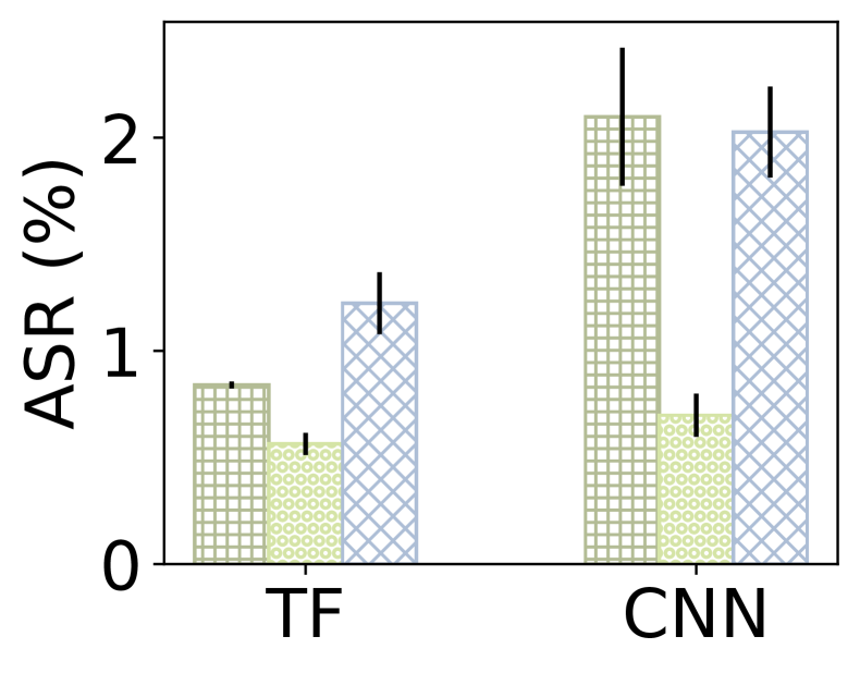
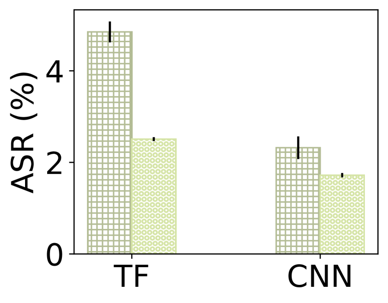
We compare four ways of robustification, ①: authentic adversarial-training, and iterative augmentation using ②: PGD’s samples, ③: PANTS’ samples, ④: Amoeba’s samples. ②, ③ and ④ share the same iterative way of robustification and the only difference is the method to generate adversarial samples. PANTS and Amoeba generate adversarial, semantic-preserving, and adversarial samples while PGD just generates adversarial samples. Figure 8 shows the accuracy and ASR of the robustfied ML models against end-host attackers under the application APP. Adversarially-trained models are robust against attacks from PANTS and Amoeba, but suffer from low accuracy. In contrast, iterative augmentation doesn’t drop the model accuracy, but not all of them can improve robustness for the model. PANTS-robustified models are more robust against both PANTS and Amoeba compared to the vanilla one. But Amoeba-robustified models can only be robust against Amoeba and PGD-robustified cannot be robust against any of the attacks.
Finding 3: PANTS improves the robustness of a model against any attack method 142% more than Amoeba


| PANTS | Amoeba | BAP | |
| PANTS | 57.65% | 49.98% | 50.52% |
| Amoeba | 20.89% | 36.89% | 7.50% |
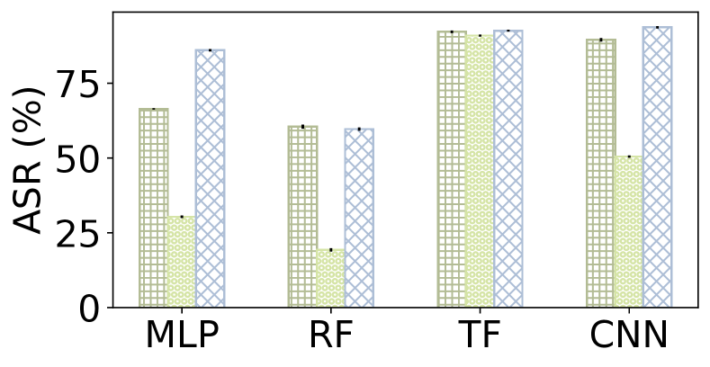
After robustification, we use again PANTS, Amoeba and BAP to re-attack (generate adversarial inputs for) the robustified models to re-evaluate models’ vulnerability. We train a new agent for Amoeba on to fool each robustified model . Figure 9 shows the ASR using PANTS, Amoeba, or BAP to find adversarial samples from the vanilla, PANTS, and Amoeba robustified models for the end-host threat model. ASR for the in-path threat model is shown in figure 11 in the Appendix. These results show that PANTS-robustified models are generally robust against the attack from PANTS, Amoeba and BAP, while Amoeba-robustified models are only robust against Amoeba. Table 2 shows the robustness improvement when robustified by PANTS and Amoeba and evaluated with PANTS, Amoeba and BAP. Robustness improvement is defined as . PANTS-robustified models demonstrate 52.72% robustness improvement on average while Amoeba-robustified ones only demonstrate 21.76%. PANTS-robustified models can have 142% more robustness improvement than Amoeba-robustified ones.
Prior works, especially in RL, have found that adversarial training can only defend a model against adversarial samples generated by the same generation process as the one used in training [37]. However, we found that augmenting with a large number of adversarial, realizable and semantics-preserving samples has the potential to robustify the model against multiple different attacks. That is the case because the space of adversarial, realizable, and semantics-preserving samples (generated by PANTS) is smaller than the space of samples that are only adversarial.
PANTS-robustified models demonstrate considerable robustness improvement against PANTS, Amoeba and BAP. However, we do not claim that PANTS-robustified models are robust against any possible attacks. First, the ASR for PANTS-robustified models doesn’t drop to 0, meaning that these attack methods can still find adversarial samples against the robustified models. Second, as an empirical way of robustification, we don’t have a theoretical guarantee that the robustified models are robust against the full spectrum of perturbation. Figure 11(f) shows that there still exists at least one such that the PANTS-robustified model doesn’t provide enough robustness. Still, this work presents a clear, extendible move towards the right direction.
Finding 4: Transferability provides an opportunity to robustify a MNC without white-box access.

There are use cases in which a network operator will not have access to the MNC, e.g., because the MNC is designed by a third party and its details are secret. While this is not our target setting, we show that transferability of adversarial samples PANTS might be able to help the network operator e.g., by providing examples in which the target MNC misclassified or by providing potentially intresting test cases for the MNC designer.
Transferability is defined as the ratio of adversarial samples that are generated for a given implementation of ML classifier that can also be adversarial against another one. Concretely, suppose we evaluate transferability of the adversarial samples generated from to , we first construct the test set that both and can correctly classify. Then we use PANTS to generate adversarial samples for using and evaluate its adversariness against . Figure 10 shows the transferability result between MLP, RF, TF and CNN for end-host threat model tested for the application APP. Most of the transfer ASR is above 50%, showing that PANTS can be useful even without full access to the MNC implementation. To benefit from it the operator would need to train a proxy model and find adversarial samples against it using PANTS. According to Figure 10, the adversarial samples against the proxy model are likely to be adversarial against the target one. Note that the transfer ASR between different models cannot be compared directly. For example, the ASR of transferring adversarial samples from CNN to RF is 70.44% while directly attacking RF (transfer ASR from RF to RF) is 66.5%. This doesn’t necessarily mean that transferring CNN’s adversarial samples to RF is more effective than directly attacking RF directly attacking RF because transferring from CNN to RF is tested on while directly attack RF is tested on . As , the two tested datasets may not be identical.
6 Conclusion
This paper presents PANTS, a practical framework to help network operators evaluate and enhance the robustness of ML-powered networking classifiers. PANTS combines canonical AML methods, such as PGD, with an SMT solver to generate adversarial, realizable, and semantic-preserving packet sequences with a high success rate. Our comprehensive evaluation in three MNCs across multiple implementations shows that PANTS outperforms baselines in generating adversarial samples by 70% and 2X in ASR. Importantly, by integrating PANTS in an iterative adversarial training pipeline, we find that PANTS can robustify MNCs against various attack methodologies by 52.72% on average.
References
- [1] Adversarial-robustness-toolbox for scikit-learn randomforestclassifier. https://github.com/Trusted-AI/adversarial-robustness-toolbox/blob/main/notebooks/classifier_scikitlearn_RandomForestClassifier.ipynb.
- [2] Adversarial-robustness-toolbox for xgboost. https://github.com/Trusted-AI/adversarial-robustness-toolbox/blob/main/notebooks/classifier_xgboost.ipynb.
- [3] azure. https://azure.microsoft.com/.
- [4] scikit-learn. https://scikit-learn.org/stable/.
- [5] Shahad Alahmed, Qutaiba Alasad, Maytham M. Hammood, Jiann-Shiun Yuan, and Mohammed Alawad. Mitigation of black-box attacks on intrusion detection systems-based ml. Computers, 11(7), 2022.
- [6] Nagender Aneja, Sandhya Aneja, and Bharat Bhargava. Ai-enabled learning architecture using network traffic traces over iot network: A comprehensive review. Wireless Communications and Mobile Computing, 2023:8658278, Feb 2023.
- [7] Pin-Yu Chen, Huan Zhang, Yash Sharma, Jinfeng Yi, and Cho-Jui Hsieh. Zoo: Zeroth order optimization based black-box attacks to deep neural networks without training substitute models. In Proceedings of the 10th ACM workshop on artificial intelligence and security, pages 15–26, 2017.
- [8] Jacob Devlin. Bert: Pre-training of deep bidirectional transformers for language understanding. arXiv preprint arXiv:1810.04805, 2018.
- [9] Edsger Wybe Dijkstra. A Discipline of Programming. Prentice Hall PTR, USA, 1st edition, 1997.
- [10] Rohan Doshi, Noah Apthorpe, and Nick Feamster. Machine learning ddos detection for consumer internet of things devices. In 2018 IEEE Security and Privacy Workshops (SPW), pages 29–35, 2018.
- [11] Gerard Draper-Gil, Arash Habibi Lashkari, Mohammad Saiful Islam Mamun, and Ali A. Ghorbani. Characterization of encrypted and vpn traffic using time-related features. In Proceedings of the 2nd International Conference on Information Systems Security and Privacy, pages 407–414, 2016. https://doi.org/10.5220/0005740704070414.
- [12] Dmitry Duplyakin, Robert Ricci, Aleksander Maricq, Gary Wong, Jonathon Duerig, Eric Eide, Leigh Stoller, Mike Hibler, David Johnson, Kirk Webb, Aditya Akella, Kuangching Wang, Glenn Ricart, Larry Landweber, Chip Elliott, Michael Zink, Emmanuel Cecchet, Snigdhaswin Kar, and Prabodh Mishra. The design and operation of CloudLab. In 2019 USENIX Annual Technical Conference (USENIX ATC 19), pages 1–14, Renton, WA, July 2019. USENIX Association.
- [13] Robert W Floyd. Assigning meanings to programs. In Program Verification: Fundamental Issues in Computer Science, pages 65–81. Springer, 1993.
- [14] Tomer Gilad, Nathan H. Jay, Michael Shnaiderman, Brighten Godfrey, and Michael Schapira. Robustifying network protocols with adversarial examples. In Proceedings of the 18th ACM Workshop on Hot Topics in Networks, HotNets ’19, page 85–92, New York, NY, USA, 2019. Association for Computing Machinery.
- [15] Ian J Goodfellow, Jonathon Shlens, and Christian Szegedy. Explaining and harnessing adversarial examples. arXiv preprint arXiv:1412.6572, 2014.
- [16] Ian J Goodfellow, Jonathon Shlens, and Christian Szegedy. Explaining and harnessing adversarial examples. arXiv preprint arXiv:1412.6572, 2014.
- [17] Julia Grabinski, Paul Gavrikov, Janis Keuper, and Margret Keuper. Robust models are less over-confident. Advances in Neural Information Processing Systems, 35:39059–39075, 2022.
- [18] Yuqiang Heng, Vikram Chandrasekhar, and Jeffrey G. Andrews. Utmobilenettraffic2021: A labeled public network traffic dataset. IEEE Networking Letters, 3(3):156–160, 2021.
- [19] Junchen Jiang, Rajdeep Das, Ganesh Ananthanarayanan, Philip A Chou, Venkata Padmanabhan, Vyas Sekar, Esbjorn Dominique, Marcin Goliszewski, Dalibor Kukoleca, Renat Vafin, et al. Via: Improving internet telephony call quality using predictive relay selection. In Proceedings of the 2016 ACM SIGCOMM Conference, pages 286–299. ACM, 2016.
- [20] Junchen Jiang, Vyas Sekar, Henry Milner, Davis Shepherd, Ion Stoica, and Hui Zhang. Cfa: A practical prediction system for video qoe optimization. In NSDI, pages 137–150, 2016.
- [21] Xi Jiang, Shinan Liu, Aaron Gember-Jacobson, Arjun Nitin Bhagoji, Paul Schmitt, Francesco Bronzino, and Nick Feamster. Netdiffusion: Network data augmentation through protocol-constrained traffic generation. Proc. ACM Meas. Anal. Comput. Syst., 8(1), feb 2024.
- [22] Minhao Jin. Improving managed network services using cooperative synthetic data augmentation. 2022.
- [23] Rakesh Kumar, Mayank Swarnkar, Gaurav Singal, and Neeraj Kumar. Iot network traffic classification using machine learning algorithms: An experimental analysis. IEEE Internet of Things Journal, 9(2):989–1008, 2022.
- [24] Linyi Li, Tao Xie, and Bo Li. Sok: Certified robustness for deep neural networks. In 2023 IEEE symposium on security and privacy (SP), pages 1289–1310. IEEE, 2023.
- [25] Xinjie Lin, Gang Xiong, Gaopeng Gou, Zhen Li, Junzheng Shi, and Jing Yu. Et-bert: A contextualized datagram representation with pre-training transformers for encrypted traffic classification. In Proceedings of the ACM Web Conference 2022, pages 633–642, 2022.
- [26] Haoyu Liu, Alec F. Diallo, and Paul Patras. Amoeba: Circumventing ml-supported network censorship via adversarial reinforcement learning. In Proceedings of the 13th International Conference on emerging Networking EXperiments and Technologies (CoNEXT), 2023.
- [27] Aleksander Madry, Aleksandar Makelov, Ludwig Schmidt, Dimitris Tsipras, and Adrian Vladu. Towards deep learning models resistant to adversarial attacks. arXiv preprint arXiv:1706.06083, 2017.
- [28] Jay Nandy, Sudipan Saha, Wynne Hsu, Mong Li Lee, and Xiao Xiang Zhu. Towards bridging the gap between empirical and certified robustness against adversarial examples. arXiv preprint arXiv:2102.05096, 2021.
- [29] Milad Nasr, Alireza Bahramali, and Amir Houmansadr. Defeating DNN-Based traffic analysis systems in Real-Time with blind adversarial perturbations. In 30th USENIX Security Symposium (USENIX Security 21), pages 2705–2722. USENIX Association, August 2021.
- [30] Xiao Peng, Weiqing Huang, and Zhixin Shi. Adversarial attack against dos intrusion detection: An improved boundary-based method. In 2019 IEEE 31st International Conference on Tools with Artificial Intelligence (ICTAI), pages 1288–1295, 2019.
- [31] Hadi Salman, Andrew Ilyas, Logan Engstrom, Ashish Kapoor, and Aleksander Madry. Do adversarially robust imagenet models transfer better? Advances in Neural Information Processing Systems, 33:3533–3545, 2020.
- [32] Rahul Anand Sharma, Ishan Sabane, Maria Apostolaki, Anthony Rowe, and Vyas Sekar. Lumen: a framework for developing and evaluating ml-based iot network anomaly detection. In Proceedings of the 18th International Conference on emerging Networking EXperiments and Technologies, pages 59–71, 2022.
- [33] Taveesh Sharma, Tarun Mangla, Arpit Gupta, Junchen Jiang, and Nick Feamster. Estimating webrtc video qoe metrics without using application headers. In Proceedings of the 2023 ACM on Internet Measurement Conference, pages 485–500, 2023.
- [34] Payap Sirinam, Mohsen Imani, Marc Juarez, and Matthew Wright. Deep fingerprinting: Undermining website fingerprinting defenses with deep learning. In Proceedings of the 2018 ACM SIGSAC conference on computer and communications security, pages 1928–1943, 2018.
- [35] Robin Sommer and Vern Paxson. Outside the closed world: On using machine learning for network intrusion detection. In 2010 IEEE Symposium on Security and Privacy, pages 305–316, 2010.
- [36] Vincent Tjeng, Kai Xiao, and Russ Tedrake. Evaluating robustness of neural networks with mixed integer programming. arXiv preprint arXiv:1711.07356, 2017.
- [37] Tom Tseng, Euan McLean, Kellin Pelrine, Tony T Wang, and Adam Gleave. Can go ais be adversarially robust? arXiv preprint arXiv:2406.12843, 2024.
- [38] Kai Wang, Zhiliang Wang, Dongqi Han, Wenqi Chen, Jiahai Yang, Xingang Shi, and Xia Yin. Bars: Local robustness certification for deep learning based traffic analysis systems.
- [39] Shiqi Wang, Huan Zhang, Kaidi Xu, Xue Lin, Suman Jana, Cho-Jui Hsieh, and J Zico Kolter. Beta-crown: Efficient bound propagation with per-neuron split constraints for neural network robustness verification. Advances in Neural Information Processing Systems, 34:29909–29921, 2021.
- [40] Eric Wong, Leslie Rice, and J Zico Kolter. Fast is better than free: Revisiting adversarial training. arXiv preprint arXiv:2001.03994, 2020.
- [41] Kaidi Xu, Zhouxing Shi, Huan Zhang, Yihan Wang, Kai-Wei Chang, Minlie Huang, Bhavya Kailkhura, Xue Lin, and Cho-Jui Hsieh. Automatic perturbation analysis for scalable certified robustness and beyond. Advances in Neural Information Processing Systems, 33:1129–1141, 2020.
- [42] Greg Yang, Tony Duan, J Edward Hu, Hadi Salman, Ilya Razenshteyn, and Jerry Li. Randomized smoothing of all shapes and sizes. In International Conference on Machine Learning, pages 10693–10705. PMLR, 2020.
- [43] Zhiyuan Yao, Yoann Desmouceaux, Mark Townsley, and Thomas Heide Clausen. Towards intelligent load balancing in data centers. CoRR, abs/2110.15788, 2021.
- [44] Yucheng Yin, Zinan Lin, Minhao Jin, Giulia Fanti, and Vyas Sekar. Practical gan-based synthetic ip header trace generation using netshare. In Proceedings of the ACM SIGCOMM 2022 Conference, SIGCOMM ’22, page 458–472, New York, NY, USA, 2022. Association for Computing Machinery.
Appendix A Features used in different applications
Different features are extracted from the feature engineering module among applications. Table 3 presents a summary of the features employed for each dataset. The selection of features is following the corresponding paper or the given script from the released dataset.
| Application | Features | |||||
| VPN Detection (VPN) |
|
|||||
|
|
|||||
|
|
Appendix B Hyperparemeters of ML models
To simplify the application setup, for each kind of ML classifier, we use the same architecture and hyperparameters for all the applications. The MLP is set with 4 hidden layers with 200 neurons each. It is trained with 500 epochs, and the optimizer is SGD. Since VPN detection is binary classification, a sigmoid function is used as the last activation layer, and the loss function is defined as binary cross entropy. Other applications are multi-class classification, hence we are using softmax function and the loss function is cross entropy. RF is implemented by Scikit-learn [4]. The maximum depth of trees is set as 12 and other parameters are set as default. The TF is borrowed from the idea of BERT [8]. It has 4 attention heads, 2 hidden layers and the intermediate size is 256. The CNN is derived from DF [34] which is previously designed for website fingerprinting. It has four sequential blocks where each includes two convolution layers and one max pooling layer, followed by three fully-connected layers. For both TF and CNN, only the first 400 packets for each packet sequence are encoded into the input. Packet sequences whose length are less than 400 will be padded with 0 for input format consistency. Both of them are trained with 200 epochs.
Appendix C Capability extension of Amoeba
For a fair comparison, we extend Amoeba’s capability to comply with the two evaluated threat models. First, we identify perturbable packets. Since the attacker’s capability can only perturb a single direction of packets instead of bi-direction, we modify the action function to work on either forward or backward packets. Then, we extend the action space of Amoeba to support more perturbations. The original action space has two features, representing the delay and the modified packet length of the given packet. We extend it by adding an integer to represent the number of injected packets after this packet. When the threat model assumes an end-host attacker, this newly added feature executes after each packet. We find that most of the adversarial samples generated by Amoeba are in conflict with the semantics constraints such as constraint of accumulative delay and maximum number of injected packets. We just add a hard budget to force the agent not to break this constraints. We found that this would help to improve Amoeba’s ASR compared to simply dropping all the adversarial sequences which break these flow-wise constraints. Further, for the applications that require multi-class classification, we modify the reward function. Amoeba’s original reward function only considers binary classification. Therefore, when targeting multi-class classification, we changed the reward function to cross-entropy. The agent can get a large reward when perturbing the original sample to cause misclassification.
Appendix D Testbed specification
For consistent evaluation, all the experiments using PANTS to generate adversarial samples are running on the cluster of Cloudlab machines [12]. Each machine has two Intel Xeon Silver 4114 10-core CPUs at 2.20 GHz and 192GB ECC DDR4-2666 memory. The rest of the experiments related to Amoeba rely on GPU training, which is running on two Azure machines [3]. Each one uses 16 vCPUs from AMD EPYC 7V12(Rome) CPU, 110GB memory, and an Nvidia Tesla T4 GPU with 16 GB GPU memory.
Appendix E Robustness of the PANTS- and Amoeba-robustified models
Figure 11 shows the robustness of using PANTS, Amoeba and BAP to attack PANTS- and Amoeba-robustified models under the in-path threat model.