PAGE: Domain-Incremental Adaptation with Past-Agnostic Generative Replay for Smart Healthcare
Abstract
Modern advances in machine learning (ML) and wearable medical sensors (WMSs) have enabled out-of-clinic disease detection. However, a trained ML model often suffers from misclassification when encountering non-stationary data domains after deployment. Use of continual learning (CL) strategies is a common way to perform domain-incremental adaptation while mitigating catastrophic forgetting. Nevertheless, most existing CL methods require access to previously learned domains through preservation of raw training data or distilled information. This is often infeasible in real-world scenarios due to storage limitations or data privacy, especially in smart healthcare applications. Moreover, it makes most existing CL algorithms inapplicable to deployed models in the field, thus incurring re-engineering costs. To address these challenges, we propose PAGE, a domain-incremental adaptation strategy with past-agnostic generative replay for smart healthcare. PAGE enables generative replay without the aid of any preserved data or information from prior domains. When adapting to a new domain, it exploits real data from the new distribution and the current model to generate synthetic data that retain the learned knowledge of previous domains. By replaying the synthetic data with the new real data during training, PAGE achieves a good balance between domain adaptation and knowledge retention. In addition, we incorporate an extended inductive conformal prediction (EICP) method into PAGE to produce a confidence score and a credibility value for each detection result. This makes the predictions interpretable and provides statistical guarantees for disease detection in smart healthcare applications. We demonstrate PAGE’s effectiveness in domain-incremental disease detection with three distinct disease datasets collected from commercially available WMSs. PAGE achieves highly competitive performance against state-of-the-art along with superior scalability, data privacy, and feasibility. Furthermore, PAGE is able to enable up to 75% reduction in clinical workload with the help of EICP. 222This work has been submitted to the ACM for possible publication. Copyright may be transferred without notice, after which this version may no longer be accessible. 333© 2024 ACM. Personal use of this material is permitted. Permission from ACM must be obtained for all other uses, in any current or future media, including reprinting/republishing this material for advertising or promotional purposes, creating new collective works, for resale or redistribution to servers or lists, or reuse of any copyrighted component of this work in other works.
1 Introduction
Physical and mental illnesses do not only affect our personal well-being but also impact global well-being. Especially after the overwhelming Coronavirus Disease 2019 (COVID-19) global pandemic, the world is seeking an efficient and effective strategy for disease detection. Thanks to the emergence of wearable medical sensors (WMSs) and modern advances in machine learning (ML), disease detection can now be made simple and accessible to not only health providers but also the general public, even in an out-of-clinic scenario [11, 49, 13, 2, 8, 36, 15, 44]. However, a trained ML model often misclassifies when it encounters input data outside of the underlying probability distribution it was trained on. For example, an ML model trained to detect diabetes with data collected from the elderly might be inaccurate in detecting diabetes in young adults. Therefore, if an ML model cannot perform domain-incremental adaptation to retain its disease-detection accuracy in new data domains, it would place the above-mentioned gains at risk.
Naively fine-tuning an ML model with data collected from new distributions degrades its performance on prior domains due to overfitting. This phenomenon in ML is well known as catastrophic forgetting (CF) [25, 30]. To alleviate CF, prior works have developed various continual learning (CL) strategies to perform domain-incremental adaptation while retaining learned knowledge [31, 24, 6, 26, 21]. These strategies include imposing restrictions on the update process of model parameters through regularization [16, 52, 20], dynamically reconfiguring model architectures to accommodate new tasks [22, 50, 38], and replaying exemplars from past tasks during training [32, 14, 37, 19]. However, most of the existing works focus on image-based CL tasks instead of nonstationary data distributions in tabular datasets. Tabular data are the most common data format for smart healthcare applications based on WMSs, such as physiological measurements and user demographics. Therefore, owing to the significant difference in their data modalities, the application of CL strategies to tabular data is still underexplored [18, 4].
On the other hand, most existing CL strategies require access to previously learned domains through preservation of either raw training data or distilled information [16, 52, 32, 19]. Nevertheless, the use of a patient’s personal health record is strictly regulated through numerous laws and regulations. Therefore, storing real patient data for exemplar replay in domain-incremental adaptation is often prohibited due to data privacy reasons. In addition, preserving raw data or distilled knowledge from all learned domains places a constraint on a system’s scalability owing to storage limitations. Moreover, requesting stored data or information from prior CL domains may make a CL strategy inapplicable to existing models in the field. It confines most existing CL methods to re-architecting a new model from scratch (from the first CL task). However, this is often infeasible in real-world scenarios due to re-engineering costs.
To address the aforementioned challenges, we propose PAGE, a domain-incremental adaptation strategy with past-agnostic generative replay. PAGE targets WMS tabular data in smart healthcare applications, such as physiological signals and demographic information. It adopts a generative replay CL method that features past-agnostic synthetic data generation (SDG). When adapting to new domains, PAGE does not rely on replaying raw preserved data or exploiting distilled information from learned domains to mitigate CF. Instead, it takes advantage of real data from new domains to generate synthetic data that retain learned knowledge for replay. In addition, we incorporate an extended inductive conformal prediction (EICP) method in PAGE. EICP enables PAGE to generate a confidence score and a credibility value for each disease-detection result with little computational overhead. This enables model interpretability by providing users with statistical guarantees on its predictions. We summarized the advantages of PAGE next.
-
1.
Scalability and privacy: PAGE has very low memory storage consumption since it does not store data or information from learned domains. Hence, PAGE is highly scalable to multi-domain disease detection while, at the same time, preserving patient privacy.
-
2.
Feasibility: PAGE features a past-agnostic replay paradigm. This makes any off-the-shelf model amenable to domain-incremental adaptation, without the need to re-engineer new models from scratch.
-
3.
Clinical workload reduction: PAGE provides interpretability to disease-detection results. It enables users or medical practitioners to investigate if further clinician intervention is needed. When the model predictions are associated with high model confidence scores and credibility values, clinical workload can be significantly reduced.
The rest of the article is organized as follows. Section 2 introduces related works on ML-driven disease detection based on WMSs and CL strategies, and provides background on probability density estimation and conformal prediction (CP). Section 3 presents problem definitions and evaluation metrics employed in our work. Section 4 gives details of our proposed strategy. Section 5 provides information on the disease datasets used in our experiments and implementation details. Section 6 presents the experimental results. Section 7 discusses the limitations of our strategy and possible future work. Finally, Section 8 concludes the article.
2 Related Works and Background
In this section, we discuss related works and background material that are helpful to understanding the rest of the article.
2.1 Machine Learning for Disease Detection with Wearable Medical Sensors
The evolution of WMSs and ML has enabled efficient, effective, and accessible disease-detection systems. For example, Alfian et al. [2] propose a personalized healthcare monitoring system based on Bluetooth Low Energy (BLE)-based sensor devices and ML classifiers for diabetic patients. They gather distinct vital sign data from users with commercial BLE-based sensors. Then, the system analyzes the data with a multilayer perceptron (MLP) for early diabetes detection and a long short-term memory for future blood glucose level prediction. Farooq et al. [8] introduce a cost-effective electrocardiography (ECG) sensor to obtain ECG waveforms from patients and use K-means clustering to classify various arrhythmia conditions. Shcherbak et al. [36] exploit commercial WMSs to collect motion data using designated exercises from test subjects and use ML classifiers to detect early-stage Parkinson’s disease. Himi et al. [15] construct a framework, called MedAi, that adopts a prototype smartwatch with eleven sensors to collect physiological signals from users and a random forest (RF) algorithm to predict numerous common diseases. Wang et al. [44] develop an RF-based diagnostic system to detect the sleep apnea syndrome by collecting human pulse wave signals and blood oxygen saturation levels with a photoplethysmography optical sensor. Hassantabar et al. propose CovidDeep [11] and MHDeep [13] to detect the SARS-CoV-2 virus/COVID-19 disease and mental health disorders based on physiological signals collected with commercial WMSs and smartphones. They employ a grow-and-prune algorithm to synthesize optimal deep neural network (DNN) architectures for disease detection. Similarly, Yin et al. build DiabDeep [49] with grow-and-prune synthesis to deliver DNN models with sparsely-connected layers or sparsely-recurrent layers for diabetes detection based on WMS data and patient demographics.
2.2 Continual Learning Algorithms
ML models suffer from performance degradation when presented with data from outside of the underlying domains they were trained on. Simply fine-tuning these models with new data results in CF. Therefore, researchers have been working on developing various algorithms to create more robust and general models. Domain adaptation [7, 10, 5] is a sub-field in ML research that aims to address the aforementioned problem. However, most works in this sub-field focus on making ML models generalize from a source domain to a target domain. They are inapplicable to incremental multi-domain adaptation scenarios. Hence, we turn to CL strategies that enable ML models to perform domain-incremental learning (adaptation) in real-world scenarios with nonstationary data domains. Numerous CL algorithms have been proposed in the literature. Recent CL algorithms can mainly be categorized into three groups: regularization-based, architecture-based, and replay-based [30, 31, 24, 6, 26, 21].
2.2.1 Regularization-based Methods
These methods use distilled information for data-driven regularization to impose restrictions on the model parameter update process to prevent performance degradation on past tasks. A canonical example is elastic weight consolidation (EWC) [16]. EWC quadratically penalizes parameters that are important to previously-learned tasks, when deviating from the learned values. The importance of model parameters is weighted by the diagonal of a preserved Fisher information matrix distilled from prior tasks.
Another example in this category is synaptic intelligence (SI) [52]. SI introduces intelligence in each synapse to allow it to estimate its own importance in solving a given task based on its update trajectory. Then, SI stores this information as the weighting parameter for its quadratic regularization function to decelerate the parameter update process in order to mitigate CF on previous tasks.
Beyond restricting the update process of important parameters, learning without forgetting (LwF) [20] draws inspiration from knowledge distillation to perform CL with a multi-headed DNN architecture. Before learning a new task, LwF records output responses to new data features from each output head of the current network to generate various sets of pseudo labels. Pairs of pseudo labels and new data features distill learned knowledge of prior tasks from each output head. When LwF learns a new task, it trains on the new data features and their ground-truth labels on a new output head. In the meantime, it uses different sets of pseudo labels and copies of new data features to regularize the update process of their corresponding output heads to mitigate CF on past tasks.
Our work and LwF use a similar strategy to take advantage of new data and produce pseudo labels to perform CL. The main differences are that LwF aims to solve class-incremental learning problems with a multi-headed DNN and uses identical copies of new data features with their given pseudo labels for regularization. Directly applying LwF to domain-incremental adaptation problems with single-headed models can confuse the models since they are trained on the same set of data yet with different labels. In contrast, PAGE uses new real data to generate synthetic data and pseudo labels to perform generative replay to avoid this confusion in the training process.
In summary, regularization-based methods address CF without storing raw exemplars but often require the preservation of distilled knowledge of prior tasks. Empirically, they do not achieve satisfactory performance under challenging CL settings [45] or complex datasets [47]. Thus, we do not adopt regularization-based CL algorithms in our strategy.
2.2.2 Architecture-based Methods
These methods modify model architectures in various ways to accommodate new tasks while retaining learned knowledge. For example, PackNet [22] interactively prunes the unimportant parameters after learning each task and retrains the spare connections for future tasks. In addition, it stores a parameter selection mask for each learned task to designate the connections reserved for the task at test time.
Dynamically expandable network (DEN) [50] learns new tasks by expanding the network capacity dynamically to synthesize a compact, overlapping, and knowledge-sharing structure. It uses a multi-stage process for CL. It first selects the relevant parameters from previous tasks to optimize. Then, it evaluates the loss on the new task after training. Once the loss exceeds a designated threshold, it expands network capacity and trains the expanded network with group sparsity regularization to avoid excessive growth.
On the other hand, SpaceNet [38] efficiently exploits a fixed-capacity sparse neural network. When learning a new task, it adopts an adaptive training method to train the network from scratch. This method reserves neurons that are important to learned tasks and produces sparse representations in the hidden layers for each learned task to reduce inter-task interference. Next, it effectively frees up unimportant neurons in the model to accommodate the new task.
Architecture-based methods perform CL by expanding or sparing model capacity for new tasks. However, they might require a large number of additional parameters, be more complex to train, and not be scalable to many tasks. Hence, they generally are not favorable to wearable edge devices. Accordingly, we do not implement architecture-based CL methods in our framework either.
2.2.3 Replay-based Methods
In general, replay-based methods store sampled exemplars from previous tasks in a small buffer or use generative models to generate synthetic samples that represent learned tasks. These samples are replayed when learning a new task to mitigate CF. For example, incremental classifier and representation learning (iCaRL) [32] selects groups of exemplars that best approximate their class centers in the latent feature space and stores them in a memory buffer. Then, it replays the stored samples with new data to perform nearest-mean-of-exemplars classification when learning a new class and at test time. In addition, it updates the memory buffer based on the distance between data instances in the latent feature space.
Other than storing raw exemplars, replay using memory indexing (REMIND) [14] imitates the hippocampal indexing theory by storing compressed data samples. It performs tensor quantization to efficiently store compressed representations of data instances from prior tasks for future replays. Therefore, it increases buffer memory efficiency and improves scalability of the framework.
On the other hand, deep generative replay [37] uses a generative adversarial network [9] as the generator to generate synthetic images that imitate images from previous tasks. It uses a task-solving model as a solver to generate labels for the synthetic images to represent the knowledge of the learned tasks. When learning a new task, it interleaves the synthetic images and their labels with new data to update the generator and solver networks together. Generating synthetic data as a substitution for storing real data can preserve data privacy and allow the model to access as much training data as required for exemplar replay.
Finally, DOCTOR [19] is a state-of-the-art framework that targets various CL scenarios in the tabular data domain for smart healthcare applications. It exploits a replay-style CL algorithm that features an efficient exemplar preservation method and an SDG generative replay module. It allows users to choose between storing real samples or generating synthetic data for future replays. In addition, DOCTOR adopts a multi-headed DNN that enables simultaneous multi-disease detection.
Generally, replay-based methods incur memory storage overhead to store exemplars and, hence, are not highly scalable. On the other hand, generative replay methods often require prior information to generate synthetic data. Therefore, it is challenging to apply these methods to existing models without re-engineering a new model from scratch. However, empirical results have demonstrated that they achieve the best performance trade-offs and are much stronger at alleviating CF than the other two methods, even when solving complex CL problems [26, 18, 17]. Therefore, we develop a generative replay CL algorithm that requires no preserved tabular data or information from prior tasks.
2.3 Probability Density Estimation
A function that describes the probability distribution of a continuous random variable is called a probability density function (PDF). It provides information about the likelihood of the random variable taking on a value within a specific interval. Probability density estimation methods are used to estimate the PDF of a continuous random variable based on observed data. These methods can be classified into two groups: parametric and non-parametric. In an ablation study presented in Section 6.3.1, we show that a parametric density estimation method performs better in our domain-incremental adaptation experiments with WMS data. Therefore, we implement the parametric density estimation method in PAGE.
Parametric density estimation assumes that a PDF belongs to a parametric family. Therefore, density estimation is transformed into estimating various parameters of the family. One common example of parametric density estimation is the Gaussian mixture model (GMM). Suppose there are independent and identically distributed (i.i.d.) samples drawn from an unknown univariate distribution at any given point . The estimated PDF of is represented as a mixture of Gaussian models in the form:
where is the observed variables, represents the parameters of the GMM, is the Gaussian model component, denotes the hidden state variable of , and symbolizes the hidden state variables that indicate the GMM assignment. The prior probability of each Gaussian model component can be written as:
Each Gaussian model component is a -dimensional multivariate Gaussian distribution with mean vector and covariance matrix in the form:
where is the determinant of the covariance matrix. Therefore, the PDF modeled by the GMM can be simplified as follows:
| (1) |
where represents the weight of the Gaussian model component and denotes the normal distribution.
2.4 Conformal Prediction
CP was first proposed in [33, 42]. It complements each prediction result with a measure of confidence and credibility. The confidence score gives a measurement of the model uncertainty on the prediction. The credibility value indicates how suitable the training data are for producing the prediction. The paradigm can adopt any ML algorithm as the prediction rule, such as a support-vector machine, ridge regression, or a neural network [35]. By measuring how unusual a prediction result is relative to others, CP provides a statistical guarantee to a prediction through the confidence score and credibility value.
The original CP uses transductive inference to generate prediction with the underlying ML algorithm and all seen samples. However, it is highly computationally inefficient. Therefore, an alternative CP method based on inductive inference was proposed to address this issue [29, 27, 28]. Here, we give an overview of the main concepts behind the transductive conformal prediction (TCP) and inductive conformal prediction (ICP) methods. For a more comprehensive description and statistical derivations, see [35, 43].
2.4.1 Transductive Conformal Prediction
For a classification task in a sample set , we are given a training set of examples , where each example is a pair of a feature vector and its target label . Our task is to predict the classification label for a new and unclassified vector , where . We know a priori the set of all possible class labels , assume all samples in are i.i.d.. Under the i.i.d. assumption, TCP provisionally iteratively assigns a class label as the true label of the new vector and updates the underlying ML algorithm accordingly. Next, it measures the likelihood of class label being the true label of the new vector through a p-value function .
A p-value function gives the p-value of a class label assignment to the new sample , denoted by . A p-value function needs to satisfy the following properties [29, 23]:
-
•
, and for all probability distributions on ,
-
•
is semi-computable from above.
TCP constructs a p-value function by measuring how distinct each sample is from all others, namely measuring the non-conformity of each sample.
The non-conformity score of each sample is calculated by a family of non-conformity measures: . Therefore, the non-conformity score of a sample can be formulated as:
which indicates how different is from the other samples in the bag . The non-conformity scores of all samples can then be used to compute the p-value of the class label assignment as:
2.4.2 Inductive Conformal Prediction
As mentioned in Section 2.4.1, TCP iteratively updates the prediction rule with each possible label assignment to calculate its corresponding p-value. In other words, for any new feature vector with possible class labels, TCP needs to retrain the underlying algorithm times. Next, TCP has to apply each updated prediction rule times to get the updated non-conformity scores for each seen sample to calculate the p-value of assignment . This requires a significant amount of computations to perform one inference. Hence, it makes TCP highly unsuitable for lifelong learning and algorithms that require a long training period.
To address the computational inefficiency, ICP was proposed in the literature [29, 27, 28]. ICP adopts the same general ideas as TCP but uses a different strategy to compute the non-conformity measure. It splits the training set into two smaller sets: the proper training set with samples and the calibration set with samples. The proper training set is used to train the underlying ML algorithm and establish the prediction rule. The calibration set is used to calculate the p-values of each possible class label for any new sample . More specifically, the non-conformity scores are calculated from the bag , which represents the degree of disagreement between the prediction rule built upon the bag and the true labels with the class assignment for . This way, the prediction rule only needs to be trained once. Similarly, the non-conformity scores of the samples in the calibration set only need to be computed once as well.
As a result, the p-value of each possible class label for , with ICP, can be given as:
| (2) |
Finally, ICP follows the same procedure as TCP to obtain the predicted label and generate its corresponding confidence score and credibility value, as described in Section 2.4.1.
3 Problem Definitions and Evaluation Metrics
Next, we define the problem and present the metrics used for evaluation.
3.1 Problem Definitions
CL is defined as training ML models on a series of tasks where non-stationary data domains, different classification classes, or distinct prediction tasks are presented sequentially [31, 46]. Therefore, CL problems are usually categorized into three scenarios: domain-, class-, and task-incremental learning [41]. In this work, we focus on the domain-incremental learning scenario for our disease-detection tasks.
Domain-incremental adaptation can be defined as the scenario where data from different probability distribution domains for the same prediction task become available sequentially. For example, data collected from different cities, countries, or age groups may become available incrementally for the same disease-detection task. Given a prediction task, we define a potentially infinite sequence of various domains as , where the -th domain is depicted by . and refer to the set of data features and their corresponding target labels for the -th class in domain . refers to the total number of classification classes for the prediction task. The objective of domain-incremental adaptation is to train an ML model , parameterized by , such that it can incrementally learn new data domains in and predict their labels without degrading performance on prior domains.
3.2 Evaluation Metrics
Several metrics are commonly used to evaluate CL algorithms in the literature, including average accuracy, average forgetting, backward transfer (BWT), and forward transfer [31, 21]. We report the average accuracy and average F1-score across all learned domains in our experimental results to validate PAGE’s effectiveness in domain-incremental adaptation for various disease-detection tasks. When reporting the average F1-score, we define true positives (negatives) as the unhealthy (healthy) instances correctly classified as disease-positive (healthy) and false positives (negatives) as the healthy (unhealthy) instances misclassified as disease-positive (healthy). In addition, we report BWT to evaluate how well PAGE mitigates CF. BWT measures how much a CL strategy impacts a model’s performance on previous tasks when learning a new one. For a model that has learned a total of tasks, BWT can be defined as:
where represents the model’s test accuracy for the -th task after continually learning tasks, and denotes the model’s test accuracy for the -th task after continually learning tasks.
4 The Past-Agnostic Generative-Replay Strategy
We detail our methodology next.

4.1 Strategy Overview
First, we provide an overview of the proposed PAGE strategy. Fig. 1 shows its schematic diagram. It is composed of three steps for performing domain-incremental adaptation and generating system outputs. For example, we use PAGE to learn a new data domain with an ML model that has learned domains for a disease-detection task using WMS data. PAGE passes the new real WMS data from through an SDG module to generate synthetic data that retains the knowledge learned from domains to . Next, the synthetic data are replayed together with the new real data to update the model in a generative replay fashion. Finally, PAGE uses the proposed EICP method to produce detection results and their corresponding confidence scores and credibility values.
Fig. 2 shows the top-level flowchart of the three steps of PAGE. In Step 1, as shown in Fig. 2(a), the SDG module exploits only the real training and validation data from the new domain to produce synthetic data for training and validation, respectively. In Step 2, depicted in Fig. 2(b), the synthetic data for training are replayed with the real training data from the new domain to update the model. During this process, PAGE also records the average training loss values of all training data for Step 3. In Step 3, illustrated in Fig. 2(c), EICP uses the real validation data from the new domain, the synthetic data generated for validation, the average training loss values, and the new data for detection as inputs. Finally, EICP generates detection results along with their corresponding confidence scores and credibility values to provide model interpretability and statistical guarantees to users.
Next, we dive into the details of each step of PAGE.


4.2 Synthetic Data Generation
The SDG module generates synthetic data that include pairs of synthetic data features and pseudo labels for replay, to retain knowledge of learned domains. We draw inspiration from a framework called TUTOR [12] to build our SDG module. First, the module models the joint multivariate probability distribution of the real data features from the new domain through a probability density estimation function. Next, it generates synthetic data features by sampling from the learned distribution. Then, it passes the synthetic data features to the current model and records the responses from the output softmax layer. It assigns these raw output probability distributions as pseudo labels of the synthetic data features. The pairs of synthetic data features and their pseudo labels effectively represent the knowledge of the previous domains that the model has learned so far. Therefore, we can replay the synthetic data during the model update process to retain the learned knowledge.
We adopt a multi-dimensional GMM as the probability density estimation function in our SDG module. The probability distribution of the real data features is modeled as a mixture of Gaussian models, as mentioned in Section 2.3. The PDF of the learned distribution can be expressed using Eq. (1). Note that previous works [11, 13, 12, 40] have already shown that GMM can recreate the probability distribution of real data and generate high-quality synthetic data. The generated synthetic data can then replace real data in the training process while achieving similar test accuracy. However, one drawback of this method lies in its learning complexity. To address this problem, we use the expectation-maximization (EM) algorithm to determine the GMM parameters [12]. The EM algorithm iteratively solves this optimization problem in the following two steps until convergence:
-
•
Expectation-step: Given the current parameters of the GMM and observations from the real training data, estimate the probability that belongs to each Gaussian model component .
-
•
Maximization-step: Find the new parameters that maximize the expectation derived from the expectation-step.
Algorithm 1 shows the pseudocode of the SDG module. It is important to note that the input real data features for training GMM and the input real data features for validating GMM refer to the real data features that are used to train and validate the underlying GMM, respectively. They do not stand for the real training data features and real validation data features from the new domain. The algorithm starts by initializing a set of Gaussian model components, ranging from 1 to a user-specified maximum number . Then, for each candidate number , the algorithm fits a GMM to the given with Gaussian model components. To determine the optimal total number of components , we use the Bayesian information criterion (BIC) [34] for model selection. BIC is a commonly used criterion in statistics to measure how well a model fits the underlying data. BIC favors models that have a good fit with fewer parameters and smaller complexity, which results in a smaller chance of overfitting [39]. The algorithm computes the BIC score bic() of each GMM to evaluate the quality of the model. To further avoid the risk of overfitting, we use this criterion with the given . A lower BIC score implies a better fit in model selection. Therefore, the number that minimizes this criterion is chosen as the optimal . This means that Gaussian models are required to model the probability distribution of . Then, the algorithm finalizes the optimal GMM with components to fit . Next, it samples a user-defined number of synthetic data features from . Finally, we pass to the current model and assign the raw output probability distributions from its softmax output layer as their pseudo labels .
We repeat this procedure twice to generate synthetic data for training and validation. When we generate the synthetic data for training , the inputs are and . When we generate the synthetic data for validation , the inputs are and .
4.3 Model Update
In this step, we update the model and record the average training loss values of all the training data, real and synthetic, for the next step. To update the model while mitigating CF, we replay the synthetic training data with the real training data from the new domain during training. Due to the difference in dataset sizes between the real and synthetic training data, the model might be biased toward the dataset with more data. To avoid the biased prediction problem, we sample the same number of data instances from each dataset to form each mini-batch to train the model. In other words, if we set the mini-batch size to , of the data are sampled from the real training data from the new domain while the other of the data are sampled from the synthetic training data.
Algorithm 2 demonstrates the pseudocode of the model update procedure. In the beginning, we initialize a vector to store the average training loss of each data instance used in the training process. In addition, we concatenate the real and synthetic validation data features () and their labels () to prepare validation data (, ) for model update. Then, we train the model for epochs with training data in a mini-batch size . Within each epoch, while data instances are not exhausted in both real training data (, ) and synthetic training data (, ), we sample data instances from (, ) and another from (, ) to form a mini-batch data (, ) to update the model parameters . For each data instance in (, ), we record the training loss value in a temporary vector . At the end of each epoch, we accumulate the training loss values of all training data instances in vector . Also, we store the current and the resulting performance on (, ). After updating the model for epochs, we assign the that maximizes performance on (, ) to the updated model . Finally, we obtain the average of the training loss values over epochs to retrieve the vector of average training loss values for all training data.


4.4 Extended Inductive Conformal Prediction
Next, we propose EICP, an extended version of the original ICP, to generate a detection result, confidence score, and credibility value for a new data instance. The new data instance can belong to any domain that the model has learned so far. Similar to the original ICP introduced in Section 2.4.2, we combine the real and synthetic training data into a proper training set to train the underlying ML model. Next, we use the real and synthetic validation data as a calibration set to calculate non-conformity scores. As opposed to ICP, we extend the calibration set by including a subset of the proper training set. By doing so, we strengthen the ability of the calibration set to perform CP based on the learned domains.
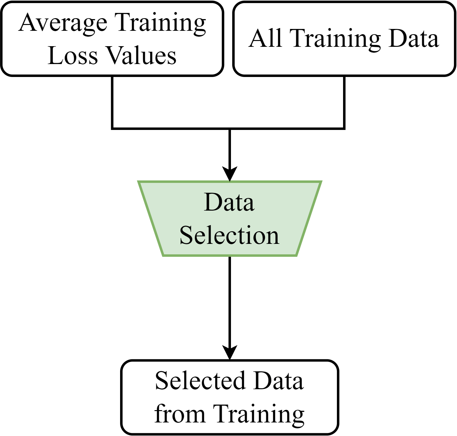
Fig. 3 shows the flowchart of EICP. It consists of three processes. In Process 1, EICP selects a subset of data from all training data, including the real and synthetic training data, to form the extended calibration set. As shown in Fig. 3(a), EICP selects the data through a data selection (DS) module based on their average training loss values. In Process 2, EICP computes the non-conformity scores of the extended calibration set through a non-conformity measure. As shown in Fig. 3(b), the softmax output responses of the extended calibration set from the updated model are used to compute their non-conformity scores. In Process 3, EICP first retrieves the softmax output response of the new data instance from the updated model and computes its non-conformity score using the non-conformity measure. Finally, as illustrated in Fig. 3(c), EICP produces the detection result for the new data instance, confidence score, and credibility value using the non-conformity scores of the new data instance and the calibration set through a p-value function, as described in Section 2.4.2.

4.4.1 Data Selection
We take inspiration from a framework called clustering training losses for label error detection (CTRL) [51] to construct the DS module. We look at the average training loss of each training data instance to evaluate how suitable the instance is for selection in the extended calibration set. Fig. 4 presents a graph of the training loss curves of the real training data in the CovidDeep dataset [11] across 150 epochs. The training loss values of some data instances decrease fast and stay near zero after around 30 epochs. As a result, these data instances have low average training loss values. They represent the easier-to-learn information in the given domain and, hence, are less non-conformal compared to other data. On the other hand, the training loss values of some data remain high until around 70 epochs. These data instances yield higher average training loss values and require more epochs for the model to learn. Therefore, they represent the difficult-to-learn knowledge in the underlying domain. These data are good candidates for helping EICP calibrate the non-conformity of a new data instance and its provisional class label assignment against the learned knowledge of the model. We conduct an ablation study for this design decision and give details in Section 6.3.3.
Algorithm 3 shows the pseudocode of the DS module. It starts by concatenating all training data, including the real training data (, ) and the synthetic training data (, ). Then, for each class label , the module sets an upper-level threshold and a lower-level threshold as the -th and the -th percentile of the average training loss values in , respectively. Next, the algorithm selects the data (, ) from the bag where data in () have average training loss values in that fall between the values of their corresponding and . Finally, the selected data (, ) are retrieved by concatenating all (, ). By doing so, the DS module selects the data for the extended calibration set in a stratified manner.
4.4.2 Non-Conformity Measure
Next, we calculate the non-conformity scores of the data in our extended calibration set, as described in Section 2.4.2. The extended calibration set includes the real validation data from the new domain, the synthetic data for validation, and the selected data from Process 2. We use their output responses from the updated model as inputs to the non-conformity measure. Next, we need to define a measure that captures the non-conformity of a prediction precisely.
Given a set of all possible class labels , the softmax output response of a model for a data feature is a probability distribution vector [] that corresponds to the probability distribution of its true label among , where . Therefore, for a data feature with a true class label , the higher the output probability of the true label, the more conforming the prediction is. On the contrary, the higher the other output probabilities , the less conforming the prediction is. Consequently, the most important output probability is the one with the maximum value except for the true label since it is the one that signifies model uncertainty.
We modify the function from [29] to define our non-conformity measure for a data feature with a provisional class label assignment as:
| (3) |
where . Parameter enables us to gain control over the sensitivity of the resulting non-conformity score based on the importance of the underlying output probability. By increasing , we reduce the importance of and increase the importance of all other output probabilities. Accordingly, we use Eq. (3) to compute the non-conformity scores of all data in our extended calibration set in this process.
4.4.3 p-Value Function
In this last process of EICP, we perform prediction for the given new data instance. Similar to Process 2, we pass the new data instance through the updated model to retrieve its output response. Then, we use its output probability distribution to compute its non-conformity score. Finally, we use the non-conformity scores from the extended calibration set and the new data instance to perform prediction with a p-value function. Based on the calculated p-values, we can produce a prediction result, confidence score, and credibility value for the new data instance.
Let our extended calibration set be with data instances. For a given new data instance with possible class labels , we compute the p-value of a provisional class label assignment as:
After computing all p-values for all possible ’s, we predict the class label of the new data instance as the one that yields the largest p-value. It can be written as:
Finally, for this prediction result, we output the confidence score as one minus the second largest p-value and the credibility value as the largest p-value. They are given as:
5 Experimental Setup
We describe the experimental setup next.
5.1 Datasets
We have chosen three different disease datasets collected from commercial WMSs to evaluate PAGE’s effectiveness in domain-incremental adaptation for disease detection. These are the CovidDeep [11], DiabDeep [49], and MHDeep [13] datasets from the literature. Data collection and experimental procedures for these datasets were governed by Institutional Review Board approval. The efficacy of these datasets has been validated by results presented in the literature [11, 49, 13, 19].
Table 1 shows the data features collected in the CovidDeep dataset. It contains various continuous physiological signals and Boolean responses to a simple questionnaire. The dataset was collected from 38 healthy individuals, 30 asymptomatic patients, and 32 symptomatic patients at San Matteo Hospital in Pavia, Italy. The data were acquired using commercial WMSs and devices, including an Empatica E4 smartwatch, a pulse oximeter, and a blood pressure monitor. Hassantabar et al. conducted numerous experiments [11] to identify which data features are the most beneficial to detecting COVID-19 in patients for obtaining a high disease-detection accuracy.
Table 2 shows the data features recorded in the DiabDeep dataset. It includes the physiological signals of participants and additional electromechanical and ambient environmental data. All data features have continuous values. The dataset was obtained from 25 non-diabetic individuals, 14 Type-I diabetic patients, and 13 Type-2 diabetic patients. While the physiological data were collected with an Empatica E4 smartwatch, other data were recorded using a Samsung Galaxy S4 smartphone. The additional smartphone data were proven to provide diagnostic insights through user habit tracking [48]. For instance, they help with body movement tracing and physiological signal calibration.
Table 2 also shows the data features recorded in the MHDeep dataset. It collects the same physiological signals and additional data features as those collected in the DiabDeep dataset. The dataset was obtained from 23 healthy participants, 23 participants with bipolar disorder, 10 participants with major depressive disorder, and 16 participants with schizoaffective disorder at the Hackensack Meridian Health Carrier Clinic, Belle Mead, New Jersey. As before, the data were collected using an Empatica E4 smartwatch and a Samsung Galaxy S4 smartphone.
| Data Features | Data Source | Data Type |
|---|---|---|
| Galvanic Skin Response () | ||
| Skin Temperature () | Smartwatch | Continuous |
| Inter-beat Interval () | ||
| Oxygen Saturation () | Pulse Oximeter | Continuous |
| Systolic Blood Pressure (mmHg) | Blood Pressure Monitor | Continuous |
| Diastolic Blood Pressure (mmHg) | Blood Pressure Monitor | Continuous |
| Immune-compromised | ||
| Chronic Lung Disease | ||
| Shortness of Breath | ||
| Cough | ||
| Fever | ||
| Muscle Pain | Questionnaire | Boolean |
| Chills | ||
| Headache | ||
| Sore Throat | ||
| Smell/Taste Loss | ||
| Diarrhea |
| Data Features | Data Source | Data Type |
| Galvanic Skin Response () | ||
| Skin Temperature () | ||
| Acceleration () | Smart Watch | Continuous |
| Inter-beat Interval () | ||
| Blood Volume Pulse | ||
| Humidity | ||
| Ambient Illuminance | ||
| Ambient Light Color Spectrum | ||
| Ambient Temperature | ||
| Gravity () | ||
| Angular Velocity () | ||
| Orientation () | Smart Phone | Continuous |
| Acceleration () | ||
| Linear Acceleration () | ||
| Air Pressure | ||
| Proximity | ||
| Wi-Fi Radiation Strength | ||
| Magnetic Field Strength |
5.2 Dataset Preprocessing
First, we preprocess all datasets to transform them into a suitable format for our experiments. We synchronize and window the data streams by dividing data into 15-second windows with 15-second shifts in between to avoid time correlation between adjacent data windows. Each 15-second window of data constitutes one data instance. Next, we flatten and concatenate the data within the same time window from the WMSs and smartphones. Then, we concatenate the sequential time series data with responses to the questionnaire for the CovidDeep dataset. This results in a total of 14047 data instances with 155 features each for the CovidDeep dataset, a total of 20957 data instances with 4485 features each for the DiabDeep dataset, and a total of 27082 data instances with 4485 features each for the MHDeep dataset. Subsequently, we perform min-max normalization on the feature data in all datasets to scale them into the range between 0 and 1. This prevents features with a wider value range from overshadowing those with a narrower range.
Next, we perform dimensionality reduction on the DiabDeep and MHDeep datasets using principal component analysis to reduce their dimension from 4485 to 155. First, we standardize the feature data in the datasets and compute the covariance matrix of the features. Then, we perform eigendecomposition to find the eigenvectors and eigenvalues of the covariance matrix to identify the principal components. Next, we sort the eigenvectors in descending order based on the magnitude of their corresponding eigenvalues. Finally, we construct a projection matrix to select the top 155 principal components. Afterward, we recast the data along the principal component axes to retrieve the 155-dimensional feature data for these datasets.
Due to the limited amount of patient data available in the datasets, we assume two different data domains in our domain-incremental adaptation experiments. For each dataset, we first randomly split the patients into two domains in a stratified fashion, where Domain 1 has 80% of the patients from each class and Domain 2 has the remaining 20%. Next, within each domain, we take the first 70%, the next 10%, and the last 20% of each patient’s sequential time series data to construct the training, validation, and test sets with no time overlap. Finally, we apply the Synthetic Minority Oversampling Technique (SMOTE) [3] to the partitioned training datasets to counteract the data imbalance issue within each dataset. We start by selecting a random data instance in a minority class and finding its five nearest neighbors in that class. Then, we randomly select one nearest neighbor from the five and draw a line segment between and in the feature space. Finally, we generate a synthetic data instance at a randomly selected point on the line segment between and . We then repeat this process until we obtain a balanced number of data instances in all classes in each partitioned training set.
5.3 Implementation Details
PAGE is applicable to any generic DNN model that performs classification on sequential time series data with a softmax output layer. For experimental simplicity, we use an MLP model to evaluate our PAGE strategy. We use grid search to obtain the best hyperparameter values for our MLP model, using the validation sets of the three datasets. We find that a four-layer architecture provides the optimal performance, in general. Fig. 5 shows the architecture of the final MLP model. It has an input layer with 155 neurons to align with the input dimensionality of the datasets. Subsequently, it has three hidden layers with 256, 128, and 128 neurons in each layer, respectively. Finally, it has an output layer with the number of neurons that corresponds to the number of possible classes. We use the rectified linear unit (ReLU) as the nonlinear activation function in the hidden layers and the softmax function for the output layer to generate the output probability distributions.

We use the stochastic gradient descent optimizer with a momentum of 0.9 in our experiments and initialize the learning rate to 0.005. We set the batch size to 128 for training, where data are drawn evenly from the real and synthetic training data, as described in Section 4.3. We train the MLP model for 300 epochs. We set the maximum number of Gaussian model components () for the SDG module to 10. In addition, based on the ablation study described in Section 6.3.2, we set the number of synthetic data instances () to 90% of the number of real data features for training GMM () in the new domain. In other words, the number of synthetic training (validation) data instances is 90% of the number of the new real training (validation) data instances. Similarly, based on the ablation study described in Section 6.3.3, we set the upper-level percentile () to the 90th percentile and the lower-level percentile () to the 70th percentile of the average training loss values of each classification class in the DS module in EICP. Finally, we set the parameter in Eq. (3) to 2.0 for our non-conformity measure.
We implement PAGE with PyTorch and perform the experiments on an NVIDIA A100 GPU. We employ CUDA and cuDNN libraries to accelerate the experiments.
6 Experimental Results
We present experimental results next.
| Datasets | Frameworks | Domain 1 | Domain 2 | F1-scoreavg | BWT | Buffer Size (MB) | |
|---|---|---|---|---|---|---|---|
| w/o Domain Adaptation | 0.977 | 0.808 | 0.893 | 0.930 | - | - | |
| Naive Fine-tuning | 0.767 | 1.000 | 0.884 | 0.929 | -0.217 | 0 | |
| Ideal Joint-training | 0.992 | 0.998 | 0.995 | 0.998 | 0.008 | 5.8 | |
| CovidDeep | DOCTOR | 0.979 | 1.000 | 0.990 | 0.994 | -0.007 | 1.7 |
| EWC | 0.844 | 1.000 | 0.922 | 0.958 | -0.125 | 0.7 | |
| LwF | 0.883 | 1.000 | 0.941 | 0.968 | -0.097 | 0 | |
| PAGE | 0.952 | 0.999 | 0.976 | 0.984 | -0.025 | 0 | |
| w/o Domain Adaptation | 0.921 | 0.368 | 0.645 | 0.647 | - | - | |
| Naive Fine-tuning | 0.445 | 1.000 | 0.723 | 0.796 | -0.477 | 0 | |
| Ideal Joint-training | 0.920 | 0.991 | 0.955 | 0.960 | -0.002 | 11.5 | |
| DiabDeep | DOCTOR | 0.918 | 0.995 | 0.957 | 0.961 | -0.004 | 3.4 |
| EWC | 0.648 | 0.958 | 0.803 | 0.822 | -0.280 | 0.7 | |
| LwF | 0.751 | 0.980 | 0.866 | 0.876 | -0.185 | 0 | |
| PAGE | 0.918 | 0.977 | 0.947 | 0.949 | -0.003 | 0 | |
| w/o Domain Adaptation | 0.824 | 0.108 | 0.466 | 0.753 | - | - | |
| Naive Fine-tuning | 0.280 | 0.986 | 0.633 | 0.794 | -0.554 | 0 | |
| Ideal Joint-training | 0.834 | 0.942 | 0.888 | 0.979 | -0.006 | 13.6 | |
| MHDeep | DOCTOR | 0.819 | 0.954 | 0.887 | 0.977 | -0.013 | 4.1 |
| EWC | 0.434 | 0.923 | 0.678 | 0.830 | -0.428 | 0.7 | |
| LwF | 0.577 | 0.936 | 0.757 | 0.883 | -0.262 | 0 | |
| PAGE | 0.782 | 0.928 | 0.855 | 0.954 | -0.050 | 0 |
6.1 Domain-Incremental Adaptation Experiments
First, we evaluate the performance of PAGE for domain-incremental adaptation on the datasets introduced in Section 5.1. We compare PAGE against five different strategies, including naive fine-tuning, ideal joint-training, DOCTOR [19], EWC [16], and LwF [20]. The naive fine-tuning method naively fine-tunes the MLP model with real training data from new domains without adopting any CL algorithm. The ideal joint-training method represents the ideal scenario where we have access to all training data from both past and new domains to train the MLP model with all data jointly. DOCTOR performs replay-style CL by either preserving raw training data from past domains or using data from previous domains to generate synthetic data for future replays. We report its best performance based on its two algorithms. EWC stores a Fisher information matrix for learned domains to weigh the importance of each model parameter. Then, it imposes a quadratic penalty on the update process of the important parameters. LwF distills the knowledge of learned domains with the pseudo labels given to the real training data from new domains. Then, it trains the model on the new real training data with both their pseudo and ground-truth labels.
Table 3 presents the domain-incremental adaptation experimental results for all three datasets. The results are reported on the real test data from both domains of all datasets. As shown in the first row for each dataset, the MLP model without domain adaptation performs poorly on data from the second domain and has a low average test accuracy. The naive fine-tuning method makes the MLP model overfit to the second domain and performs poorly on the first domain due to CF. PAGE outperforms the naive fine-tuning method and achieves superior results compared to EWC and LwF. While DOCTOR and the ideal joint-training method perform very well on domain-incremental adaptation and achieve high average test accuracy, they require a memory buffer that scales up with the number of new domains to preserve data from all seen domains. On the other hand, PAGE achieves very competitive results with negligible loss in average test accuracy without incurring the memory buffer cost and suffering from scalability issues.
| ICP | Correct | Incorrect | Correctness | Error Rate | EICP | Correct | Incorrect | Correctness | Error Rate | |
|---|---|---|---|---|---|---|---|---|---|---|
| Domain1 | Certain | 696 | 0 | 0.330 | 0 | Certain | 1386 | 0 | 0.656 | 0 |
| Uncertain | 1227 | 189 | Uncertain | 537 | 189 | |||||
| Domain2 | Certain | 243 | 0 | 0.349 | 0 | Certain | 520 | 0 | 0.746 | 0 |
| Uncertain | 454 | 0 | Uncertain | 177 | 0 |
| ICP | Correct | Incorrect | Correctness | Error Rate | EICP | Correct | Incorrect | Correctness | Error Rate | |
|---|---|---|---|---|---|---|---|---|---|---|
| Domain1 | Certain | 708 | 0 | 0.212 | 0 | Certain | 1321 | 0 | 0.395 | 0 |
| Uncertain | 2301 | 338 | Uncertain | 1688 | 338 | |||||
| Domain2 | Certain | 201 | 0 | 0.239 | 0 | Certain | 445 | 0 | 0.529 | 0 |
| Uncertain | 662 | 18 | Uncertain | 378 | 18 |
| ICP | Correct | Incorrect | Correctness | Error Rate | EICP | Correct | Incorrect | Correctness | Error Rate | |
|---|---|---|---|---|---|---|---|---|---|---|
| Domain1 | Certain | 785 | 18 | 0.181 | 0.004 | Certain | 1430 | 32 | 0.329 | 0.007 |
| Uncertain | 2556 | 986 | Uncertain | 1911 | 972 | |||||
| Domain2 | Certain | 30 | 2 | 0.028 | 0.002 | Certain | 230 | 2 | 0.214 | 0.002 |
| Uncertain | 961 | 82 | Uncertain | 761 | 82 |
6.2 Extended Inductive Conformal Prediction Experiments
At test time, users can input their pre-processed WMS data into PAGE and obtain the disease-detection results, confidence scores, and credibility values, as shown in Fig. 1. The confidence scores and credibility values can help users determine if their detection results are robust enough and whether clinical intervention is required. For healthy results with high confidence scores and credibility values, clinical intervention is not necessary. For disease-positive results with high confidence scores and credibility values, users can be alerted to seek medical treatments.
To demonstrate and evaluate the performance of EICP in PAGE against the original ICP, we report their performances in a confusion matrix format. Tables 4, 5, and 6 show the CP experimental results for the CovidDeep, DiabDeep, and MHDeep datasets, respectively. The results are reported on the real test data from both domains of all three datasets. The rows of the confusion matrices indicate whether the model is certain or uncertain about its detection results. We say that the model is certain when its confidence score and credibility value are higher than certain thresholds. We select the threshold values for each dataset based on their validation datasets. The confidence score threshold for all three datasets is 90%. The credibility value thresholds for the CovidDeep, DiabDeep, and MHDeep datasets are 70%, 85%, and 90%, respectively. The columns indicate whether the detection results are correct or incorrect. The detection result is correct when it correctly predicts the ground-truth label. We define two metrics to evaluate CP performance: correctness and error rate. Correctness is defined as the number of certain and correct detection results over the number of all test data instances. Error rate is defined as the number of certain but incorrect detection results over the number of all test data instances.
As shown in the tables, EICP achieves superior correctness compared to the original ICP with an identical error rate for both CovidDeep and DiabDeep datasets. For MHDeep, EICP outperforms ICP in correctness with only a 0.3% increase in the error rate for Domain 1. These results demonstrate that EICP reflects model uncertainty more precisely than ICP because of its smaller number of correct but uncertain results. EICP also provides a more accurate statistical guarantee for disease detection (correct and certain). In addition, the results show that EICP reduces clinical workload by up to 75% (based on the correctness metric).
6.3 Ablation Study
Next, we present the results of some ablation studies.
6.3.1 Probability Density Estimation Method
| Datasets | Frameworks | Domain 1 | Domain 2 | F1-scoreavg | BWT | Buffer Size (MB) | |
|---|---|---|---|---|---|---|---|
| CovidDeep | PAGE with GMM | 0.952 | 0.999 | 0.976 | 0.984 | -0.025 | 0 |
| PAGE with KDE | 0.904 | 0.981 | 0.942 | 0.970 | -0.079 | 0 | |
| DiabDeep | PAGE with GMM | 0.918 | 0.977 | 0.947 | 0.949 | -0.003 | 0 |
| PAGE with KDE | 0.689 | 0.871 | 0.780 | 0.806 | -0.239 | 0 | |
| MHDeep | PAGE with GMM | 0.782 | 0.928 | 0.855 | 0.954 | -0.050 | 0 |
| PAGE with KDE | 0.669 | 0.813 | 0.741 | 0.897 | -0.163 | 0 |
In this ablation study, we construct the SDG module with the non-parametric kernel density estimation (KDE) method. Then, we compare its performance in domain-incremental adaptation with the SDG module composed of the parametric GMM density estimation method.
For a mathematical background and introduction to KDE, see [12, 19]. Here, we follow DOCTOR [19] to construct the KDE SDG module. We use a similar algorithm to Algorithm 1 to generate synthetic training data () and synthetic validation data ().
As shown in Table 7, PAGE with GMM greatly outperforms PAGE with KDE in all metrics except that they both do not need a memory buffer. This is the reason we chose the GMM density estimation method to construct our SDG module in PAGE.
6.3.2 Amount of Synthetic Data for Replay


Next, we perform an ablation study of the amount of synthetic data required for PAGE to perform domain-incremental adaptation. Figs. 6(a), 6(b), and 6(c) show the ablation study results on the domain-incremental adaptation performance versus the amount of synthetic data used for replay for the three datasets. The axes in the figures denote curves for average accuracy, average F1-score, and BWT. The axes represent the amount of synthetic data as a percentage of the amount of the real data from the new domain. When the amount of synthetic data used for replay is around 90% of the real data from the new domain, PAGE achieves the highest average accuracy. When more synthetic data are generated for replay, the chance that the model overfits to past domains and underperforms on the new domain becomes higher, which might impact average accuracy. Therefore, we set the number of synthetic data instances () in SDG to 90% of the number of the real data instances from the new domain for replay in PAGE.
6.3.3 Data Selection Range
In this experiment, we investigate the ranges for setting the lower-level percentile () and the upper-level percentile () for the DS module when performing EICP. As described in Section 4.4.1, the DS module selects the data whose average training loss values are within the range of the -th and the -th percentiles in the vector of the average training loss values . We sweep the selected range, namely the pair of percentiles (, ), from (0th, 20th), (10th, 30th), , to (80th, 100th) to select the data from all the training data for the extended calibration set. Figs. 7(a), 7(b), and 7(c) show the ablation study results for EICP performance versus the selected range for the DS module for all three datasets. We plot the correctness and error rate curves for both domains in the figures. The axes depict the curves for the metrics. The axes represent the selected range depicted in terms of (, ). As can be seen, EICP correctness increases for both domains as we select a higher range of (, ) for all datasets. However, the error rates on both domains spike up in the th and th range for all datasets. Therefore, we set to the 70th percentile and to the 90th percentile in the DS module.


7 Discussions
The experimental results presented in Section 6 demonstrate that PAGE is able to perform domain-incremental adaptation for disease-detection tasks without the aid of any preserved data or information from prior domains. In addition, PAGE is able to provide model prediction interpretability and statistical guarantees for its detection results with the help of the proposed EICP method. However, the current version of PAGE only targets domain-incremental adaptation scenarios. In future work, we plan to expand its scope to class-incremental and task-incremental scenarios for smart healthcare applications. Moreover, it will be interesting to apply PAGE to natural language processing and image classification tasks.
8 Conclusion
We proposed PAGE, a domain-incremental adaptation strategy with past-agnostic generative replay. PAGE uses generative replay to perform domain-incremental adaptation while alleviating CF without the need for past knowledge in the form of preserved data or information. It makes PAGE highly scalable to multi-domain adaptation due to very low storage consumption. It also enables PAGE to protect patient privacy in disease-detection applications. Moreover, PAGE is directly applicable to off-the-shelf models for domain adapatation without the need for re-architecting new models from scratch. The proposed EICP method enables PAGE to complement prediction results with statistical guarantees and model prediction interpretability. This can help general users and medical practitioners determine whether further clinical intervention is required.
Acknowledgments
This work was supported by NSF under Grant No. CNS-1907381.
References
- [1]
- Alfian et al. [2018] Ganjar Alfian, Muhammad Syafrudin, Muhammad Fazal Ijaz, M. Alex Syaekhoni, Norma Latif Fitriyani, and Jongtae Rhee. 2018. A personalized healthcare monitoring system for diabetic patients by utilizing BLE-based sensors and real-time data processing. Sensors 18, 7 (2018).
- Chawla et al. [2002] Nitesh V. Chawla, Kevin W. Bowyer, Lawrence O. Hall, and W. Philip Kegelmeyer. 2002. SMOTE: Synthetic minority over-sampling technique. Journal of Artificial Intelligence Research 16 (Jun. 2002), 321–357.
- Cossu et al. [2021] Andrea Cossu, Antonio Carta, Vincenzo Lomonaco, and Davide Bacciu. 2021. Continual learning for recurrent neural networks: An empirical evaluation. Neural Networks 143 (2021), 607–627.
- Csurka [2017] Gabriela Csurka. 2017. Domain adaptation for visual applications: A comprehensive survey. arXiv: 1702.05374 (2017).
- De Lange et al. [2022] Matthias De Lange, Rahaf Aljundi, Marc Masana, Sarah Parisot, Xu Jia, Aleš Leonardis, Gregory Slabaugh, and Tinne Tuytelaars. 2022. A continual learning survey: Defying forgetting in classification tasks. IEEE Transactions on Pattern Analysis and Machine Intelligence 44, 7 (2022), 3366–3385.
- Farahani et al. [2021] Abolfazl Farahani, Sahar Voghoei, Khaled Rasheed, and Hamid R. Arabnia. 2021. A brief review of domain adaptation. In Advances in Data Science and Information Engineering. 877–894.
- Farooq et al. [2021] Aqeel Farooq, Mehdi Seyedmahmoudian, and Alex Stojcevski. 2021. A wearable wireless sensor system using machine learning classification to detect arrhythmia. IEEE Sensors Journal 21, 9 (2021), 11109–11116.
- Goodfellow et al. [2020] Ian Goodfellow, Jean Pouget-Abadie, Mehdi Mirza, Bing Xu, David Warde-Farley, Sherjil Ozair, Aaron Courville, and Yoshua Bengio. 2020. Generative adversarial networks. Commun. ACM 63, 11 (Oct. 2020), 139–144.
- HassanPour Zonoozi and Seydi [2023] Mahta HassanPour Zonoozi and Vahid Seydi. 2023. A survey on adversarial domain adaptation. Neural Processing Letters 55, 3 (2023), 2429–2469.
- Hassantabar et al. [2021] Shayan Hassantabar, Novati Stefano, Vishweshwar Ghanakota, Alessandra Ferrari, Gregory N. Nicola, Raffaele Bruno, Ignazio R. Marino, Kenza Hamidouche, and Niraj K. Jha. 2021. CovidDeep: SARS-CoV-2/COVID-19 test based on wearable medical sensors and efficient neural networks. IEEE Transactions on Consumer Electronics 67, 4 (2021), 244–256.
- Hassantabar et al. [2023] Shayan Hassantabar, Prerit Terway, and Niraj K. Jha. 2023. TUTOR: Training neural networks using decision rules as model priors. IEEE Transactions on Computer-Aided Design of Integrated Circuits and Systems 42, 2 (2023), 483–496.
- Hassantabar et al. [2022] Shayan Hassantabar, Joe Zhang, Hongxu Yin, and Niraj K. Jha. 2022. MHDeep: Mental health disorder detection system based on wearable sensors and artificial neural networks. ACM Transactions on Embedded Computing Systems 21, 6, Article 81 (Dec. 2022), 22 pages.
- Hayes et al. [2020] Tyler L. Hayes, Kushal Kafle, Robik Shrestha, Manoj Acharya, and Christopher Kanan. 2020. REMIND your neural network to prevent catastrophic forgetting. In Proceedings of the European Conference on Computer Vision. 466–483.
- Himi et al. [2023] Shinthi Tasnim Himi, Natasha Tanzila Monalisa, MD Whaiduzzaman, Alistair Barros, and Mohammad Shorif Uddin. 2023. MedAi: A smartwatch-based application framework for the prediction of common diseases using machine learning. IEEE Access 11 (2023), 12342–12359.
- Kirkpatrick et al. [2017] James Kirkpatrick, Razvan Pascanu, Neil Rabinowitz, Joel Veness, Guillaume Desjardins, Andrei A. Rusu, Kieran Milan, John Quan, Tiago Ramalho, Agnieszka Grabska-Barwinska, Demis Hassabis, Claudia Clopath, Dharshan Kumaran, and Raia Hadsell. 2017. Overcoming catastrophic forgetting in neural networks. Proceedings of the National Academy of Sciences 114, 13 (2017), 3521–3526.
- Knoblauch et al. [2020] Jeremias Knoblauch, Hisham Husain, and Tom Diethe. 2020. Optimal continual learning has perfect memory and is NP-hard. In Proceedings of the 37th International Conference on Machine Learning, Vol. 119. 5327–5337.
- Kwon et al. [2021] Young D. Kwon, Jagmohan Chauhan, Abhishek Kumar, Pan Hui, and Cecilia Mascolo. 2021. Exploring system performance of continual learning for mobile and embedded sensing applications. In Proceedings of the IEEE/ACM Symposium on Edge Computing. 319–332.
- Li and Jha [2023] Chia-Hao Li and Niraj K Jha. 2023. DOCTOR: A multi-disease detection continual learning framework based on wearable medical sensors. arXiv:2305.05738 (2023).
- Li and Hoiem [2018] Zhizhong Li and Derek Hoiem. 2018. Learning without forgetting. IEEE Transactions on Pattern Analysis and Machine Intelligence 40, 12 (2018), 2935–2947.
- Mai et al. [2022] Zheda Mai, Ruiwen Li, Jihwan Jeong, David Quispe, Hyunwoo Kim, and Scott Sanner. 2022. Online continual learning in image classification: An empirical survey. Neurocomputing 469 (2022), 28–51.
- Mallya and Lazebnik [2018] Arun Mallya and Svetlana Lazebnik. 2018. PackNet: Adding multiple tasks to a single network by iterative pruning. In Proceedings of the IEEE/CVF Conference on Computer Vision and Pattern Recognition. 7765–7773.
- Martin-Löf [1966] Per Martin-Löf. 1966. The definition of random sequences. Information and Control 9, 6 (1966), 602–619.
- McCaffary [2021] David McCaffary. 2021. Towards continual task learning in artificial neural networks: Current approaches and insights from neuroscience. arXiv: 2112.14146 (2021).
- McCloskey and Cohen [1989] Michael McCloskey and Neal J. Cohen. 1989. Catastrophic interference in connectionist networks: The sequential learning problem. In Psychology of Learning and Motivation. Vol. 24. 109–165.
- Mendez and Eaton [2023] Jorge A. Mendez and Eric Eaton. 2023. How to reuse and compose knowledge for a lifetime of tasks: A survey on continual learning and functional composition. arXiv: 2207.07730 (2023).
- Papadopoulos et al. [2002a] Harris Papadopoulos, Kostas Proedrou, Volodya Vovk, and Alex Gammerman. 2002a. Inductive confidence machines for regression. In Proceedings of the 13th European Conference on Machine Learning. 345–356.
- Papadopoulos et al. [2002b] Harris Papadopoulos, Vladimir Vovk, and Alex Gammerman. 2002b. Qualified predictions for large data sets in the case of pattern recognition. In Proceedings of the International Conference on Machine Learning and Applications. 159–163.
- Papadopoulos et al. [2007] Harris Papadopoulos, Volodya Vovk, and Alex Gammerman. 2007. Conformal prediction with neural networks. In Proceedings of the 19th IEEE International Conference on Tools with Artificial Intelligence, Vol. 2. 388–395.
- Parisi et al. [2019] German I. Parisi, Ronald Kemker, Jose L. Part, Christopher Kanan, and Stefan Wermter. 2019. Continual lifelong learning with neural networks: A review. Neural Networks 113 (2019), 54–71.
- Qu et al. [2021] Haoxuan Qu, Hossein Rahmani, Li Xu, Bryan Williams, and Jun Liu. 2021. Recent advances of continual learning in computer vision: An overview. arXiv: 2109.11369 (2021).
- Rebuffi et al. [2017] Sylvestre-Alvise Rebuffi, Alexander Kolesnikov, Georg Sperl, and Christoph H. Lampert. 2017. iCaRL: Incremental classifier and representation learning. In Proceedings of the IEEE Conference on Computer Vision and Pattern Recognition.
- Saunders et al. [1999] Craig Saunders, Alexander Gammerman, and Volodya Vovk. 1999. Transduction with confidence and credibility. In Proceedings of the 16th International Joint Conference on Artificial Intelligence. 722–726.
- Schwarz [1978] Gideon Schwarz. 1978. Estimating the dimension of a model. The Annals of Statistics 6, 2 (1978), 461–464.
- Shafer and Vovk [2008] Glenn Shafer and Vladimir Vovk. 2008. A tutorial on conformal prediction. Journal of Machine Learning Research 9, 3 (2008).
- Shcherbak et al. [2023] Aleksei Shcherbak, Ekaterina Kovalenko, and Andrey Somov. 2023. Detection and classification of early stages of Parkinson’s disease through wearable sensors and machine learning. IEEE Transactions on Instrumentation and Measurement 72 (2023), 1–9.
- Shin et al. [2017] Hanul Shin, Jung Kwon Lee, Jaehong Kim, and Jiwon Kim. 2017. Continual learning with deep generative replay. In Advances in Neural Information Processing Systems, Vol. 30.
- Sokar et al. [2021] Ghada Sokar, Decebal Constantin Mocanu, and Mykola Pechenizkiy. 2021. SpaceNet: Make free space for continual learning. Neurocomputing 439 (2021), 1–11.
- Stoica and Selen [2004] Petre Stoica and Yngve Selen. 2004. Model-order selection: A review of information criterion rules. IEEE Signal Processing Magazine 21, 4 (2004), 36–47.
- Terway and Jha [2023] Prerit Terway and Niraj K. Jha. 2023. REPAIRS: Gaussian mixture model-based completion and optimization of partially specified systems. ACM Transactions on Embedded Computing Systems 22, 4, Article 69 (Jul. 2023), 36 pages.
- van de Ven and Tolias [2019] Gido M. van de Ven and Andreas S. Tolias. 2019. Three scenarios for continual learning. arXiv: 1904.07734 (2019).
- Vovk et al. [1999] Volodya Vovk, Alexander Gammerman, and Craig Saunders. 1999. Machine-learning applications of algorithmic randomness. (1999).
- Vovk et al. [2005] Vladimir Vovk, Alexander Gammerman, and Glenn Shafer. 2005. Algorithmic learning in a random world. 29 (2005).
- Wang et al. [2023] Shaokui Wang, Weipeng Xuan, Ding Chen, Yexin Gu, Fuhai Liu, Jinkai Chen, Shudong Xia, Shurong Dong, and Jikui Luo. 2023. Machine learning assisted wearable wireless device for sleep apnea syndrome diagnosis. Biosensors 13, 4 (2023).
- Wang et al. [2022a] Zhen Wang, Liu Liu, Yajing Kong, Jiaxian Guo, and Dacheng Tao. 2022a. Online continual learning with contrastive vision transformer. In Proceedings of the European Conference on Computer Vision. 631–650.
- Wang et al. [2022b] Zifeng Wang, Zizhao Zhang, Chen-Yu Lee, Han Zhang, Ruoxi Sun, Xiaoqi Ren, Guolong Su, Vincent Perot, Jennifer Dy, and Tomas Pfister. 2022b. Learning to prompt for continual learning. In Proceedings of the IEEE/CVF Conference on Computer Vision and Pattern Recognition. 139–149.
- Wu et al. [2019] Yue Wu, Yinpeng Chen, Lijuan Wang, Yuancheng Ye, Zicheng Liu, Yandong Guo, and Yun Fu. 2019. Large scale incremental learning. In Proceedings of the IEEE/CVF Conference on Computer Vision and Pattern Recognition.
- Yin and Jha [2017] Hongxu Yin and Niraj K. Jha. 2017. A health decision support system for disease diagnosis based on wearable medical sensors and machine learning ensembles. IEEE Transactions on Multi-Scale Computing Systems 3, 4 (2017), 228–241.
- Yin et al. [2021] Hongxu Yin, Bilal Mukadam, Xiaoliang Dai, and Niraj K. Jha. 2021. DiabDeep: Pervasive diabetes diagnosis based on wearable medical sensors and efficient neural networks. IEEE Transactions on Emerging Topics in Computing 9, 3 (2021), 1139–1150.
- Yoon et al. [2017] Jaehong Yoon, Eunho Yang, Jeongtae Lee, and Sung Ju Hwang. 2017. Lifelong learning with dynamically expandable networks. arXiv: 1708.01547 (2017).
- Yue and Jha [2022] Chang Yue and Niraj K. Jha. 2022. CTRL: Clustering training losses for label error detection. arXiv: 2208.08464 (2022).
- Zenke et al. [2017] Friedemann Zenke, Ben Poole, and Surya Ganguli. 2017. Continual learning through synaptic intelligence. In Proceedings of the 34th International Conference on Machine Learning, Vol. 70. 3987–3995.