Page curve from dynamical branes in JT gravity

Let us consider general 2d topological gravity with $K$ dynamical anti-FZZT branes.³³3In this paper we will eventually restrict ourselves to the JT gravity case, but most parts of our formalism can be applied to other 2d gravities as well. It is described by the double scaling limit of the matrix integral

	$\displaystyle Z$	$\displaystyle=\int dHe^{-\operatorname{Tr}V(H)}\det(\xi+H)^{-K}$		(1)
		$\displaystyle=\int dHdQdQ^{\dagger}e^{-\operatorname{Tr}V(H)-\operatorname{Tr}Q^{\dagger}(\xi+H)Q}.$

Here $H$ and $Q$ are $N\times N$ hermitian and $N\times K$ complex matrices respectively. $\xi$ is a parameter characterizing the anti-FZZT brane, which is now taken to be common to all $K$ branes. The potential could have been normalized as

$\displaystyle\frac{1}{g_{\rm s}}V(H),$

(2)

where $g_{\rm s}$ is the genus counting parameter, so that the genus expansion is manifest. In this paper we include $g_{\rm s}^{-1}$ in $V$ for simplicity. In the double scaling limit, $N$ is sent to infinity and the potential turns into the effective potential. In this paper we will further take the ’t Hooft limit

$\displaystyle K\to\infty,~{}g_{\rm s}\to 0\quad\text{with}~{}~{}t\equiv g_{\rm s}K~{}~{}\text{fixed}$

(3)

and evaluate quantities in the planar approximation. That is, we will ignore all higher-order corrections of expansions in $g_{\rm s}$ and $K^{-1}$.

The matrices $H,Q$ are often denoted by their components $H_{ab}$, $Q_{ai}$, where $a,b=1,\ldots,N$ are “color” indices and $i,j=1,\ldots,K$ are “flavor” indices. The color degrees of freedom are used for describing bulk gravity while the flavor degrees of freedom are thought of as describing the interior partners of the early Hawking radiation. One can regard the matrix element $H_{ab}$ as

$\displaystyle H_{ab}=\langle a|H|b\rangle,$

(4)

where $H$ is a Hamiltonian operator and $\{|a\rangle\}_{a=1}^{N}$ form an orthonormal basis of the corresponding $N$ dimensional Hilbert space

$\displaystyle\langle a|b\rangle=\delta_{ab},\qquad 1=\sum_{a}|a\rangle\langle a|.$

(5)

For $i$th random vector variable $Q_{ai}$ we consider the (canonical) thermal pure quantum state Sugiura:2013pla ; Goto:2021mbt

$\displaystyle|\psi_{i}\rangle=\sum_{a}e^{-\frac{1}{2}\beta H}|a\rangle Q_{ai}=\sum_{a,b}|b\rangle(e^{-\frac{1}{2}\beta H})_{ba}Q_{ai}.$

(6)

Here $\beta$ is the inverse temperature, which is identified with the (renormalized) length of an asymptotic boundary in 2d gravity. $|\psi_{i}\rangle$ play the role of the black hole microstates.

To study the entropy, we will compute the average of overlaps such as $\langle\psi_{i}|\psi_{j}\rangle$. We define the average of ${\cal O}$ by

$$\langle\overline{{\cal O}}\rangle=\int dHdQdQ^{\dagger}e^{-\operatorname{Tr}V(H)-\operatorname{Tr}Q^{\dagger}(\xi+H)Q}{\cal O}.$$

(7)

Here the angle brackets $\langle\ \rangle$ represent averaging over the color degrees of freedom while the overline $\overline{\rule{10.00002pt}{0.0pt}\rule{0.0pt}{6.45831pt}}$ represents averaging over the flavor degrees of freedom. It is convenient to change the variable as

$\displaystyle Q=(\xi+H)^{-\frac{1}{2}}C,$

(8)

so that the new random variable $C$ obeys the Gaussian distribution

$$\langle\overline{{\cal O}}\rangle=\int dHdCdC^{\dagger}\det(\xi+H)^{-K}e^{-\operatorname{Tr}V(H)-\operatorname{Tr}C^{\dagger}C}{\cal O}.$$

(9)

Thus, in terms of $C$ the flavor average becomes nothing but the Gaussian average. Note that the determinant factor is recovered from the integration measure. On the other hand, the thermal pure quantum state (6) becomes (see also appendix D of Penington:2019kki )

$\displaystyle|\psi_{i}\rangle=\sum_{a,b}|b\rangle\bigl{[}e^{-\frac{1}{2}\beta H}(\xi+H)^{-\frac{1}{2}}\bigr{]}_{ba}C_{ai}.$

(10)

For our discussion it is convenient to express (10) as

$\displaystyle|\psi_{i}\rangle=\sum_{a,b}|b\rangle(\sqrt{A})_{ba}C_{ai}$

(11)

with

$\displaystyle A(H)=\frac{e^{-\beta H}}{\xi+H}.$

(12)

We then consider the overlaps such as

	$\displaystyle W_{ij}$	$\displaystyle\equiv\langle\psi_{i}|\psi_{j}\rangle=\sum_{a,b}A_{ab}C_{ai}^{*}C_{bj},$		(13)
	$\displaystyle W_{ij}W_{ji}$	$\displaystyle=|\langle\psi_{i}|\psi_{j}\rangle|^{2}=\sum_{a,b,a^{\prime},b^{\prime}}A_{ab}A_{b^{\prime}a^{\prime}}C_{ai}^{*}C_{bj}C_{a^{\prime}i}C_{b^{\prime}j}^{*}.$

Recall that the Gaussian average of $C$ can be computed by the Wick contraction

	$\displaystyle\overline{C_{ai}^{*}C_{bj}}$	$\displaystyle=\delta_{ab}\delta_{ij},$		(14)
	$\displaystyle\overline{C_{ai}^{*}C_{bj}C_{a^{\prime}i}C_{b^{\prime}j}^{*}}$	$\displaystyle=\delta_{ij}\delta_{ab}\delta_{a^{\prime}b^{\prime}}+\delta_{aa^{\prime}}\delta_{bb^{\prime}}.$

By using these formulas, the average of the overlaps (13) are given by

	$\displaystyle\overline{\langle\psi_{i}|\psi_{j}\rangle}$	$\displaystyle=\delta_{ij}\operatorname{Tr}A,$		(15)
	$\displaystyle\overline{|\langle\psi_{i}|\psi_{j}\rangle|^{2}}$	$\displaystyle=\delta_{ij}(\operatorname{Tr}A)^{2}+\operatorname{Tr}A^{2}.$

As discussed in Penington:2019kki , one can visualize the above computation (15) by drawing diagrams. For instance, $\langle\psi_{i}|\psi_{j}\rangle$ in (13) can be represented by the following diagram

$\displaystyle\leavevmode\hbox to271.14pt{\vbox to29.92pt{\pgfpicture\makeatletter\hbox{\hskip 104.9894pt\lower-11.78091pt\hbox to0.0pt{\pgfsys@beginscope\pgfsys@invoke{ }\definecolor{pgfstrokecolor}{rgb}{0,0,0}\pgfsys@color@rgb@stroke{0}{0}{0}\pgfsys@invoke{ }\pgfsys@color@rgb@fill{0}{0}{0}\pgfsys@invoke{ }\pgfsys@setlinewidth{0.4pt}\pgfsys@invoke{ }\nullfont\hbox to0.0pt{\pgfsys@beginscope\pgfsys@invoke{ }{{}} {}{{}}{}{{{}} {}{}{}{}{}{}{}{} }{}\pgfsys@moveto{0.0pt}{0.0pt}\pgfsys@moveto{1.13815pt}{0.0pt}\pgfsys@curveto{1.13815pt}{0.62859pt}{0.62859pt}{1.13815pt}{0.0pt}{1.13815pt}\pgfsys@curveto{-0.62859pt}{1.13815pt}{-1.13815pt}{0.62859pt}{-1.13815pt}{0.0pt}\pgfsys@curveto{-1.13815pt}{-0.62859pt}{-0.62859pt}{-1.13815pt}{0.0pt}{-1.13815pt}\pgfsys@curveto{0.62859pt}{-1.13815pt}{1.13815pt}{-0.62859pt}{1.13815pt}{0.0pt}\pgfsys@closepath\pgfsys@moveto{0.0pt}{0.0pt}\pgfsys@stroke\pgfsys@invoke{ } {}{{}}{} {}{}\pgfsys@beginscope\pgfsys@invoke{ }\pgfsys@setdash{3.0pt,3.0pt}{0.0pt}\pgfsys@invoke{ }{}\pgfsys@moveto{1.13815pt}{0.0pt}\pgfsys@lineto{45.52371pt}{0.0pt}\pgfsys@stroke\pgfsys@invoke{ } \pgfsys@invoke{\lxSVG@closescope }\pgfsys@endscope{}{{}}{}{{}}{}{{}}{}{}{}\pgfsys@beginscope\pgfsys@invoke{ }\pgfsys@setlinewidth{0.8pt}\pgfsys@invoke{ }{}\pgfsys@moveto{45.52371pt}{0.0pt}\pgfsys@curveto{68.28557pt}{11.38092pt}{102.42836pt}{-11.38092pt}{113.8093pt}{0.0pt}\pgfsys@stroke\pgfsys@invoke{ } \pgfsys@invoke{\lxSVG@closescope }\pgfsys@endscope{}{{}}{} {}{}\pgfsys@beginscope\pgfsys@invoke{ }\pgfsys@setdash{3.0pt,3.0pt}{0.0pt}\pgfsys@invoke{ }{}\pgfsys@moveto{113.8093pt}{0.0pt}\pgfsys@lineto{160.47118pt}{0.0pt}\pgfsys@stroke\pgfsys@invoke{ } \pgfsys@invoke{\lxSVG@closescope }\pgfsys@endscope{}{{}}{}{{{}} {}{}{}{}{}{}{}{} }{}\pgfsys@moveto{160.47118pt}{0.0pt}\pgfsys@moveto{161.60933pt}{0.0pt}\pgfsys@curveto{161.60933pt}{0.62859pt}{161.09976pt}{1.13815pt}{160.47118pt}{1.13815pt}\pgfsys@curveto{159.84259pt}{1.13815pt}{159.33302pt}{0.62859pt}{159.33302pt}{0.0pt}\pgfsys@curveto{159.33302pt}{-0.62859pt}{159.84259pt}{-1.13815pt}{160.47118pt}{-1.13815pt}\pgfsys@curveto{161.09976pt}{-1.13815pt}{161.60933pt}{-0.62859pt}{161.60933pt}{0.0pt}\pgfsys@closepath\pgfsys@moveto{160.47118pt}{0.0pt}\pgfsys@stroke\pgfsys@invoke{ } {}{{}}{}{{}}{}\pgfsys@moveto{-11.38092pt}{0.0pt}\pgfsys@stroke\pgfsys@invoke{ }\hbox{\hbox{{\pgfsys@beginscope\pgfsys@invoke{ }{{}{}{{{}{}}}{{}{}} {{}{{}}}{{}{}}{}{{}{}} { }{{{{}}\pgfsys@beginscope\pgfsys@invoke{ }\pgfsys@transformcm{1.0}{0.0}{0.0}{1.0}{-101.65639pt}{-2.9211pt}\pgfsys@invoke{ }\hbox{{\definecolor{pgfstrokecolor}{rgb}{0,0,0}\pgfsys@color@rgb@stroke{0}{0}{0}\pgfsys@invoke{ }\pgfsys@color@rgb@fill{0}{0}{0}\pgfsys@invoke{ }\hbox{{$\langle\psi_{i}|\psi_{j}\rangle=(C^{\dagger}AC)_{ij}=$}} }}\pgfsys@invoke{\lxSVG@closescope }\pgfsys@endscope}}} \pgfsys@invoke{\lxSVG@closescope }\pgfsys@endscope}}} {}{{}}{}{{}}{}\pgfsys@moveto{0.0pt}{0.0pt}\pgfsys@stroke\pgfsys@invoke{ }\hbox{\hbox{{\pgfsys@beginscope\pgfsys@invoke{ }{{}{}{{ {}{}}}{ {}{}} {{}{{}}}{{}{}}{}{{}{}} { }{{{{}}\pgfsys@beginscope\pgfsys@invoke{ }\pgfsys@transformcm{1.0}{0.0}{0.0}{1.0}{-1.72256pt}{3.533pt}\pgfsys@invoke{ }\hbox{{\definecolor{pgfstrokecolor}{rgb}{0,0,0}\pgfsys@color@rgb@stroke{0}{0}{0}\pgfsys@invoke{ }\pgfsys@color@rgb@fill{0}{0}{0}\pgfsys@invoke{ }\hbox{{$i$}} }}\pgfsys@invoke{\lxSVG@closescope }\pgfsys@endscope}}} \pgfsys@invoke{\lxSVG@closescope }\pgfsys@endscope}}} {}{{}}{}{{}}{}\pgfsys@moveto{160.47118pt}{0.0pt}\pgfsys@stroke\pgfsys@invoke{ }\hbox{\hbox{{\pgfsys@beginscope\pgfsys@invoke{ }{{}{}{{ {}{}}}{ {}{}} {{}{{}}}{{}{}}{}{{}{}} { }{{{{}}\pgfsys@beginscope\pgfsys@invoke{ }\pgfsys@transformcm{1.0}{0.0}{0.0}{1.0}{158.12593pt}{5.47743pt}\pgfsys@invoke{ }\hbox{{\definecolor{pgfstrokecolor}{rgb}{0,0,0}\pgfsys@color@rgb@stroke{0}{0}{0}\pgfsys@invoke{ }\pgfsys@color@rgb@fill{0}{0}{0}\pgfsys@invoke{ }\hbox{{$j$}} }}\pgfsys@invoke{\lxSVG@closescope }\pgfsys@endscope}}} \pgfsys@invoke{\lxSVG@closescope }\pgfsys@endscope}}} {}{{}}{}{{}}{}\pgfsys@moveto{22.76186pt}{0.0pt}\pgfsys@stroke\pgfsys@invoke{ }\hbox{\hbox{{\pgfsys@beginscope\pgfsys@invoke{ }{{}{}{{ {}{}}}{ {}{}} {{}{{}}}{{}{}}{}{{}{}} { }{{{{}}\pgfsys@beginscope\pgfsys@invoke{ }\pgfsys@transformcm{1.0}{0.0}{0.0}{1.0}{11.25258pt}{6.033pt}\pgfsys@invoke{ }\hbox{{\definecolor{pgfstrokecolor}{rgb}{0,0,0}\pgfsys@color@rgb@stroke{0}{0}{0}\pgfsys@invoke{ }\pgfsys@color@rgb@fill{0}{0}{0}\pgfsys@invoke{ }\hbox{{$(C^{\dagger})_{ia}$}} }}\pgfsys@invoke{\lxSVG@closescope }\pgfsys@endscope}}} \pgfsys@invoke{\lxSVG@closescope }\pgfsys@endscope}}} {}{{}}{}{{}}{}\pgfsys@moveto{79.6665pt}{0.0pt}\pgfsys@stroke\pgfsys@invoke{ }\hbox{\hbox{{\pgfsys@beginscope\pgfsys@invoke{ }{{}{}{{ {}{}}}{ {}{}} {{}{{}}}{{}{}}{}{{}{}} { }{{{{}}\pgfsys@beginscope\pgfsys@invoke{ }\pgfsys@transformcm{1.0}{0.0}{0.0}{1.0}{73.23479pt}{5.47743pt}\pgfsys@invoke{ }\hbox{{\definecolor{pgfstrokecolor}{rgb}{0,0,0}\pgfsys@color@rgb@stroke{0}{0}{0}\pgfsys@invoke{ }\pgfsys@color@rgb@fill{0}{0}{0}\pgfsys@invoke{ }\hbox{{$A_{ab}$}} }}\pgfsys@invoke{\lxSVG@closescope }\pgfsys@endscope}}} \pgfsys@invoke{\lxSVG@closescope }\pgfsys@endscope}}} {}{{}}{}{{}}{}\pgfsys@moveto{136.57115pt}{0.0pt}\pgfsys@stroke\pgfsys@invoke{ }\hbox{\hbox{{\pgfsys@beginscope\pgfsys@invoke{ }{{}{}{{ {}{}}}{ {}{}} {{}{{}}}{{}{}}{}{{}{}} { }{{{{}}\pgfsys@beginscope\pgfsys@invoke{ }\pgfsys@transformcm{1.0}{0.0}{0.0}{1.0}{130.12491pt}{6.56633pt}\pgfsys@invoke{ }\hbox{{\definecolor{pgfstrokecolor}{rgb}{0,0,0}\pgfsys@color@rgb@stroke{0}{0}{0}\pgfsys@invoke{ }\pgfsys@color@rgb@fill{0}{0}{0}\pgfsys@invoke{ }\hbox{{$C_{bj}$}} }}\pgfsys@invoke{\lxSVG@closescope }\pgfsys@endscope}}} \pgfsys@invoke{\lxSVG@closescope }\pgfsys@endscope}}} \pgfsys@invoke{\lxSVG@closescope }\pgfsys@endscope{}{}{}\hss}\pgfsys@discardpath\pgfsys@invoke{\lxSVG@closescope }\pgfsys@endscope\hss}}\lxSVG@closescope\endpgfpicture}}.$

(16)

The black thick curve labeled by the color matrix $A_{ab}$ corresponds to the asymptotic boundary of 2d spacetime while the dashed lines correspond to the flavor degrees of freedom $C,C^{\dagger}$. The gravitational path integral in the presence of branes is given by the matrix integral (9). One can easily see that the gravitational computations in eq. (2.10) and Figure 3 of Penington:2019kki agree with the first and the second lines of (15), respectively.

As explained in Penington:2019kki , the reduced density matrix of radiation is represented by the ensemble average of

$\displaystyle\varrho_{ij}=\frac{W_{ij}}{\sum_{i=1}^{K}W_{ii}}=\left(\frac{W}{\operatorname{Tr}W}\right)_{ij}.$

(17)

This is normalized as $\operatorname{Tr}\varrho=1$. Let us first consider the “purity” $\overline{\operatorname{Tr}\varrho^{2}}$ as an example. In the planar approximation, we can take the average of the numerator and the denominator of $\operatorname{Tr}\varrho^{2}$ independently

	$\displaystyle\overline{\operatorname{Tr}\varrho^{2}}\approx\frac{\overline{\operatorname{Tr}W^{2}}}{\overline{\operatorname{Tr}W}^{2}}$	$\displaystyle=\frac{K(\operatorname{Tr}A)^{2}+K^{2}\operatorname{Tr}A^{2}}{(K\operatorname{Tr}A)^{2}}$		(18)
		$\displaystyle=\frac{1}{K}+\frac{\operatorname{Tr}A^{2}}{(\operatorname{Tr}A)^{2}}.$

Similarly, the average of $\operatorname{Tr}\varrho^{n}$ is approximated as

$\displaystyle\overline{\operatorname{Tr}\varrho^{n}}\approx\frac{\overline{\operatorname{Tr}W^{n}}}{(\overline{\operatorname{Tr}W})^{n}}=\frac{\overline{\operatorname{Tr}W^{n}}}{(K\operatorname{Tr}A)^{n}}.$

(19)

$\overline{\operatorname{Tr}W^{n}}$ in the numerator can be computed by using the Wick contraction of $C$ and $C^{\dagger}$. In the planar approximation one obtains

	$\displaystyle\overline{\operatorname{Tr}W}$	$\displaystyle=K\operatorname{Tr}A,$		(20)
	$\displaystyle\overline{\operatorname{Tr}W^{2}}$	$\displaystyle=K(\operatorname{Tr}A)^{2}+K^{2}\operatorname{Tr}A^{2},$
	$\displaystyle\overline{\operatorname{Tr}W^{3}}$	$\displaystyle=K(\operatorname{Tr}A)^{3}+3K^{2}\operatorname{Tr}A^{2}\operatorname{Tr}A+K^{3}\operatorname{Tr}A^{3},$
	$\displaystyle\overline{\operatorname{Tr}W^{4}}$	$\displaystyle=K(\operatorname{Tr}A)^{4}+6K^{2}\operatorname{Tr}A^{2}(\operatorname{Tr}A)^{2}+2K^{3}(\operatorname{Tr}A^{2})^{2}+4K^{3}\operatorname{Tr}A^{3}\operatorname{Tr}A+K^{4}\operatorname{Tr}A^{4}.$

In fact, $\overline{\operatorname{Tr}W^{n}}$ can be computed efficiently by means of the generating function

$\displaystyle R(\lambda)=\operatorname{Tr}\frac{1}{\lambda-\varrho}=\sum_{n=0}^{\infty}\frac{\operatorname{Tr}\varrho^{n}}{\lambda^{n+1}}=\frac{K}{\lambda}+\sum_{n=1}^{\infty}\frac{\overline{\operatorname{Tr}W^{n}}}{\lambda^{n+1}(K\operatorname{Tr}A)^{n}}.$

(21)

In the planar approximation $R(\lambda)$ satisfies

$\displaystyle\lambda R(\lambda)=K+\sum_{n=1}^{\infty}\frac{R(\lambda)^{n}\operatorname{Tr}A^{n}}{(K\operatorname{Tr}A)^{n}}.$

(22)

This equation was derived diagrammatically in Penington:2019kki . We give an alternative derivation based on the saddle point method in appendix A. By plugging (21) into (22), $\overline{\operatorname{Tr}W^{n}}$ can be obtained recursively. In this way, in the planar approximation we obtain

$\displaystyle\langle\overline{\operatorname{Tr}\varrho^{n}}\rangle\approx\frac{1}{K^{n-1}}+\frac{n(n-1)}{2K^{n-2}}\frac{\langle\operatorname{Tr}A^{2}\rangle}{\langle\operatorname{Tr}A\rangle^{2}}+\cdots+\frac{n}{K}\frac{\langle\operatorname{Tr}A^{n-1}\rangle}{\langle\operatorname{Tr}A\rangle^{n-1}}+\frac{\langle\operatorname{Tr}A^{n}\rangle}{\langle\operatorname{Tr}A\rangle^{n}}.$

(23)

Thus, to compute $\langle\overline{\operatorname{Tr}\varrho^{n}}\rangle$ we need to evaluate

$\displaystyle\langle\operatorname{Tr}A^{n}\rangle=\int dHe^{-\operatorname{Tr}V(H)}\det(\xi+H)^{-K}\operatorname{Tr}A^{n}.$

(24)

We evaluate it in the double scaling limit. In the planar approximation we have only to consider the genus zero part. It can be expressed in terms of the leading-order density $\rho_{0}(E)$ of the eigenvalues of $H$. As we studied in Okuyama:2021eju , for Witten-Kontsevich topological gravity with general couplings $\{t_{k}\}\ (k\in{\mathbb{Z}}_{\geq 0})$, $\rho_{0}(E)$ is given by

$\displaystyle\rho_{0}(E)=\frac{1}{\sqrt{2}\pi g_{\rm s}}\int_{E_{0}}^{E}\frac{dv}{\sqrt{E-v}}\frac{\partial f(-v)}{\partial(-v)}$

(25)

with

$\displaystyle f(u):=\sum_{k=0}^{\infty}(\delta_{k,1}-t_{k})\frac{u^{k}}{k!}.$

(26)

The threshold energy $E_{0}$ is determined by the condition (the genus-zero string equation)

$\displaystyle f(-E_{0})=0.$

(27)

In this paper we consider JT gravity, which corresponds to a particular background $t_{k}=\gamma_{k}$ with Mulase:2006baa ; Dijkgraaf:2018vnm ; Okuyama:2019xbv ⁴⁴4Another way to obtain JT gravity is to take the $p\to\infty$ limit of the $(2,p)$ minimal string Seiberg:2019 ; Saad:2019lba . Entanglement entropy in this context was studied recently in Hirano:2021rzg .

$\displaystyle\gamma_{0}=\gamma_{1}=0,\quad\gamma_{k}=\frac{(-1)^{k}}{(k-1)!}\quad(k\geq 2).$

(28)

As we studied in Okuyama:2021eju , the effect of anti-FZZT branes, i.e. the insertion of $\det(\xi+H)^{-K}$ amounts to shifting the couplings $t_{k}$ of topological gravity as⁵⁵5This shift of couplings was first recognized in the theory of soliton equations Date:1982yeu and appears in various contexts of matrix models and related subjects. For more details, see Okuyama:2021eju and references therein.

$\displaystyle t_{k}=\gamma_{k}+t(2k-1)!!(2\xi)^{-k-\frac{1}{2}}.$

(29)

This is valid as long as ${\rm Re}\,\xi>0$. Here $t$ is the ’t Hooft coupling in (3). Thus, (24) is evaluated as

$\displaystyle\begin{aligned} \langle\operatorname{Tr}A^{n}\rangle&\approx\langle\operatorname{Tr}A^{n}\rangle^{g=0}\\ &=\int_{E_{0}}^{\infty}dE\rho_{0}(E)A(E)^{n},\\ &\equiv Z_{n},\end{aligned}$

(30)

where $\rho_{0}(E)$ is now evaluated in the background (29). In this background, (26) becomes

$\displaystyle f(u=-v)\equiv f(v,t)=\sqrt{v}I_{1}(2\sqrt{v})+\frac{t}{\sqrt{2\xi+2v}},$

(31)

where we have changed the variable as $v=-u$ for convenience and $I_{k}(z)$ denotes the modified Bessel function of the first kind. (25) then becomes

$\displaystyle\rho_{0}(E)=\frac{1}{\sqrt{2}\pi g_{\rm s}}\left(\int_{E_{0}}^{E}dv\frac{I_{0}(2\sqrt{v})}{\sqrt{E-v}}-\frac{t}{E+\xi}\sqrt{\frac{E-E_{0}}{2(E_{0}+\xi)}}\right).$

(32)

Note that in Okuyama:2021eju we calculated $\rho_{0}(E)$ for JT gravity in the presence of $K$ FZZT branes. The above $\rho_{0}(E)$ for anti-FZZT branes is essentially identical to this except the sign of the ’t Hooft coupling $t$. Note also that this expression of $\rho_{0}(E)$ is valid as long as $t$ is not greater than the critical value $t_{\rm c}$. We will explain this in section 3.1.

We emphasize that we have treated anti-FZZT branes as dynamical objects. More specifically, in (24) the color average is evaluated in the presence of the determinant factor $\det(\xi+H)^{-K}$ and as a consequence the deformed eigenvalue density (32) is used in (30). This is the main difference from the approach of Penington:2019kki , which is based on the probe brane approximation at genus-zero

	$\displaystyle\langle\operatorname{Tr}A^{n}\rangle_{\rm probe}\Big{|}_{g=0}$	$\displaystyle=\int dHe^{-\operatorname{Tr}V(H)}\operatorname{Tr}A^{n}\Big{|}_{g=0}$		(33)
		$\displaystyle=\int_{0}^{\infty}dE\rho_{0}^{\text{JT}}(E)A(E)^{n},$

where the original JT gravity density of state $\rho_{0}^{\text{JT}}(E)$ is given by

$\displaystyle\rho_{0}^{\text{JT}}(E)=\frac{\sinh(2\sqrt{E})}{\sqrt{2}\pi g_{\rm s}}.$

(34)

However, in Penington:2019kki the same ’t Hooft limit as ours (3) is used. As we argued in Okuyama:2021eju , in this limit the back-reaction of (anti-)FZZT branes cannot be ignored and the couplings $t_{k}$ are shifted due to the insertion of branes. As a consequence, the eigenvalue density is deformed from $\rho_{0}^{\text{JT}}(E)$ in (34) to $\rho_{0}(E)$ in (32). Thus we have to use the dynamical brane picture in this limit.

We saw in the last subsection that the ensemble averages of $\varrho$ in the planar approximation are expressed in terms of $Z_{n}$ in (30). On the other hand, the general expression (23) of $\langle\overline{\operatorname{Tr}\varrho^{n}}\rangle$ is rather complicated as a function of $n$ and it is difficult to apply the replica trick directly to (23) to calculate the entropy. Instead, as detailed in Penington:2019kki , we can study the entropy using the resolvent $R(\lambda)$ for $\varrho$ in (21). By substituting (30), the Schwinger-Dyson equation (22) for $R(\lambda)$ becomes

	$\displaystyle\lambda R(\lambda)$	$\displaystyle=K+\sum_{n=1}^{\infty}\frac{R(\lambda)^{n}}{(KZ_{1})^{n}}\int_{E_{0}}^{\infty}dE\rho_{0}(E)A(E)^{n}$		(35)
		$\displaystyle=K+\int_{E_{0}}^{\infty}dE\rho_{0}(E)\frac{w(E)R(\lambda)}{K-w(E)R(\lambda)},$

where we have defined

$\displaystyle w(E)=\frac{A(E)}{Z_{1}}.$

(36)

Following Penington:2019kki , we divide the integral in (35) into two pieces

	$\displaystyle\lambda R(\lambda)$	$\displaystyle=K+\int_{E_{0}}^{E_{K}}dE\rho_{0}(E)\frac{w(E)R(\lambda)}{K-w(E)R(\lambda)}+\int_{E_{K}}^{\infty}dE\rho_{0}(E)\frac{w(E)R(\lambda)}{K-w(E)R(\lambda)}$		(37)
		$\displaystyle\approx K+\int_{E_{0}}^{E_{K}}dE\rho_{0}(E)\frac{w(E)R(\lambda)}{K-w(E)R(\lambda)}+\lambda_{0}R(\lambda),$

where $\lambda_{0}$ and $E_{K}$ are defined by

	$\displaystyle\lambda_{0}$	$\displaystyle=\frac{1}{K}\int_{E_{K}}^{\infty}dE\rho_{0}(E)w(E),$		(38)
	$\displaystyle K$	$\displaystyle=\int_{E_{0}}^{E_{K}}dE\rho_{0}(E).$

By rewriting (37) as

$\displaystyle R(\lambda)=\frac{K}{\lambda-\lambda_{0}}+\frac{1}{\lambda-\lambda_{0}}\int_{E_{0}}^{E_{K}}dE\rho_{0}(E)\frac{w(E)R(\lambda)}{K-w(E)R(\lambda)},$

(39)

we can solve $R(\lambda)$ by the iteration starting from $R(\lambda)=K/(\lambda-\lambda_{0})$. As discussed in Penington:2019kki , the second order iteration gives

	$\displaystyle R(\lambda)$	$\displaystyle\approx\frac{K}{\lambda-\lambda_{0}}+\frac{1}{\lambda-\lambda_{0}}\int_{E_{0}}^{E_{K}}dE\rho_{0}(E)\frac{w(E)K(\lambda-\lambda_{0})^{-1}}{K-w(E)K(\lambda-\lambda_{0})^{-1}}$		(40)
		$\displaystyle=\frac{K}{\lambda-\lambda_{0}}+\frac{1}{\lambda-\lambda_{0}}\int_{E_{0}}^{E_{K}}dE\rho_{0}(E)\frac{w(E)}{\lambda-\lambda_{0}-w(E)}.$

Using (38), we find

	$\displaystyle R(\lambda)$	$\displaystyle=\frac{1}{\lambda-\lambda_{0}}\left[\int_{E_{0}}^{E_{K}}dE\rho_{0}(E)+\int_{E_{0}}^{E_{K}}dE\rho_{0}(E)\frac{w(E)}{\lambda-\lambda_{0}-w(E)}\right]$		(41)
		$\displaystyle=\int_{E_{0}}^{E_{K}}dE\rho_{0}(E)\frac{1}{\lambda-\lambda_{0}-w(E)}.$

The eigenvalue density $D(\lambda)$ of the density matrix $\varrho_{ij}$ is obtained from the discontinuity of $R(\lambda)$

$\displaystyle D(\lambda)=\frac{R(\lambda-\mathrm{i}0)-R(\lambda+\mathrm{i}0)}{2\pi\mathrm{i}}=\int_{E_{0}}^{E_{K}}dE\rho_{0}(E)\delta\bigl{(}\lambda-\lambda_{0}-w(E)\bigr{)}.$

(42)

Finally, the von Neumann entropy is given by

	$\displaystyle S$	$\displaystyle=-\int d\lambda D(\lambda)\lambda\log\lambda$		(43)
		$\displaystyle=-\int_{E_{0}}^{E_{K}}dE\rho_{0}(E)(\lambda_{0}+w(E))\log\bigl{(}\lambda_{0}+w(E)\bigr{)}.$

We will use this expression to study the Page curve numerically in section 4.

In the rest of this section let us make several comments on the above approximation. We can check that $D(\lambda)$ in (42) is normalized correctly

$\displaystyle\operatorname{Tr}\varrho^{0}=\int d\lambda D(\lambda)\cdot 1=\int_{E_{0}}^{E_{K}}dE\rho_{0}(E)=K,$

(44)

where we have used (38). We also find

	$\displaystyle\operatorname{Tr}\varrho$	$\displaystyle=\int d\lambda D(\lambda)\cdot\lambda=\int_{E_{0}}^{E_{K}}dE\rho_{0}(E)(\lambda_{0}+w(E))$		(45)
		$\displaystyle=K\lambda_{0}+\int_{E_{0}}^{E_{K}}dE\rho_{0}(E)w(E)$
		$\displaystyle=\int_{E_{K}}^{\infty}dE\rho_{0}(E)w(E)+\int_{E_{0}}^{E_{K}}dE\rho_{0}(E)w(E)$
		$\displaystyle=\int_{E_{0}}^{\infty}dE\rho_{0}(E)w(E)$
		$\displaystyle=\frac{1}{Z_{1}}\int_{E_{0}}^{\infty}dE\rho_{0}(E)A(E)=\frac{1}{Z_{1}}Z_{1}=1,$

where we have used (38).

$\lambda_{0}$ in (38) can be written as

	$\displaystyle\lambda_{0}$	$\displaystyle=\frac{1}{K}\int_{E_{0}}^{\infty}dE\rho_{0}(E)w(E)-\frac{1}{K}\int_{E_{0}}^{E_{K}}dE\rho_{0}(E)w(E)$		(46)
		$\displaystyle=\frac{1}{K}-\overline{w}_{K},$

where we have used (45) and defined

$\displaystyle\overline{w}_{K}\equiv\frac{1}{K}\int_{E_{0}}^{E_{K}}dE\rho_{0}(E)w(E)=\frac{\int_{E_{0}}^{E_{K}}dE\rho_{0}(E)w(E)}{\int_{E_{0}}^{E_{K}}dE\rho_{0}(E)}.$

(47)

That is, $\overline{w}_{K}$ is the average of $w(E)$ in the “post Page” subspace $E<E_{K}$. Thus the resolvent is written as

$\displaystyle R(\lambda)=\operatorname{Tr}\frac{1}{\lambda-\varrho}=\int_{E_{0}}^{E_{K}}dE\rho_{0}(E)\frac{1}{\lambda-\lambda(E)},$

(48)

where

$\displaystyle\lambda(E)=\frac{1}{K}+w(E)-\overline{w}_{K}.$

(49)

$\lambda(E)$ behaves as

$$\lambda(E)\approx\left\{\begin{aligned} &\frac{1}{K}\quad&(K\ll g_{\rm s}^{-1}),\\ &w(E)-\overline{w}_{K}\quad&(K\gg g_{\rm s}^{-1}).\end{aligned}\right.$$

(50)

This corresponds to Figure 6 in Penington:2019kki . Note that the density matrix $\varrho_{ij}$ is originally a matrix in the flavor space, but after taking the average the spectrum $\lambda(E)$ of $\varrho_{ij}$ is effectively written in terms of energy eigenvalues in the “color” space. We have to project quantities onto the “post Page” subspace $E<E_{K}$ to ensure that the number of total state is $K=\int_{E<E_{K}}dE\rho_{0}(E)$.

Let us first clarify the definition of the threshold energy $E_{0}$. In the last section we saw that $E_{0}$ is determined by the threshold energy condition (27). For JT gravity with anti-FZZT branes, $f$ is given by (31) and the condition (27) is written explicitly as

$\displaystyle\sqrt{E_{0}}I_{1}(2\sqrt{E_{0}})=-\frac{t}{\sqrt{2(E_{0}+\xi)}}.$

(51)

The threshold energy $E_{0}$ is determined as a real solution of this equation. Here, $t>0$ by definition and we take $\xi>0$ in order for the shift of the couplings (29) to be valid. We show the plots of both sides of the equation (51) in Figure 1.

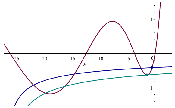We see that $\sqrt{E}I_{1}(2\sqrt{E})$ oscillates for $E<0$ and increases monotonically for $E>0$ starting from the origin, while $-t/\sqrt{2(E+\xi)}$ is always negative. Therefore $E_{0}$ has to be negative if it exists. However, the number of real solutions of (51) varies depending on the values of $t$ and $\xi$. In particular, (51) has no real solution when $t$ is very large, whereas it has multiple real solutions when $\xi$ is large and $t$ is small.⁶⁶6See also Johnson:2020lns for a similar problem in JT gravity with conical defects. On the other hand, one can easily see that (51) always has at least one real solution for sufficiently small $t$. We define $E_{0}$ as the largest real solution of (51) (i.e. the solution with the smallest absolute value), so that it is continuously deformed from $E_{0}=0$ for the original JT gravity case $t=0$.

As we see from Figure 1, $|E_{0}|$ is small for small $t$. If we increase $t$, $|E_{0}|$ also increases. Then there exists a critical point $t=t_{\rm c}$ beyond which $E_{0}$ no longer continues as a real solution. Thus, we expect a phase transition. This transition is qualitatively very similar to the one discussed in Gao:2021uro in the case of EOW branes. If one continuously increases $t$ beyond the critical point, $E_{0}$ and the second largest root turn into a pair of complex roots. It is therefore very likely that the saddle point of the matrix integral is described by an eigenvalue density with “Y” shaped support, similar to the one studied in Gao:2021uro . It would be interesting to study the model in this “Y” shaped phase further. In this paper we view this phase transition as the end of the black hole evaporation and focus on the physics before the phase transition.

At the critical value $t=t_{\rm c}$, the equation (51) has a double root $E_{0}^{\rm c}$. Thus $t_{\rm c}$ is determined by the condition

$\displaystyle f(E_{0}^{\rm c},t_{\rm c})=0,\quad\partial_{v}f(E_{0}^{\rm c},t_{\rm c})=0$

(52)

with $f(v,t)$ given in (31). Expanding the equation $f(E_{0},t)=0$ around $(v,t)=(E_{0}^{\rm c},t_{\rm c})$, we find

	$\displaystyle 0$	$\displaystyle=f(E_{0}^{\rm c},t_{\rm c})+\partial_{v}f(E_{0}^{\rm c},t_{\rm c})(E_{0}-E_{0}^{\rm c})+\frac{1}{2}\partial_{v}^{2}f(E_{0}^{\rm c},t_{\rm c})(E_{0}-E_{0}^{\rm c})^{2}$		(53)
		$\displaystyle\hskip 10.00002pt+\partial_{t}f(E_{0}^{\rm c},t_{\rm c})(t-t_{\rm c})+\cdots.$

The first two terms vanish due to (52). Thus, near $t=t_{\rm c}$ we find

$\displaystyle E_{0}-E_{0}^{\rm c}\approx C\sqrt{t_{\rm c}-t}\quad(t<t_{\rm c}),$

(54)

where $C$ is given by

$\displaystyle C=\sqrt{\frac{2\partial_{t}f(E_{0}^{\rm c},t_{\rm c})}{\partial_{v}^{2}f(E_{0}^{\rm c},t_{\rm c})}}.$

(55)

In Gao:2021uro , the effective zero-temperature entropy $S_{\text{eff}}$ was introduced. It is defined by the behavior of $\rho_{0}(E)$ near $E=E_{0}$:

$\displaystyle\rho_{0}(E)\sim e^{S_{\text{eff}}}\sqrt{E-E_{0}}.$

(56)

From (25) we find

	$\displaystyle e^{S_{\text{eff}}}$	$\displaystyle=\frac{\sqrt{2}}{\pi g_{\rm s}}\partial_{v}f(E_{0},t)$		(57)
		$\displaystyle=\frac{\sqrt{2}}{\pi g_{\rm s}}\left[I_{0}(2\sqrt{E_{0}})-\frac{t}{(2\xi+2E_{0})^{\frac{3}{2}}}\right].$

In Figure 2, we show the plot of $S_{\text{eff}}$. We see that $S_{\text{eff}}$ is a monotonically decreasing function of $t$.

Near $t=t_{\rm c}$, using (52) and (54) we find

$\displaystyle\begin{aligned} e^{S_{\text{eff}}}&\sim\partial_{v}f(E_{0},t)\\ &=\partial_{v}f(E_{0}^{\rm c},t_{\rm c})+\partial_{v}^{2}f(E_{0}^{\rm c},t_{\rm c})(E_{0}-E_{0}^{\rm c})+\partial_{t}\partial_{v}f(E_{0}^{\rm c},t_{\rm c})(t-t_{\rm c})+\cdots\\ &\sim\sqrt{t_{\rm c}-t}.\end{aligned}$

(58)

Using the above results, we can evaluate the critical behavior of the von Neumann entropy (43). It turns out that the critical behavior of the von Neumann entropy $S(t)$ in (43) is determined by that of the eigenvalue density near $E=E_{0}$

$\displaystyle\rho_{0}(E)\sim e^{S_{\text{eff}}}\sqrt{E-E_{0}}\sim\sqrt{t_{\rm c}-t}\sqrt{E-E_{0}}.$

(59)

One can show that the contribution of the $E$-integral (43) away from the edge $E=E_{0}$ is finite at $t=t_{\rm c}$. Subtracting this finite contribution and using (59) near $E=E_{0}$ in (43), we find

$\displaystyle S(t)-S(t_{\rm c})\sim\sqrt{t_{\rm c}-t}.$

(60)

In the next section we will confirm this behavior numerically.

We consider the von Neumann entropy (43) in JT gravity in the presence of $K$ anti-FZZT branes. As discussed in section 2 we compute the entropy for dynamical branes, but it is interesting to compute it in the probe brane approximation as well for the sake of comparison. In the probe brane approximation, we have $E_{0}=0$ and the eigenvalue density is given by $\rho_{0}^{\text{JT}}(E)$ in (34). We show the plot of the von Neumann entropy $S$ in Figure 3. We see that the entropy for the dynamical brane (solid blue curve) starts to decrease relative to the probe brane case (dashed orange curve). This is very similar to the Page curve of an evaporating black hole.

As we saw in the last section, we observe that the entropy exhibits the critical behavior (60).

It is also interesting to consider the Rényi entropy. The $n$th Rényi entropy $S_{n}$ is defined by

$\displaystyle\langle\overline{\operatorname{Tr}\varrho^{n}}\rangle=e^{-(n-1)S_{n}}.$

(61)

For large $K$, $\langle\overline{\operatorname{Tr}\varrho^{n}}\rangle$ is dominated by the last term of (23). Thus as $t$ grows, $S_{n}$ approaches

$\displaystyle\widetilde{S}_{n}:=-\frac{1}{n-1}\log\frac{Z_{n}}{(Z_{1})^{n}}.$

(62)

Let us first consider the second Rényi entropy

$\displaystyle S_{2}=-\log\left(\frac{g_{\rm s}}{t}+\frac{Z_{2}}{Z_{1}^{2}}\right).$

(63)

In Figure 4, we show the plot of $S_{2}$ as a function of $t$. We can see that $S_{2}$ first increases and then decreases. Near $t=t_{\rm c}$, $S_{2}$ exhibits a critical behavior

$\displaystyle S_{2}(t)-S_{2}(t_{\rm c})\sim\sqrt{t_{\rm c}-t}.$

(64)

This behavior can be derived in the same way as in the case of the von Neumann entropy.

We can see that the plot of $S_{2}$ has a similar behavior with the Page curve of Hawking radiation from an evaporating black hole (see e.g. Figure 7 in Almheiri:2020cfm ). We regard $\widetilde{S}_{2}$ as an analogue of the thermodynamic entropy $S_{\text{BH}}$ of an evaporating black hole. From Figure 4, we see that $\widetilde{S}_{2}$ is a monotonically decreasing function of $t$ (represented by the dashed orange curve).

Let us next consider the third Rényi entropy

$\displaystyle e^{-2S_{3}}=\frac{1}{K^{2}}+\frac{3Z_{2}}{KZ_{1}^{2}}+\frac{Z_{3}}{Z_{1}^{3}}.$

(65)

As $t$ grows, this approaches

$\displaystyle e^{-2\widetilde{S}_{3}}=\frac{Z_{3}}{Z_{1}^{3}}.$

(66)

In Figure 5 we show the plot of $S_{3}$ for anti-FZZT branes.

We see that this is qualitatively very similar to the $S_{2}$ case. In particular, $S_{3}$ is bounded from above by $\widetilde{S}_{3}$, which monotonically decreases. From Figure 4 and 5, it is natural to regard $\widetilde{S}_{n}$ in (62) as an analogue of the thermodynamic entropy $S_{\text{BH}}$ of black hole, since $S_{\text{BH}}$ decreases monotonically during the evaporation process as well

$\displaystyle\widetilde{S}_{n}~{}\leftrightarrow~{}S_{\text{BH}}.$

(67)

Based on the above numerical results, we conjecture that $\widetilde{S}_{n}$ defined in (62) is a monotonically decreasing function of $t$. More specifically, we conjecture that

$\displaystyle\partial_{t}\widetilde{S}_{n}<0\quad\mbox{for}\quad n>1,\quad 0<t<t_{\rm c}.$

(68)

We will study this monotonic behavior in the next section.

In this subsection let us derive some useful formulas about the leading-order eigenvalue density $\rho_{0}(E)$ in (25) for Witten-Kontsevich gravity with general couplings $\{t_{k}\}$, which we will use in the next subsection.

References

- (1) S. W. Hawking, “Breakdown of Predictability in Gravitational Collapse,” Phys. Rev. D 14 (1976) 2460–2473.
- (2) S. W. Hawking, “Particle Creation by Black Holes,” Commun. Math. Phys. 43 (1975) 199–220. [Erratum: Commun.Math.Phys. 46, 206 (1976)].
- (3) D. N. Page, “Information in black hole radiation,” Phys. Rev. Lett. 71 (1993) 3743–3746, arXiv:hep-th/9306083.
- (4) G. Penington, “Entanglement Wedge Reconstruction and the Information Paradox,” JHEP 09 (2020) 002, arXiv:1905.08255 [hep-th].
- (5) A. Almheiri, N. Engelhardt, D. Marolf, and H. Maxfield, “The entropy of bulk quantum fields and the entanglement wedge of an evaporating black hole,” JHEP 12 (2019) 063, arXiv:1905.08762 [hep-th].
- (6) A. Almheiri, R. Mahajan, J. Maldacena, and Y. Zhao, “The Page curve of Hawking radiation from semiclassical geometry,” JHEP 03 (2020) 149, arXiv:1908.10996 [hep-th].
- (7) S. Ryu and T. Takayanagi, “Holographic derivation of entanglement entropy from AdS/CFT,” Phys. Rev. Lett. 96 (2006) 181602, arXiv:hep-th/0603001.
- (8) V. E. Hubeny, M. Rangamani, and T. Takayanagi, “A Covariant holographic entanglement entropy proposal,” JHEP 07 (2007) 062, arXiv:0705.0016 [hep-th].
- (9) A. Lewkowycz and J. Maldacena, “Generalized gravitational entropy,” JHEP 08 (2013) 090, arXiv:1304.4926 [hep-th].
- (10) T. Barrella, X. Dong, S. A. Hartnoll, and V. L. Martin, “Holographic entanglement beyond classical gravity,” JHEP 09 (2013) 109, arXiv:1306.4682 [hep-th].
- (11) T. Faulkner, A. Lewkowycz, and J. Maldacena, “Quantum corrections to holographic entanglement entropy,” JHEP 11 (2013) 074, arXiv:1307.2892 [hep-th].
- (12) N. Engelhardt and A. C. Wall, “Quantum Extremal Surfaces: Holographic Entanglement Entropy beyond the Classical Regime,” JHEP 01 (2015) 073, arXiv:1408.3203 [hep-th].
- (13) G. Penington, S. H. Shenker, D. Stanford, and Z. Yang, “Replica wormholes and the black hole interior,” arXiv:1911.11977 [hep-th].
- (14) A. Almheiri, T. Hartman, J. Maldacena, E. Shaghoulian, and A. Tajdini, “Replica Wormholes and the Entropy of Hawking Radiation,” JHEP 05 (2020) 013, arXiv:1911.12333 [hep-th].
- (15) A. Almheiri, T. Hartman, J. Maldacena, E. Shaghoulian, and A. Tajdini, “The entropy of Hawking radiation,” Rev. Mod. Phys. 93 no. 3, (2021) 035002, arXiv:2006.06872 [hep-th].
- (16) R. Jackiw, “Lower Dimensional Gravity,” Nucl. Phys. B252 (1985) 343–356.
- (17) C. Teitelboim, “Gravitation and Hamiltonian Structure in Two Space-Time Dimensions,” Phys. Lett. 126B (1983) 41–45.
- (18) A. Goel, L. V. Iliesiu, J. Kruthoff, and Z. Yang, “Classifying boundary conditions in JT gravity: from energy-branes to -branes,” JHEP 04 (2021) 069, arXiv:2010.12592 [hep-th].
- (19) D. N. Page, “Average entropy of a subsystem,” Phys. Rev. Lett. 71 (1993) 1291–1294, arXiv:gr-qc/9305007.
- (20) K. Okuyama, “Capacity of entanglement in random pure state,” Phys. Lett. B 820 (2021) 136600, arXiv:2103.08909 [hep-th].
- (21) P. Saad, S. H. Shenker, and D. Stanford, “JT gravity as a matrix integral,” arXiv:1903.11115 [hep-th].
- (22) V. Fateev, A. B. Zamolodchikov, and A. B. Zamolodchikov, “Boundary Liouville field theory. 1. Boundary state and boundary two point function,” arXiv:hep-th/0001012.
- (23) J. Teschner, “Remarks on Liouville theory with boundary,” PoS tmr2000 (2000) 041, arXiv:hep-th/0009138.
- (24) K. Okuyama and K. Sakai, “FZZT branes in JT gravity and topological gravity,” JHEP 09 (2021) 191, arXiv:2108.03876 [hep-th].
- (25) P. Gao, D. L. Jafferis, and D. K. Kolchmeyer, “An effective matrix model for dynamical end of the world branes in Jackiw-Teitelboim gravity,” arXiv:2104.01184 [hep-th].
- (26) K. Goto, T. Hartman, and A. Tajdini, “Replica wormholes for an evaporating 2D black hole,” JHEP 04 (2021) 289, arXiv:2011.09043 [hep-th].
- (27) M. Cadoni and A. P. Sanna, “Unitarity and Page curve for evaporation of 2D AdS black holes,” arXiv:2106.14738 [hep-th].
- (28) H. Maxfield and G. J. Turiaci, “The path integral of 3D gravity near extremality; or, JT gravity with defects as a matrix integral,” JHEP 01 (2021) 118, arXiv:2006.11317 [hep-th].
- (29) E. Witten, “Matrix Models and Deformations of JT Gravity,” Proc. Roy. Soc. Lond. A 476 no. 2244, (2020) 20200582, arXiv:2006.13414 [hep-th].
- (30) E. Witten, “Deformations of JT Gravity and Phase Transitions,” arXiv:2006.03494 [hep-th].
- (31) S. Sugiura and A. Shimizu, “Canonical Thermal Pure Quantum State,” Phys. Rev. Lett. 111 no. 1, (2013) 010401, arXiv:1302.3138 [cond-mat.stat-mech].
- (32) K. Goto, Y. Kusuki, K. Tamaoka, and T. Ugajin, “Product of Random States and Spatial (Half-)Wormholes,” arXiv:2108.08308 [hep-th].
- (33) M. Mulase and B. Safnuk, “Mirzakhani’s recursion relations, Virasoro constraints and the KdV hierarchy,” arXiv:math/0601194 [math].
- (34) R. Dijkgraaf and E. Witten, “Developments in Topological Gravity,” Int. J. Mod. Phys. A 33 no. 30, (2018) 1830029, arXiv:1804.03275 [hep-th].
- (35) K. Okuyama and K. Sakai, “JT gravity, KdV equations and macroscopic loop operators,” JHEP 01 (2020) 156, arXiv:1911.01659 [hep-th].
- (36) N. Seiberg and D. Starnford, “unpublished,”.
- (37) S. Hirano and T. Kuroki, “Replica Wormholes from Liouville Theory,” arXiv:2109.12539 [hep-th].
- (38) E. Date, M. Jimbo, M. Kashiwara, and T. Miwa, “Transformation groups for soliton equations.: Euclidean Lie algebras and reduction of the KP hierarchy,” Publ. Res. Inst. Math. Sci. Kyoto 18 no. 3, (1982) 1077–1110.
- (39) C. V. Johnson and F. Rosso, “Solving Puzzles in Deformed JT Gravity: Phase Transitions and Non-Perturbative Effects,” JHEP 04 (2021) 030, arXiv:2011.06026 [hep-th].
- (40) C. Itzykson and J. B. Zuber, “Combinatorics of the modular group. 2. The Kontsevich integrals,” Int. J. Mod. Phys. A7 (1992) 5661–5705, arXiv:hep-th/9201001.
- (41) Y. Nakaguchi and T. Nishioka, “A holographic proof of Rényi entropic inequalities,” JHEP 12 (2016) 129, arXiv:1606.08443 [hep-th].
- (42) X. Dong, “The Gravity Dual of Renyi Entropy,” Nature Commun. 7 (2016) 12472, arXiv:1601.06788 [hep-th].
- (43) P. Gregori and R. Schiappa, “From Minimal Strings towards Jackiw-Teitelboim Gravity: On their Resurgence, Resonance, and Black Holes,” arXiv:2108.11409 [hep-th].
- (44) G. T. Horowitz and J. M. Maldacena, “The Black hole final state,” JHEP 02 (2004) 008, arXiv:hep-th/0310281.
- (45) D. Marolf and H. Maxfield, “Transcending the ensemble: baby universes, spacetime wormholes, and the order and disorder of black hole information,” JHEP 08 (2020) 044, arXiv:2002.08950 [hep-th].
- (46) J. McNamara and C. Vafa, “Baby Universes, Holography, and the Swampland,” arXiv:2004.06738 [hep-th].
- (47) P. Saad, S. H. Shenker, D. Stanford, and S. Yao, “Wormholes without averaging,” arXiv:2103.16754 [hep-th].
- (48) P. Saad, S. Shenker, and S. Yao, “Comments on wormholes and factorization,” arXiv:2107.13130 [hep-th].
- (49) A. Blommaert, L. V. Iliesiu, and J. Kruthoff, “Gravity factorized,” arXiv:2111.07863 [hep-th].
- (50) J. J. Heckman, A. P. Turner, and X. Yu, “Disorder Averaging and its UV (Dis)Contents,” arXiv:2111.06404 [hep-th].
- (51) A. Blommaert and M. Usatyuk, “Microstructure in matrix elements,” arXiv:2108.02210 [hep-th].