#P-completeness of counting update digraphs,
cacti, and a series-parallel decomposition method

Camille Noûs Université publique, France Kévin Perrot Université publique, France Sylvain Sené Université publique, France Lucas Venturini Université publique, France

Abstract

Automata networks are a very general model of interacting entities, with applications to biological phenomena such as gene regulation. In many contexts, the order in which entities update their state is unknown, and the dynamics may be very sensitive to changes in this schedule of updates. Since the works of Aracena et. al, it is known that update digraphs are pertinent objects to study non-equivalent block-sequential update schedules. We prove that counting the number of equivalence classes, that is a tight upper bound on the synchronism sensitivity of a given network, is $\mathsf{\#P}$ -complete. The problem is nevertheless computable in quasi-quadratic time for oriented cacti, and for oriented series-parallel graphs thanks to a decomposition method.

1 Introduction

Since their introduction by McCulloch and Pitts in the 1940s through the well known formal neural networks [28], automata networks (ANs) are a general model of interacting entities in finite state spaces. The field has important contributions to computer science, with Kleene’s finite state automata [25], linear shift registers [22] and linear networks [16]. At the end of the 1960s, Kauffman and Thomas (independently) developed the use of ANs for the modeling of biological phenomena such as gene regulation [24, 38], providing a fruitful theoretical framework [34].

ANs can be considered as a collection of local functions (one per component), and influences among components may be represented as a so called interaction digraph. In many applications the order of components update is a priori unknown, and different schedules may greatly impact the dynamical properties of the system. It is known since the works of Aracena et al. in [5] that update digraphs (consisting of labeling the arcs of the interaction digraphs with $\oplus$ and $\ominus$ ) capture the correct notion to consider a biologically meaningful family of update schedules called block-sequential in the literature. Since another work of Aracena et al. [4] a precise characterization of the valid labelings is known, but their combinatorics remained puzzling. After formal definitions and known results in Sections 2 and 3, we propose in Section 4 an explanation for this difficulty, through the lens of computational complexity theory: we prove that counting the number of update digraphs (valid $\{\oplus,\ominus\}$ -labelings) is $\mathsf{\#P}$ -complete. In Section 5 we consider the problem restricted to the family of oriented cactus graphs and give a $\mathcal{O}(n^{2}\log n\log\log n)$ time algorithm, and finally in Section 6 we present a decomposition method leading to a $\mathcal{O}(n^{2}\log^{2}n\log\log n)$ algorithm for oriented series-parallel graphs.

2 Definitions

Given a finite alphabet $[q]=\{1,\dots,q\}$ , an automata network (AN) of size $n$ is a function $f:[q]^{n}\to[q]^{n}$ . We denote $x_{i}$ the component $i\in[n]$ of some configuration $x\in[q]^{n}$ . ANs are more conveniently seen as $n$ local functions $f_{i}:[q]^{n}\to[q]$ describing the update of each component, i.e. with $f_{i}(x)=f(x)_{i}$ . The interaction digraph captures the effective dependencies among components, and is defined as the digraph $G_{f}=([n],A_{f})$ with

(i,j)\in A_{f}\quad\iff\quad f_{j}(x)\neq f_{j}(y)\text{ for some }x,y\in[q]^{n}\text{ with }x_{i^{\prime}}=y_{i^{\prime}}\text{ for all }i^{\prime}\neq i.

It is well known that the schedule of components update may have a great impact on the dynamics [6, 10, 17, 19, 29, 31]. A block-sequential update schedule $B=(B_{1},\dots,B_{t})$ is an ordered partition of $[n]$ , defining the following dynamics

f^{(B)}=f^{(B_{t})}\circ\dots\circ f^{(B_{2})}\circ f^{(B_{1})}\quad\text{with}\quad f^{(B_{i})}(x)_{j}=\begin{cases}f_{j}(x)&\text{if }j\in B_{i}\\ x_{j}&\text{if }j\notin B_{i}\end{cases}

i.e., parts are updated sequentially one after the other, and components within a part are updated in parallel. For the parallel update schedule $B^{\texttt{par}}=([n])$ , we have $f^{(B^{\texttt{par}})}=f$ . Block-sequential update schedules are a classical family of update schedules considered in the literature, because they are perfectly fair: every local function is applied exactly once during each step. Equipped with an update schedule, $f^{(B)}$ is a discrete dynamical system on $[q]^{n}$ . In the following we will shortly say update schedule to mean block-sequential update schedule.

Refer to caption — Figure 1: Example of an AN $f$ on the Boolean alphabet $[q]=\{1,2\}$ (conventionally renamed $\{{\texttt{0}},{\texttt{1}}\}$ ), its interaction digraph, and a $\{\oplus,\ominus\}$ -labeling $\mathrm{lab}_{B}=\mathrm{lab}_{B^{\prime}}$ corresponding to the two equivalent update schedules $B=(\{1,2,3\},\{4\})$ and $B^{\prime}=(\{1,3\},\{2,4\})$ .

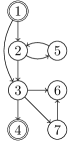
It turns out quite intuitively that some update schedules will lead to the same dynamics, when the ordered partitions are very close and the difference relies on components far apart in the interaction digraph (see an example on Figure 1). Aracena et al. introduced in [5] the notion of update digraph to capture this fact. To an update schedule one can associate its update digraph, which is a $\{\oplus,\ominus\}$ -labeling of the arcs of the interaction digraph of the AN, such that $(i,j)$ is negative ( $\ominus$ ) when $i$ is updated strictly before $j$ , and positive ( $\oplus$ ) otherwise. Formally, given an update schedule $B=(B_{1},\dots,B_{t})$ ,

\forall(i,j)\in A_{f}:\mathrm{lab}_{B}((i,j))=\begin{cases}\oplus&\text{if }i\in B_{t_{i}}\text{ and }j\in B_{t_{j}}\text{ with }t_{i}\geq t_{j},\\ \ominus&\text{if }i\in B_{t_{i}}\text{ and }j\in B_{t_{j}}\text{ with }t_{i}<t_{j}.\end{cases}

Remark 1.

Loops are always labeled $\oplus$ , hence we consider all interaction digraphs loopless.

The following result has been established: given two update schedules, if the relative order of updates among all adjacent components are identical, then the dynamics are identical.

Theorem 2 ([5]).

Given an AN $f$ and two update schedules $B,B^{\prime}$ , if $\mathrm{lab}_{B}=\mathrm{lab}_{B^{\prime}}$ then $f^{(B)}=f^{(B^{\prime})}$ .

This leads naturally to an equivalence relation on update schedules, at the heart of the present work.

Definition 3.

$B\equiv B^{\prime}$ if and only if $\mathrm{lab}_{B}=\mathrm{lab}_{B^{\prime}}$ .

It is very important to note that, though every update schedule corresponds to a $\{\oplus,\ominus\}$ -labeling of $G_{f}$ , the reciprocal of this fact is not true. For example, a cycle with all arcs labeled $\ominus$ would lead to a contradiction where components are updated strictly before themselves. Aracena et al. gave a precise characterization of valid update digraphs (i.e. the ones corresponding to at least one update schedule).

Theorem 4 ([4]).

A labeling function $\mathrm{lab}:A\to\{\oplus,\ominus\}$ is valid if and only if there is no cycle $(i_{0},i_{1},\dots,i_{k})$ , with $i_{0}=i_{k}$ , of length $k>0$ such that both:

•

$\forall\leavevmode\nobreak\ 0\leq j<k:((i_{j},i_{j+1})\in A\wedge\mathrm{lab}((i_{j},i_{j+1}))=\oplus)\vee((i_{j+1},i_{j})\in A\wedge\mathrm{lab}((i_{j+1},i_{j}))=\ominus)$ ,
•

$\exists\leavevmode\nobreak\ 0\leq j<k:\mathrm{lab}((i_{j+1},i_{j}))=\ominus$ .

In words, the multidigraph where the labeling is unchanged but the orientation of negative arcs is reversed, does not contain a cycle with at least one negative arc (forbidden cycle).

As a corollary, one can decide in polynomial time whether a labeling is valid.
Valid Update Digraph Problem (Valid-UD Problem)
Input: a labeling $\mathrm{lab}:A\to\{\oplus,\ominus\}$ of a digraph $G=(V,A)$ . Question: is $\mathrm{lab}$ valid?

Corollary 5 ([4]).

Valid-UD Problem is in $\mathsf{P}$ .

We are interested in the following counting problem.
Update Digraphs Counting (#UD)
Input: a digraph $G=(V,A)$ . Output: $\#\texttt{UD}(G)=|\{\mathrm{lab}:A\to\{\ominus,\oplus\}\mid\mathrm{lab}\text{ is valid}\}|$ .

The following definition is motivated by Theorem 4.

Definition 6.

Given a directed graph $G=(V,A)$ , let $\bar{G}=(V,\bar{A})$ denote the undirected multigraph underlying $G$ , i.e. with an edge $\{i,j\}\in\bar{A}$ for each $(i,j)\in A$ .

Remark 7.

We can restrict our study to connected digraphs (that is, such that $\bar{G}$ is connected), because according to Theorem 4 the only invalid labelings contain (forbidden) cycles. Given some $G$ with $V_{1},\dots,V_{k}$ its connected components, and $G[V_{i}]$ the subdigraph induced by $V_{i}$ , we straightforwardly have

\#\texttt{UD}(G)=\prod_{i\in[k]}\#\texttt{UD}(G[V_{i}]),

and this decomposition can be computed in linear time from folklore algorithms.

Theorem 8.

#UD is in $\mathsf{\#P}$ .

Proof.

The following non-deterministic algorithm runs in polynomial time (step 2 from Corollary 5), and its number of accepting branches equals $\#\texttt{UD}(G)$ :

1.

guess a labeling $\mathrm{lab}:A\to\{\oplus,\ominus\}$ (polynomial space),
2.

accept if $\mathrm{lab}$ is valid, otherwise reject.

∎

3 Further known results

The consideration of update digraphs has been initiated by Aracena et al. in 2009 [5], with their characterization (Theorem 4) in [4]. In Section 4 we will present a problem closely related to #UD that has been proven to be $\mathsf{NP}$ -complete in [4], UD Problem, and bounds that we can deduce on #UD (Corollary 10, from [3]). In [2] the authors present an algorithm to enumerate update digraphs, and prove its correctness. They also consider a surprisingly complex question: given an AN $f$ , knowing whether there exist two block-sequential update schedules $B,B^{\prime}$ such that $f^{(B)}\neq f^{(B^{\prime})}$ , is $\mathsf{NP}$ -complete. The value of $\#\texttt{UD}(G)$ is known to be $3^{n}-2^{n+1}+2$ for bidirected cycles on $n$ vertices [31], and to equal $n!$ if and only if the digraph is a tournament on $n$ vertices [3].

4 Counting update digraphs is $\mathsf{\#P}$ -complete

The authors of [4] have exhibited an insightful relation between valid labelings and feedback arc sets of a digraph. We recall that a feedback arc set (FAS) of $G=(V,A)$ is a subset of arcs $F\subseteq A$ such that the digraph $(V,A\setminus F)$ is acyclic, and its size is $|F|$ . This relation is developed inside the proof of $\mathsf{NP}$ -completeness of the following decision problem. We reproduce it as a Lemma, with its argumentation for the sake of comprehension.
Update Digraph Problem (UD Problem)
Input: a digraph $G=(V,A)$ and an integer $k$ . Question: does there exist a valid labeling of size at most $k$ ?
The size of a labeling is its number of $\oplus$ labels. It is clear that minimizing the number of $\oplus$ labels (or equivalently maximizing the number of $\ominus$ labels) is the difficult direction, the contrary being easy because $\mathrm{lab}(a)=\oplus$ for all $a\in A$ is always valid (and corresponds to the parallel update schedule $B^{\texttt{par}}$ ).

Lemma 9 (appears in [4, Theorem 16]).

There exists a bijection between minimal valid labelings and minimal feedback arc sets of a digraph $G=(V,A)$ .

Proof.

To get the bijection, we simply identify a labeling $\mathrm{lab}$ with its set of arcs labeled $\oplus$ , denoted $F_{\mathrm{lab}}=\{a\in A\mid\mathrm{lab}(a)=\oplus\}$ .

Given any valid labeling $\mathrm{lab}$ , $F_{\mathrm{lab}}$ is a FAS, otherwise there is a cycle with all its arcs label $\ominus$ , which is forbidden.

Given a minimal FAS $F$ , let us now argue that $\mathrm{lab}$ such that $F_{\mathrm{lab}}=F$ is a valid labeling. First observe that for every $a\in F$ there is a cycle in $G$ containing $a$ and no other arc of $F$ , otherwise $F$ would not be minimal (removing an arc $a$ not fulfilling this observation would give a smaller FAS). By contradiction, if $\mathrm{lab}$ creates a forbidden cycle $C$ , then to every arc $a$ labeled $\oplus$ in $C$ we can associate, from the previous observation, a cycle $C_{a}$ containing no other arc labeled $\oplus$ and distinct from $C$ . It follows that replacing all such arcs $a$ in $C$ with $C_{a}\setminus\{a\}$ gives a cycle which now contains only arcs labeled $\ominus$ , i.e. a cycle (recall that the orientation of $\ominus$ arcs is reversed in forbidden cycles) with no arc in $F$ , a contradiction. ∎

Any valid labeling corresponds to a FAS, and every minimal FAS corresponds to a valid labeling, hence the following bounds hold. The strict inequality for the lower bound comes from the fact that labeling all arcs $\oplus$ does not give a minimal FAS, as noted in [3] where the authors also consider the relation between update digraphs (valid labelings) and feedback arc sets, but from another perspective.

Corollary 10 ([4]).

For any digraph $G$ , let $\#\texttt{FAS}(G)$ and $\#\texttt{MFAS}(G)$ be respectively the number of FAS and minimal FAS of $G$ , then $\#\texttt{MFAS}(G)<\#\texttt{UD}(G)\leq\#\texttt{FAS}(G)$ .

From Lemma 9 and results on the complexity of FAS counting problems presented in [30] (one of them coming from [37]), we have the following corollary (minimum FAS are minimal, hence the identity is a parsimonious reduction from the same problems on FAS).

Corollary 11.

Counting the number of valid labelings of minimal size is $\mathsf{\#P}$ -complete, and counting the number of valid labelings of minimum size is $\mathsf{\#\!\cdot\!OptP[\log n]}$ -complete.

However the correspondence given in Lemma 9 does not hold in general: there may exist some FAS $F$ such that $\mathrm{lab}$ with $F_{\mathrm{lab}}=F$ is not a valid labeling (see Figure 2 for an example). As a consequence we do not directly get a counting reduction to #UD. It nevertheless holds that #UD is $\mathsf{\#P}$ -hard, with the following reduction.

Figure 2:

F=\{(1,2),(2,3),(3,1)\}

is a FAS, but the corresponding labeling is not valid: component

3

is updated prior to

2

1

not prior to

2

, and

3

not prior to

1

, which is impossible.

Theorem 12.

#UD is $\mathsf{\#P}$ -hard.

Proof.

We present a (polynomial time) parsimonious reduction from the problem of counting the number of acyclic orientations of an undirected graph, proven to be $\mathsf{\#P}$ -hard in [26].

Given an undirected graph $G=(V,E)$ , let $\prec$ denote an arbitrary total order on $V$ . Construct the digraph $G^{\prime}=(V,A)$ with $A$ the orientation of $E$ according to $\prec$ ,

(u,v)\in A\quad\iff\quad\{u,v\}\in E\text{ and }u\prec v.

An example is given on Figure 3. A key property is that $G^{\prime}$ is acyclic, because $A$ is constructed from an order $\prec$ on $V$ (a cycle would have at least one arc $(u,v)$ with $v\prec u$ ).

We claim that there is a bijection between the valid labelings of $G^{\prime}$ and the acyclic orientations of $G$ : to a valid labeling $\mathrm{lab}:A\to\{\oplus,\ominus\}$ of $G^{\prime}$ we associate the orientation

\begin{array}[]{rr}O=&\{(u,v)\mid(u,v)\in A\text{ and }\mathrm{lab}((u,v))=\oplus\}\phantom{.}\\ &\cup\leavevmode\nobreak\ \{(v,u)\mid(u,v)\in A\text{ and }\mathrm{lab}((u,v))=\ominus\}.\end{array}

First remark that $O$ is indeed an orientation of $E$ : each edge of $E$ is transformed into an arc of $A$ , and each arc of $A$ is transformed into an arc of $O$ . An example is given on Figure 4. Now observe that $O$ is exactly obtained from $G^{\prime}$ by reversing the orientation of arcs labeled $\ominus$ by $\mathrm{lab}$ . Furthermore, a cycle in $O$ must contain at least one arc labeled $\ominus$ by $\mathrm{lab}$ , because $G^{\prime}$ is acyclic and $\oplus$ labels copy the orientation of $G^{\prime}$ . The claim therefore follows directly from the characterization of Theorem 4. ∎

5 Quasi-quadratic time algorithm for oriented cacti

The difficulty of counting the number of update digraphs comes from the interplay between various possible cycles, as is assessed by the parsimonious reduction from acyclic orientations counting problem to ${\bf\#UD}$ . Answering the problem for an oriented tree with $m$ arcs is for example very simple: all of the $2^{m}$ labelings are valid. Cactus undirected graphs are defined in terms of very restricted entanglement of cycles, which we can exploit to compute the number of update digraphs for any orientation of its edges.

Definition 13.

A cactus is a connected undirected graph such that any vertex (or equivalently any edge) belongs to at most one simple cycle (cycle without vertex repetition). An oriented cactus $G$ is a digraph such that $\bar{G}$ is a cactus.

Cacti may intuitively be thought as trees with cycles. This is indeed the idea behind the skeleton of a cactus introduced in [12], via the following notions:

•

a c-vertex is a vertex of degree two included in exactly one cycle,
•

a g-vertex is a vertex not included in any cycle,
•

remaining vertices are h-vertices,

and a graft is a maximal subtree of g- and h-vertices with no two h-vertices belonging to the same cycle. Then a cactus can be decomposed as grafts and cycles (two classes called blocks), connected at h-vertices according to a tree skeleton. These notions directly apply to oriented cacti (see an example on Figure 5).

Theorem 14.

#UD is computable in time $\mathcal{O}(n^{2}\log n\log\log n)$ for oriented cacti.

Proof.

The result is obtained from the skeleton of an oriented cactus $G$ , since potential forbidden cycles are limited to within blocks of the skeleton. From this independence, any union of valid labelings on blocks is valid, and we have the product

\#\texttt{UD}(G)=\prod_{H\in\mathcal{G}}2^{|H|}\prod_{H\in\vec{\mathcal{C}}}(2^{|H|}-1)\prod_{H\in\mathcal{C}}(2^{|H|}-2)

where $\mathcal{G}$ is the set of grafts of $G$ , $\vec{\mathcal{C}}$ is the set of cycles forming directed cycles, $\mathcal{C}$ is the set of cycles not forming directed cycles, and $|H|$ is the number of arcs in block $H$ . Indeed, grafts cannot create forbidden cycles hence any $\{\oplus,\ominus\}$ -labeling will be valid, cycles forming a directed cycle can create exactly one forbidden cycle (with $\ominus$ labels on all arcs), and cycles not forming a directed cycle can create exactly two forbidden cycles (one for each possible direction of the cycle). In a first step the skeleton of a cactus can be computed in linear time [12]. Then, since the size $n$ of the input is equal (up to a constant) to the number of arcs, the size of the output contains $\mathcal{O}(n)$ bits (upper bounded by the number of $\{\oplus,\ominus\}$ -labelings), thus naively we have $\mathcal{O}(n)$ terms, each of $\mathcal{O}(n)$ bits, and the $\mathcal{O}(n\log n\log\log n)$ Schönhage–Strassen integer multiplication algorithm [36] gives the result. ∎

Remark 15.

Assuming multiplications to be done in constant time in the above result would be misleading, because we are multiplying integers having a number of digits in the magnitude of the input size. Also, the result may be slightly strengthened by considering the $\mathcal{O}(n\log n\leavevmode\nobreak\ 2^{2\log^{*}n})$ algorithm by Fürer in 2007 [18], and maybe more efficient integer multiplication algorithms in the future, such as the $\mathcal{O}(n\log n)$ algorithm recently claimed [20].

6 Series-parallel decomposition method

In this section we present a divide and conquer method in order to solve #UD, i.e. in order to count the number of valid labelings (update digraphs) of a given digraph. What will be essential in this decomposition method is not the orientation of arcs, but rather the topology of the underlying undirected (multi)graph $\bar{G}$ . The (de)composition is based on defining two endpoints on our digraphs, and composing them at their endpoints. It turns out to be closely related to series-parallel graphs first formalized to model electric networks in 1892 [27]. In Subsection 6.1 we present the operations of composition, and in Subsection 6.2 we show how it applies to the family of oriented series-parallel graphs.

6.1 Sequential, parallel, and free compositions

Let us first introduce some notations and terminology on the characterization of valid labelings provided by Theorem 4. Given $\mathrm{lab}:A\to\{\oplus,\ominus\}$ , we denote $\tilde{G}_{\mathrm{lab}}=(V,\tilde{A})$ the multidigraph obtained by reversing the orientation of negative arcs:

(i,j)\in\tilde{A}\quad\iff\quad\begin{array}[]{r}(i,j)\in A\text{ and }\mathrm{lab}((i,j))=\oplus,\\ \text{or }(j,i)\in A\text{ and }\mathrm{lab}((j,i))=\ominus.\end{array}

For simplicity we abuse the notation and still denote $\mathrm{lab}$ the labeling of the arcs of $\tilde{G}_{\mathrm{lab}}$ (arcs keep their label from $G$ to $\tilde{G}_{\mathrm{lab}}$ ). From Theorem 4, $\mathrm{lab}$ is a valid labeling if and only if $\tilde{G}_{\mathrm{lab}}$ does not contain any cycle with at least one arc labeled $\ominus$ , called forbidden cycle (it may contain cycles with all arcs labeled $\oplus$ ). A path from $i$ to $j$ in $\tilde{G}_{\mathrm{lab}}$ is called negative if it contains at least one arc labeled $\ominus$ , and positive otherwise.

Definition 16.

A source-sink labeled graph (ss-graph) $(G,\alpha,\beta)$ is a multigraph $G$ with two distinguished vertices $\alpha\neq\beta$ . A triple $(G,\alpha,\beta)$ with $G$ a digraph such that $(\bar{G},\alpha,\beta)$ is a ss-graph, is called an oriented ss-graph (oss-graph).

We can decompose the set of update digraphs (denoted $\texttt{UD}(G)=\{\mathrm{lab}:A\to\{\oplus,\ominus\}\mid\mathrm{lab}\text{ is valid}\}$ ) into an oss-graph $(G,\alpha,\beta)$ , based on the follow sets.

\begin{array}[]{rl}\texttt{UD}(G)_{\alpha\to\beta}^{+}=\{\mathrm{lab}\in\texttt{UD}(G)\mid&\text{there {\bf exists} a path from }\alpha\text{ to }\beta\text{ in }\tilde{G}_{\mathrm{lab}},\\ &\text{and {\bf all} paths from }\alpha\text{ to }\beta\text{ in }\tilde{G}_{\mathrm{lab}}\text{ are {\bf positive}}\}\\[5.0pt] \texttt{UD}(G)_{\alpha\to\beta}^{-}=\{\mathrm{lab}\in\texttt{UD}(G)\mid&\text{there {\bf exists} a {\bf negative} path from }\alpha\text{ to }\beta\text{ in }\tilde{G}_{\mathrm{lab}}\}\\[5.0pt] \texttt{UD}(G)_{\alpha\to\beta}^{\varnothing}=\{\mathrm{lab}\in\texttt{UD}(G)\mid&\text{there exist {\bf no path} from }\alpha\text{ to }\beta\text{ in }\tilde{G}_{\mathrm{lab}}\}\end{array}

We define analogously $\texttt{UD}(G)_{\beta\to\alpha}^{+}$ , $\texttt{UD}(G)_{\beta\to\alpha}^{-}$ , $\texttt{UD}(G)_{\beta\to\alpha}^{\varnothing}$ , and partition $\texttt{UD}(G)$ as:

1.

$\texttt{UD}(G)_{\alpha,\beta}^{+,+}=\texttt{UD}(G)_{\alpha\to\beta}^{+}\cap\texttt{UD}(G)_{\beta\to\alpha}^{+}$
2.

$\texttt{UD}(G)_{\alpha,\beta}^{+,\varnothing}=\texttt{UD}(G)_{\alpha\to\beta}^{+}\cap\texttt{UD}(G)_{\beta\to\alpha}^{\varnothing}$
3.

$\texttt{UD}(G)_{\alpha,\beta}^{-,\varnothing}=\texttt{UD}(G)_{\alpha\to\beta}^{-}\cap\texttt{UD}(G)_{\beta\to\alpha}^{\varnothing}$
4.

$\texttt{UD}(G)_{\alpha,\beta}^{\varnothing,+}=\texttt{UD}(G)_{\alpha\to\beta}^{\varnothing}\cap\texttt{UD}(G)_{\beta\to\alpha}^{+}$
5.

$\texttt{UD}(G)_{\alpha,\beta}^{\varnothing,-}=\texttt{UD}(G)_{\alpha\to\beta}^{\varnothing}\cap\texttt{UD}(G)_{\beta\to\alpha}^{-}$
6.

$\texttt{UD}(G)_{\alpha,\beta}^{\varnothing,\varnothing}=\texttt{UD}(G)_{\alpha\to\beta}^{\varnothing}\cap\texttt{UD}(G)_{\beta\to\alpha}^{\varnothing}$

Notice that the three missing combinations, $\texttt{UD}(G)_{\alpha,\beta}^{+,-}$ , $\texttt{UD}(G)_{\alpha,\beta}^{-,+}$ and $\texttt{UD}(G)_{\alpha,\beta}^{-,-}$ , would always be empty because such labelings contain a forbidden cycle. For convenience let us denote $S=\{(+,+),(+,\varnothing),(-,\varnothing),(\varnothing,+),(\varnothing,-),(\varnothing,\varnothing)\}$ . Given any oss-graph $(G,\alpha,\beta)$ we have

\displaystyle\#\texttt{UD}(G)=\sum_{(s,t)\in S}\#\texttt{UD}(G)_{\alpha,\beta}^{s,t}

(1)

where $\#\texttt{UD}(G)_{\alpha,\beta}^{s,t}=|\texttt{UD}(G)_{\alpha,\beta}^{s,t}|$ . Oss-graphs may be thought as black boxes, we will compose them using the values of $\#\texttt{UD}(G)_{\alpha,\beta}^{s,t}$ , regardless of their inner topologies.

Definition 17.

We define three types of compositions (see Figure 6).

•

The series composition of two oss-graphs $(G,\alpha,\beta)$ and $(G^{\prime},\alpha^{\prime},\beta^{\prime})$ with $V\cap V^{\prime}=\emptyset$ , is the oss-graph $\mathcal{S}((G,\alpha,\beta),(G^{\prime},\alpha^{\prime},\beta^{\prime}))=(D,\alpha,\beta^{\prime})$ with $D$ the one-point join of $G$ and $G^{\prime}$ identifying components $\beta,\alpha^{\prime}$ as one single component.
•

The parallel composition of two oss-graphs $(G,\alpha,\beta)$ and $(G^{\prime},\alpha^{\prime},\beta^{\prime})$ with $V\cap V^{\prime}=\emptyset$ , is the oss-graph $\mathcal{P}((G,\alpha,\beta),(G^{\prime},\alpha^{\prime},\beta^{\prime}))=(D,\alpha,\beta)$ with $D$ the two-points join of $G$ and $G^{\prime}$ identifying components $\alpha,\alpha^{\prime}$ and $\beta,\beta^{\prime}$ as two single components.
•

The free composition at $v,v^{\prime}$ of an oss-graph $(G=(V,A),\alpha,\beta)$ and a digraph $G^{\prime}=(V^{\prime},A^{\prime})$ with $V\cap V^{\prime}=\emptyset$ , $v\in V$ , $v^{\prime}\in V^{\prime}$ , is the oss-graph $\mathcal{F}((G,\alpha,\beta),G^{\prime})=(D,\alpha,\beta)$ with $D$ the one-point join of $G$ and $G^{\prime}$ identifying $v,v^{\prime}$ as one single component.

Remark that the three types of compositions from Definition 17 also apply to (undirected) ss-graph $(\bar{G},\alpha,\beta)$ . Series and free compositions differ on the endpoints of the obtained oss-graph, which has important consequences on counting the number of update digraphs, as stated in the following results. We will see in Theorem 23 from Subsection 6.2 that both series and free compositions are needed in order to decompose the family of (general) oriented series-parallel graphs (to be defined).

Figure 6: Example of series and parallel compositions, and a free composition at

u,\beta^{\prime}

Lemma 18.

For $(D,\alpha,\beta^{\prime})=\mathcal{S}((G,\alpha,\beta),(G^{\prime},\alpha^{\prime},\beta^{\prime}))$ , the values of $\#\texttt{UD}(D)_{\alpha,\beta^{\prime}}^{s,t}$ for all $(s,t)\in S$ can be computed in time $\mathcal{O}(n\log n\log\log n)$ (with $n$ the binary length of the values) from the values of $\#\texttt{UD}(G)_{\alpha,\beta}^{s,t}$ and $\#\texttt{UD}(G^{\prime})_{\alpha^{\prime},\beta^{\prime}}^{s,t}$ for all $(s,t)\in S$ .

Proof.

The result is obtained by considering the $36$ couples of some $\texttt{UD}(G)_{\alpha,\beta}^{s,t}$ with $(s,t)\in S$ and some $\texttt{UD}(G^{\prime})_{\alpha^{\prime},\beta^{\prime}}^{s^{\prime},t^{\prime}}$ with $(s^{\prime},t^{\prime})$ . For example, when we take the union of any labeling $\mathrm{lab}$ in $\texttt{UD}(G)_{\alpha,\beta}^{+,\varnothing}$ (in $\tilde{G}_{\mathrm{lab}}$ there is at least one path from $\alpha$ to $\beta$ , all paths from $\alpha$ to $\beta$ positive, and no path from $\beta$ to $\alpha$ ) and any labeling $\mathrm{lab}^{\prime}$ in $\texttt{UD}(G^{\prime})_{\alpha^{\prime},\beta^{\prime}}^{-,\varnothing}$ (in $\tilde{G^{\prime}}_{\mathrm{lab}^{\prime}}$ there is a negative path from $\alpha^{\prime}$ to $\beta^{\prime}$ , and no path from $\beta^{\prime}$ to $\alpha^{\prime}$ ), we obtain a valid labeling of $D$ with at least one negative path from $\alpha$ to $\beta^{\prime}$ , and no path from $\beta^{\prime}$ to $\alpha$ , hence an element of $\texttt{UD}(D)_{\alpha,\beta^{\prime}}^{-,\varnothing}$ . We can deduce that $\texttt{UD}(D)_{\alpha,\beta^{\prime}}^{-,\varnothing}$ contains these $\#\texttt{UD}(G)_{\alpha,\beta}^{+,\varnothing}\#\texttt{UD}(G^{\prime})_{\alpha^{\prime},\beta^{\prime}}^{-,\varnothing}$ labelings. The results of this simple reasoning in all $36$ cases is presented on Table 1.

$\mathcal{S}$	$+,+$	$+,\varnothing$	$-,\varnothing$	$\varnothing,+$	$\varnothing,-$	$\varnothing,\varnothing$
$+,+$	$+,+$	$+,\varnothing$	$-,\varnothing$	$\varnothing,+$	$\varnothing,-$	$\varnothing,\varnothing$
$+,\varnothing$	$+,\varnothing$	$+,\varnothing$	$-,\varnothing$	$\varnothing,\varnothing$	$\varnothing,\varnothing$	$\varnothing,\varnothing$
$-,\varnothing$	$-,\varnothing$	$-,\varnothing$	$-,\varnothing$	$\varnothing,\varnothing$	$\varnothing,\varnothing$	$\varnothing,\varnothing$
$\varnothing,+$	$\varnothing,+$	$\varnothing,\varnothing$	$\varnothing,\varnothing$	$\varnothing,+$	$\varnothing,-$	$\varnothing,\varnothing$
$\varnothing,-$	$\varnothing,-$	$\varnothing,\varnothing$	$\varnothing,\varnothing$	$\varnothing,-$	$\varnothing,-$	$\varnothing,\varnothing$
$\varnothing,\varnothing$	$\varnothing,\varnothing$	$\varnothing,\varnothing$	$\varnothing,\varnothing$	$\varnothing,\varnothing$	$\varnothing,\varnothing$	$\varnothing,\varnothing$

Table 1: Row

(s,t)

corresponds to

\texttt{UD}(G)_{\alpha,\beta}^{s,t}

, column

(s^{\prime},t^{\prime})

corresponds to

\texttt{UD}(G^{\prime})_{\alpha^{\prime},\beta^{\prime}}^{s^{\prime},t^{\prime}}

, and cell content

(s^{\prime\prime},t^{\prime\prime})

indicates that the union of any labeling in

\texttt{UD}(G)_{\alpha,\beta}^{s,t}

and any labeling in

\texttt{UD}(G^{\prime})_{\alpha^{\prime},\beta^{\prime}}^{s^{\prime},t^{\prime}}

gives a labeling in

\texttt{UD}(D)_{\alpha,\beta^{\prime}}^{s^{\prime\prime},t^{\prime\prime}}

for

(D,\alpha,\beta^{\prime})=\mathcal{S}((G,\alpha,\beta),(G^{\prime},\alpha^{\prime},\beta^{\prime}))

This allows to compute each value $\#\texttt{UD}(D)_{\alpha,\beta^{\prime}}^{s^{\prime\prime},t^{\prime\prime}}$ as the finite sum, for each line $(s,t)$ and column $(s^{\prime},t^{\prime})$ where $(s^{\prime\prime},t^{\prime\prime})$ appears, of the term $\#\texttt{UD}(G)_{\alpha,\beta}^{s,t}\#\texttt{UD}(G^{\prime})_{\alpha^{\prime},\beta^{\prime}}^{s^{\prime},t^{\prime}}$ . As an example we have $\#\texttt{UD}(D)_{\alpha,\beta^{\prime}}^{+,\varnothing}=\#\texttt{UD}(G)_{\alpha,\beta}^{+,+}\#\texttt{UD}(G^{\prime})_{\alpha^{\prime},\beta^{\prime}}^{+,\varnothing}+\#\texttt{UD}(G)_{\alpha,\beta}^{+,\varnothing}\#\texttt{UD}(G^{\prime})_{\alpha^{\prime},\beta^{\prime}}^{+,+}+\#\texttt{UD}(G)_{\alpha,\beta}^{+,\varnothing}\#\texttt{UD}(G^{\prime})_{\alpha^{\prime},\beta^{\prime}}^{+,\varnothing}$ . Summations on $n$ bits are performed in linear time with schoolbook algorithm, and multiplications on $n$ bits are performed in time $\mathcal{O}(n\log n\log\log n)$ from Schönhage–Strassen algorithm [36]. ∎

Lemma 19.

For $(D,\alpha,\beta)=\mathcal{P}((G,\alpha,\beta),(G^{\prime},\alpha^{\prime},\beta^{\prime}))$ , the values of $\#\texttt{UD}(D)_{\alpha,\beta}^{s,t}$ for all $(s,t)\in S$ can be computed in time $\mathcal{O}(n\log n\log\log n)$ (with $n$ the binary length of the values) from the values of $\#\texttt{UD}(G)_{\alpha,\beta}^{s,t}$ and $\#\texttt{UD}(G^{\prime})_{\alpha^{\prime},\beta^{\prime}}^{s,t}$ for all $(s,t)\in S$ .

Proof.

The proof is analogous to Lemma 18, with Table 2. Remark that in this case, it is possible to create invalid labelings for $D$ (containing some forbidden cycle) from the union of two valid labelings for $G$ and $G^{\prime}$ . For example, when we take the union of any labeling $\mathrm{lab}$ in $\texttt{UD}(G)_{\alpha,\beta}^{+,+}$ (in $\tilde{G}_{\mathrm{lab}}$ there is at least one path from $\alpha$ to $\beta$ , all paths from $\alpha$ to $\beta$ positive, and the same from $\beta$ to $\alpha$ ) and any labeling $\mathrm{lab}^{\prime}$ in $\texttt{UD}(G^{\prime})_{\alpha^{\prime},\beta^{\prime}}^{-,\varnothing}$ (in $\tilde{G^{\prime}}_{\mathrm{lab}^{\prime}}$ there is a negative path from $\alpha^{\prime}$ to $\beta^{\prime}$ , and no path from $\beta^{\prime}$ to $\alpha^{\prime}$ ), we obtain an invalid labeling of $D$ because the concatenation of a positive path from $\alpha$ to $\beta$ with a negative path from $\beta^{\prime}$ to $\alpha^{\prime}$ gives a forbidden cycle in $D$ (recall that $\alpha,\alpha^{\prime}$ and $\beta,\beta^{\prime}$ are identified).

$\mathcal{P}$	$+,+$	$+,\varnothing$	$-,\varnothing$	$\varnothing,+$	$\varnothing,-$	$\varnothing,\varnothing$
$+,+$	$+,+$	$+,+$		$+,+$		$+,+$
$+,\varnothing$	$+,+$	$+,\varnothing$	$-,\varnothing$	$+,+$		$+,\varnothing$
$-,\varnothing$		$-,\varnothing$	$-,\varnothing$			$-,\varnothing$
$\varnothing,+$	$+,+$	$+,+$		$\varnothing,+$	$\varnothing,-$	$\varnothing,+$
$\varnothing,-$				$\varnothing,-$	$\varnothing,-$	$\varnothing,-$
$\varnothing,\varnothing$	$+,+$	$+,\varnothing$	$-,\varnothing$	$\varnothing,+$	$\varnothing,-$	$\varnothing,\varnothing$

Table 2: Row

(s,t)

corresponds to

\texttt{UD}(G)_{\alpha,\beta}^{s,t}

, column

(s^{\prime},t^{\prime})

corresponds to

\texttt{UD}(G^{\prime})_{\alpha^{\prime},\beta^{\prime}}^{s^{\prime},t^{\prime}}

, and cell content

(s^{\prime\prime},t^{\prime\prime})

indicates that the union of any labeling in

\texttt{UD}(G)_{\alpha,\beta}^{s,t}

and any labeling in

\texttt{UD}(G^{\prime})_{\alpha^{\prime},\beta^{\prime}}^{s^{\prime},t^{\prime}}

gives a labeling in

\texttt{UD}(D)_{\alpha,\beta}^{s^{\prime\prime},t^{\prime\prime}}

for

(D,\alpha,\beta)=\mathcal{P}((G,\alpha,\beta),(G^{\prime},\alpha^{\prime},\beta^{\prime}))

. Empty cells mean that unions give invalid labelings.

∎

Note that Remark 15 also applies to Lemmas 18 and 19. For the free composition the count is easier.

Lemma 20.

For $(D,\alpha,\beta)=\mathcal{F}((G,\alpha,\beta),G^{\prime})$ , we have $\#\texttt{UD}(D)_{\alpha,\beta}^{s,t}=\#\texttt{UD}(G)_{\alpha,\beta}^{s,t}\#\texttt{UD}(G^{\prime})$ for all $(s,t)\in S$ .

Proof.

The endpoints of the oss-graph $(D,\alpha,\beta)$ are the endpoints of the oss-graph $(G,\alpha,\beta)$ , and it is not possible to create a forbidden cycle in the union of a valid labeling on $G$ and a valid labeling of $G^{\prime}$ , therefore the union is always a valid labeling of $D$ , each one belonging to the part $(s,t)$ of $(D,\alpha,\beta)$ corresponding to the part $(s,t)\in S$ of $(G,\alpha,\beta)$ . ∎

6.2 Application to oriented series-parallel graphs

The series and parallel compositions of Definition 17 correspond exactly to the class of two-terminal series-parallel graphs from [1, 33, 39].

Definition 21.

A ss-graph $(G,\alpha,\beta)$ is two-terminal series-parallel (a ttsp-graph) if and only if one the following holds.

•

$(G,\alpha,\beta)$ is a base ss-graph with two vertices $\alpha,\beta$ and one edge $\{\alpha,\beta\}$ .
•

$(G,\alpha,\beta)$ is obtained by a series or parallel composition¹¹1With Definition 17 applied to (undirected) ss-graphs. of two ttsp-graphs.

In this case $G$ alone is called a blind ttsp-graph.

Adding the free composition allows to go from two-terminal series-parallel graphs to (general) series-parallel graphs [15, 39]. More precisely, it allows exactly to add tree structures to ttsp-graphs, as we argue now (ttsp-graphs do not contain arbitrary trees, its only acyclic graphs being simple paths; e.g. one cannot build a claw from Definition 21).

Definition 22.

A multigraph $G$ is series-parallel (sp-graph) if and only if all its 2-connected components are blind ttsp-graphs. A digraph $G$ such that $\bar{G}$ is an sp-graph, is called an oriented sp-graph (osp-graph).

The family of sp-graphs corresponds to the multigraphs obtained by series, parallel and free compositions from base ss-graphs. See Figure 7 for an example $G$ of osp-graph illustrating Theorem 23, and the decomposition method to compute $\#\texttt{UD}(G)$ (Theorem 24).

Theorem 23.

$G$ is an sp-graph if and only if $(G,\alpha,\beta)$ is obtained by series, parallel and free compositions from base ss-graphs, for some $\alpha,\beta$ .

Proof sketch (see Appendix A).

Free compositions allow to build all sp-graphs, because it offers the possibility to create the missing tree structures of ttsp-graphs: arbitrary 1-connected components linking 2-connected ttsp-graphs. Moreover free compositions do not go beyond sp-graphs, since the obtained multigraphs still have treewidth 2. ∎

Theorem 24.

#UD is solvable in time $\mathcal{O}(n^{2}\log^{2}n\log\log n)$ on osp-graphs (without promise).

Proof sketch (see Appendix A).

This is a direct consequence of Lemmas 18, 19 and 20, because all values are in $\mathcal{O}(2^{n})$ (the number of $\{\oplus,\ominus\}$ -labelings) hence on $\mathcal{O}(n)$ bits, the values of $\#\texttt{UD}(G)_{\alpha,\beta}^{s,t}$ are trivial for oriented base ss-graphs, and we perform $\mathcal{O}(n\log n)$ compositions (to reach Formula 1). The absence of promise comes from a linear time recognition algorithm in [39] for ttsp-graphs, which also provides the decomposition structure. ∎

Again, Remark 15 applies to Theorem 24.

7 Conclusion

Our main result is the $\mathsf{\#P}$ -completeness of #UD, i.e. of counting the number of non-equivalent block-sequential update schedules of a given AN $f$ . We proved that this count can nevertheless be done in $\mathcal{O}(n^{2}\log n\log\log n)$ time for oriented cacti, and in $\mathcal{O}(n^{2}\log^{2}n\log\log n)$ time for oriented series-parallel graphs. This last result has been obtained via a decomposition method providing a divide-and-conquer algorithm.

Remark that cliques or tournaments are intuitively difficult instances of #UD, because of the intertwined structure of potential forbidden cycles. It turns out that $K_{4}$ is the smallest clique that cannot be build with series, parallel and free decompositions, and that series-parallel graphs (Definition 22) correspond exactly to the family of $K_{4}$ -minor-free graphs [15] (it is indeed closed by minor [35]). In further works we would like to extend this caracterization and the decomposition method to (di)graphs with multiple endpoints.

The complexity analysis of the algorithms presented in Theorems 14 and 24 may be improved, and adapted to the parallel setting using the algorithms presented in [9, 23]. One may also ask for which other classes of digraphs is $\#\texttt{UD}(G)$ computable efficiently (in polynomial time)? Since we found such an algorithm for graphs of treewidth 2, could it be that the problem is fixed parameter tractable on bounded treewidth digraphs? Rephrased more directly, could a general tree decomposition (which, according to the proof of Theorem 23, is closely related to the series-parallel decomposition for treewidth 2) be exploited to compute the solution to #UD? Alternatively, what other types of decompositions one can consider in order to ease the computation of $\#\texttt{UD}(G)$ ?

Finally, from the multiplication obtained for one-point join of two graphs (Lemma 20 on free composition), we may ask whether $\#\texttt{UD}(G)$ is an evaluation of the Tutte polynomial? From its universality [11], it remains to know whether there is a deletion-contradiction reduction. However defining a Tutte polynomial for directed graphs is still an active area of research [7, 13, 32, 42].

Acknowledgments

This work was mainly funded by our salaries as French agents (affiliated to Laboratoire Cogitamus (CN), Aix-Marseille Univ, Univ. de Toulon, CNRS, LIS, UMR 7020, Marseille, France (KP, SS and LV), Univ. Côte d’Azur, CNRS, I3S, UMR 7271, Sophia Antipolis, France (KP), and École normale supérieure de Lyon, Computer Science department, Lyon, France (LV)), and secondarily by the projects ANR-18-CE40-0002 FANs, ECOS-CONICYT C16E01, STIC AmSud 19-STIC-03 (Campus France 43478PD).

References

[1] A. Ádám. On graphs in which two vertices are distinguished. Acta Mathematica Academiae Scientiarum Hungaricae, 12:377–397, 1964.
[2] J. Aracena, J. Demongeot, É. Fanchon, and M. Montalva. On the number of different dynamics in Boolean networks with deterministic update schedules. Mathematical Biosciences, 242:188–194, 2013.
[3] J. Aracena, J. Demongeot, É. Fanchon, and M. Montalva. On the number of update digraphs and its relation with the feedback arc sets and tournaments. Discrete Applied Mathematics, 161:1345–1355, 2013.
[4] J. Aracena, É. Fanchon, M. Montalva, and M. Noual. Combinatorics on update digraphs in Boolean networks. Discrete Applied Mathematics, 159:401–409, 2011.
[5] J. Aracena, E. Goles, A. Moreira, and L. Salinas. On the robustness of update schedules in Boolean networks. Biosystems, 97:1–8, 2009.
[6] J. Aracena, L. Gómez, and L. Salinas. Limit cycles and update digraphs in Boolean networks. Discrete Applied Mathematics, 161:1–12, 2013.
[7] J. Awan and O. Bernardi. Tutte polynomials for directed graphs. Journal of Combinatorial Theory, Series B, 140:192–247, 2020.
[8] H. L. Bodlaender. A partial k-arboretum of graphs with bounded treewidth. Theoretical Computer Science, 209(1):1–45, 1998.
[9] H. L. Bodlaender and B. de Fluiter. Parallel algorithms for series parallel graphs. In Proceedings of ESA’96, volume 1136 of LNCS, pages 277–289, 1996.
[10] F. Bridoux, C. Gaze-Maillot, K. Perrot, and S. Sené. Complexity of limit-cycle problems in Boolean networks. arXiv:2001.07391, 2020.
[11] T. H. Brylawski. A decomposition for combinatorial geometries. Transactions of the American Mathematical Society, 171:235–282, 1972.
[12] R. E. Burkard and J. Krarup. A linear algorithm for the pos/neg-weighted 1-median problem on a cactus. Computing, 60:193–215, 1998.
[13] S. H. Chan. Abelian sandpile model and Biggs-Merino polynomial for directed graphs. Journal of Combinatorial Theory, Series A, 154:145–171, 2018.
[14] B. de Fluiter. Algorithms for graphs of small treewidth. PhD thesis, University of Utrecht, 1997.
[15] R. J. Duffin. Topology of series-parallel networks. Journal of Mathematical Analysis and Applications, 10:303–318, 1965.
[16] B. Elspas. The theory of autonomous linear sequential networks. IRE Trans. Circuit Theory, 6:45–60, 1959.
[17] N. Fatès. A guided tour of asynchronous cellular automata. Journal of Cellular Automata, 9:387–416, 2014.
[18] M. Fürer. Faster Integer Multiplication. In Proceedings of STOC’07, pages 57–66, 2007.
[19] E. Goles, D. Maldonado, P. Montealegre, and M. Ríos-Wilson. On the complexity of asynchronous freezing cellular automata. arXiv:1910.10882, 2019.
[20] D. Harvey and J. Van Der Hoeven. Integer multiplication in time O(n log n). HAL:hal-02070778, 2019.
[21] J. Hopcroft and R. Tarjan. Algorithm 447: efficient algorithms for graph manipulation. Communications of the ACM, 16:372–378, 1973.
[22] D. A. Huffman. Canonical forms for information-lossless finite-state logical machines. IRE Trans. Inform. Theory, 5:41–59, 1959.
[23] J. Jájá. An introduction to parallel algorithms. Addison-Wesley, 1992.
[24] S. A. Kauffman. Homeostasis and differentiation in random genetic control networks. Nature, 224:177–178, 1969.
[25] S. C. Kleene. Representation of events in nerve nets and finite automata. Project RAND RM–704, US Air Force, 1951.
[26] N. Linial. Hard enumeration problems in geometry and combinatorics. SIAM Journal on Algebraic Discrete Methods, 7:331–335, 1986.
[27] P. A. MacMahon. The combinations of resistances. The Electrician, 28:601–602, 1892.
[28] W. S. McCulloch and W. Pitts. A logical calculus of the ideas immanent in nervous activity. Journal of Mathematical Biophysics, 5:115–133, 1943.
[29] M. Noual and S. Sené. Synchronism versus asynchronism in monotonic Boolean automata networks. Natural Computing, 17:393–402, 2018.
[30] K. Perrot. On the complexity of counting feedback arc sets. arXiv:1909.03339, 2019.
[31] K. Perrot, M. Montalva-Medel, P. P. B. de Oliveira, and E. L. P. Ruivo. Maximum sensitivity to update schedule of elementary cellular automata over periodic configurations. Natural Computing, 19:51–90, 2020.
[32] K. Perrot and V. T. Pham. Chip-firing game and partial Tutte polynomial for Eulerian digraphs. Electronic Journal of Combinatorics, 23(1), 2016.
[33] J. Riordan and C. E. Shannon. The number of two-terminal series-parallel networks. Journal of Mathematics and Physics, 21:83–93, 1942.
[34] F. Robert. Blocs-H-matrices et convergence des méthodes itératives classiques par blocs. Linear Algebra and its Applications, 2:223–265, 1969.
[35] N. Robertson and P. D. Seymour. Graph Minors. XX. Wagner’s conjecture. Journal of Combinatorial Theory, Series B, 92:325–357, 2004.
[36] A. Schönhage and V. Strassen. Schnelle Multiplikation großer Zahlen. Computing, 7:281–292, 1971.
[37] B. Schwikowski and E. Speckenmeyer. On enumerating all minimal solutions of feedback problems. Discrete Applied Mathematics, 117:253–265, 2002.
[38] R. Thomas. Boolean formalization of genetic control circuits. Journal of Theoretical Biology, 42:563–585, 1973.
[39] J. Valdes, R. E. Tarjan, and E. L. Lawler. The recognition of series parallel digraphs. In Proceedings of STOC’79, pages 1–12, 1979.
[40] J. Valdes Ayesta. Parsing Flowcharts and Series-Parallel Graphs. PhD thesis, Stanford University, 1978.
[41] J. A. Wald and C. J. Colbourn. Steiner trees, partial 2-trees, and minimum IFI networks. Networks, 13:159–167, 1983.
[42] K. S. Yow. Tutte-Whitney polynomials for directed graphs and maps. PhD thesis, Monash University, 2019.

Appendix A Full proofs for the application of the decomposition method to oriented series-parallel graphs

The concept of decomposition tree associated to ttsp-graphs, and generalized to sp-graphs, will be useful to formalize the reasonings leading to Theorems 23 and 24.

The structure of a ttsp-graph $(G=(V,E),\alpha,\beta)$ obtained from base ss-graphs by series and parallel compositions is expressed in a ttsp-tree $T_{G}=(N,F,\sigma:N\to V\times V)$ . It is a rooted binary tree, in which each node $\eta\in N$ has one of the types s-node, p-node, leaf-node, and a label $\sigma(\eta)$ consisting in a pair of vertices from $G$ . Every node $\eta\in N$ corresponds to a unique ttsp-graph $(G^{\prime},\alpha^{\prime},\beta^{\prime})$ which is a subgraph of $G$ , with $\sigma(\eta)=(\alpha^{\prime},\beta^{\prime})$ . The leaves of the tree are of type leaf-node and correspond to base ss-graphs, they are in one-to-one correspondence with the edges of $G$ . The ss-graph associated to an s-node is the series composition of its (ordered) children, and the ss-graph associated to a p-node is the parallel composition of its (unordered) children. It is worth noticing that each ttsp-graph corresponds to at least one ttsp-tree (and possibly to many ttsp-trees, even non isomorphic ones [39, Section 2.2]), and that each ttsp-tree corresponds to a unique ttsp-graph.

To this classical definition (presented for example in [39, 14]), we add f-nodes corresponding to free compositions, leading to sp-trees, as follows. The subtlety is that the two distinguished vertices of one children of a free composition are discarded. Let $(G=(V,E),\alpha,\beta)$ and $(G^{\prime}=(V^{\prime},E^{\prime}),\alpha^{\prime},\beta^{\prime})$ be the (ordered) children of an f-node $\eta$ of label $\sigma(\eta)=(v,v^{\prime})$ with $v\in V$ and $v^{\prime}\in V^{\prime}$ , the ss-graph associated to this f-node is the free composition $\mathcal{F}((G,\alpha,\beta),G^{\prime})$ (its label does not correspond to the distinguished vertices of the ss-graph). Every node $\eta\in N$ still corresponds to a unique ttsp-graph $(G^{\prime},\alpha^{\prime},\beta^{\prime})$ which is a subgraph of $G$ , with $\sigma(\eta)=(\alpha^{\prime},\beta^{\prime})$ for all but f-nodes; and for f-nodes the distinguished vertices are that of its first (left on our figures) child. We have the same correspondence between sp-graphs and sp-trees. An example is given on Figure 8.

Now remark that all free compositions may be performed at the end of the composition process, i.e. on top of the sp-tree. Indeed, free compositions can be inductively pushed towards the root of an sp-tree using the operations presented on Figure 9, which leave the sp-graph unchanged. When all free compositions are on top of an sp-tree, we say that it is in free-on-top normal form. Thus to any sp-graph corresponds at least one sp-tree in free-on-top normal form.

Proof of Theorem 23.

For the “only if” part, let $G$ be an sp-graph, with $G_{1},\dots,G_{x}$ its 2-connected components, $H_{1},\dots,H_{y}$ its remaining connected components (which are therefore trees), and $w_{1},\dots,w_{z}$ the set of vertices belonging to two 2-connected components among $G_{1},\dots,G_{x}$ . By definition $G_{1},\dots,G_{x}$ are blind ttsp-graphs, to which we can respectively associate some ttsp-trees $T_{G_{1}},\dots,T_{G_{x}}$ , which are particular cases of sp-trees. Now, take an edge $\{u,v\}$ of $H_{i}$ sharing:

•

only one vertex with some $T_{G_{j}}$ , and consider the free composition of $T_{G_{j}}$ with the base ss-graph corresponding to edge $\{u,v\}$ (joining them at that vertex), we get an sp-tree replacing $T_{G_{j}}$ ,
•

its two vertices with respectively some $T_{G_{j}}$ and $T_{G_{j^{\prime}}}$ , and consider first the free composition of $T_{G_{j}}$ with the base ss-graph corresponding to edge $\{u,v\}$ (joining them at $u$ ), this gives $T^{\prime}_{G_{j}}$ , and second the free composition of $T^{\prime}_{G_{j}}$ with $T_{G_{j^{\prime}}}$ (joining them at $v$ ), we get an sp-tree replacing both $T_{G_{j}}$ and $T_{G_{j^{\prime}}}$ ,

or take a vertex $w_{i}$ and:

•

consider the free composition of the two sp-trees to which $w_{i}$ belongs (joining them at $w_{i}$ ), we get a new sp-tree replacing them.

Repeating this process for all edges of $H_{1},\dots,H_{y}$ and all vertices $w_{1},\dots,w_{z}$ , we inductively build an sp-tree corresponding to $(G,\alpha,\beta)$ , for some $\alpha,\beta$ . Indeed, since $G$ is connected and $H_{1},\dots,H_{y}$ are only 1-connected components, all edges of $H_{1},\dots,H_{y}$ will inductively be added to the sp-trees, and from the maximality of 2-connected components $G_{1},\dots,G_{x}$ the free compositions given by $w_{i}$ always joins two sp-trees that are distinct. Consequently this process will eventually merge all ttsp-trees into a unique sp-tree corresponding to the whole ss-graph $(G,\alpha,\beta)$ (at this point $\alpha,\beta$ could be the distinguished vertices of any ttsp-tree among $T_{G_{1}},\dots,T_{G_{x}}$ , and the resulting sp-tree is in free-on-top normal form).

For the “if” part, let $(G,\alpha,\beta)$ be obtained by series, parallel and free compositions from base ss-graphs, with $T_{G}$ a corresponding sp-tree in free-on-top normal form. Thanks to the free-on-top normal form, we can adapt the tree decomposition presented in [14, Lemma 2.3.5] in order to prove that $G$ has treewidth at most 2. Let $T^{1}_{G}=(N^{1},F^{1},\sigma^{1}),\dots,T^{x}_{G}=(N^{x},F^{x},\sigma^{x})$ denote the forest of ttsp-trees excluding free compositions (but including all base ss-graphs). We construct the tree decompositions $(X^{1},T^{1}_{G}),\dots,(X^{x},T^{x}_{G})$ for the ttsp-graphs respectively corresponding to $T^{1}_{G},\dots,T^{x}_{G}$ , as follows: $X^{i}=\{X^{i}_{\eta}\mid\eta\in N^{i}\}$ and

•

for each p-node $\eta\in N^{i}$ of label $(\alpha,\beta)$ , set $X^{i}_{\eta}=\{\alpha,\beta\}$ ,
•

for each s-node $\eta\in N^{i}$ of label $(\alpha,\beta)$ and labels of its two children $(\alpha,\gamma)$ and $(\gamma,\beta)$ , set $X^{i}_{\eta}=\{\alpha,\beta,\gamma\}$ .

The tree structure of each tree decomposition is directly given by the ttsp-tree. It remains to assemble these tree decompositions according to the free compositions, in order to obtain a tree decomposition of $G$ . For each f-node of label $(v,v^{\prime})$ , i.e. identifying vertices $v,v^{\prime}$ of its children, one can simply add an edge merging two tree decompositions into a single tree decomposition, between any bag containing $v$ and any bag containing $v^{\prime}$ (and rename $v^{\prime}$ as $v$ ). The result $(X,T)$ of this process is indeed a tree decomposition of $G$ :

•

the obtained graph $T$ is a tree, as at each step two distinct trees are merged,
•

all base ss-graphs (which are leaf-nodes of $T_{G}$ ) belong to ttsp-graphs, hence all edges of $G$ are covered in some bag of the tree decompositions $(X^{1},T^{1}_{G}),\dots,(X^{x},T^{x}_{G})$ ,
•

the subtree associated to each vertex is connected, because it was connected in tree decompositions $(X^{1},T^{1}_{G}),\dots,(X^{x},T^{x}_{G})$ , and the merge of two tree decompositions connects identified vertices.

Since $(X,T)$ has bags of size at most 3, it follows that the treewidth of $G$ is at most 2. From [8, 15, 41], the family of graphs of treewidth at most 2 equals the family of sp-graphs (via the equality with $K_{4}$ -minor-free and partial 2-trees), thus $G$ is an sp-graph. ∎

Proof of Theorem 24.

Given a directed graph $G$ , one can identify in linear time the 2-connected components of $\bar{G}$ (from [21]), and check in linear time that each of them is a blind ttsp-graph (from [39, Section 2.3 and Section 3.3 for implementation details] which is based on the characterization as series-parallel reducible multigraphs from [15] and its Church-Rosser property, with the blind undirected graph oriented as in [40, Chapter 3.5]). This last algorithm also builds a ttsp-tree for each 2-connected component. In order to get an sp-tree for the whole graph, it remains to include the free compositions as in the “if” part of the proof of Theorem 23, which is also done in linear time. We are now equipped with an sp-tree (in free-on-top normal form, which is not a necessary feature) corresponding to $\bar{G}$ (in the case $G$ is an osp-graph, otherwise we reject the instance).

The second (and main) part of the algorithm is a direct application of Lemmas 18, 19 and 20. For a base ss-graph $H$ with an edge oriented as $(u,v)$ we have

\begin{array}[]{c}\#\texttt{UD}(H)_{u,v}^{+,+}=\#\texttt{UD}(H)_{u,v}^{-,\varnothing}=\#\texttt{UD}(H)_{u,v}^{\varnothing,+}=\#\texttt{UD}(H)_{u,v}^{\varnothing,\varnothing}=0\\[1.99997pt] \text{and}\quad\#\texttt{UD}(H)_{u,v}^{+,\varnothing}=\#\texttt{UD}(H)_{u,v}^{\varnothing,-}=1,\end{array}

then by induction on the structure of the sp-tree of $\bar{G}$ (which provides two distinguished vertices for the osp-graph corresponding to each node of the sp-tree) we apply Lemma 18 for s-nodes, Lemma 19 for p-nodes, and Lemma 20 for f-nodes. There are $\mathcal{O}(n\log n)$ steps with $n$ the size of the input graph, because the sp-tree has one leaf-node for each arc of $G$ and is a binary tree. Finally, all values counting some number of labelings are in $\mathcal{O}(2^{n})$ (the number of $\{\oplus,\ominus\}$ -labelings of the whole input digraph $G$ ), hence on $\mathcal{O}(n)$ bits, and the result follows. ∎

#P-completeness of counting update digraphs, cacti, and a series-parallel decomposition method

Abstract

1 Introduction

2 Definitions

Remark 1.

Theorem 2 ([5]).

Definition 3.

Theorem 4 ([4]).

Corollary 5 ([4]).

Definition 6.

Remark 7.

Theorem 8.

Proof.

3 Further known results

4 Counting update digraphs is #​𝖯\mathsf{\#P}-complete

Lemma 9 (appears in [4, Theorem 16]).

Proof.

Corollary 10 ([4]).

Corollary 11.

Theorem 12.

Proof.

5 Quasi-quadratic time algorithm for oriented cacti

Definition 13.

Theorem 14.

Proof.

Remark 15.

6 Series-parallel decomposition method

6.1 Sequential, parallel, and free compositions

Definition 16.

Definition 17.

Lemma 18.

Proof.

Lemma 19.

Proof.

Lemma 20.

Proof.

6.2 Application to oriented series-parallel graphs

Definition 21.

Definition 22.

Theorem 23.

Proof sketch (see Appendix A).

Theorem 24.

Proof sketch (see Appendix A).

7 Conclusion

Acknowledgments

References

Appendix A Full proofs for the application of the decomposition method to oriented series-parallel graphs

Proof of Theorem 23.

Proof of Theorem 24.

#P-completeness of counting update digraphs,
cacti, and a series-parallel decomposition method

4 Counting update digraphs is $\mathsf{\#P}$ -complete