OzDES multi-object fibre spectroscopy for the Dark Energy Survey: Results and second data release
Abstract
We present a description of the Australian Dark Energy Survey (OzDES) and summarise the results from its six years of operations. Using the 2dF fibre positioner and AAOmega spectrograph on the 3.9-m Anglo-Australian Telescope, OzDES has monitored 771 AGN, classified hundreds of supernovae, and obtained redshifts for thousands of galaxies that hosted a transient within the 10 deep fields of the Dark Energy Survey. We also present the second OzDES data release, containing the redshifts of almost 30,000 sources, some as faint as mag, and 375,000 individual spectra. These data, in combination with the time-series photometry from the Dark Energy Survey, will be used to measure the expansion history of the Universe out to and the masses of hundreds of black holes out to . OzDES is a template for future surveys that combine simultaneous monitoring of targets with wide-field imaging cameras and wide-field multi-object spectrographs.
keywords:
transients: supernovae; quasars: supermassive black holes; cosmology: dark energy; surveys; catalogues; techniques: spectroscopic1 Introduction
Over the next ten years, surveys using the next generation of multi-object spectroscopic facilities fed by rapidly configurable fibre positioning systems will obtain the spectra of tens of millions of sources. Facilities such as the Subaru Prime Focus Spectrograph (PFS, Tamura et al., 2018) on the 8.2-m Subaru telescope, the Dark Energy Spectroscopic Instrument (DESI, DESI Collaboration, 2016; Vargas-Magana et al., 2019) on the 4-m Mayall telescope, and the 4-metre Multi-Object Spectroscopic Telescope (4MOST, de Jong et al., 2019) on the 4-m VISTA telescope are either being built or on the cusp of entering operation. Other facilities, such as Mauna Kea Spectroscopic Explorer (MSE, The MSE Science Team et al., 2019) and MANIFEST (Lawrence et al., 2018) for the Giant Magellan Telescope, are being planned. Over the same time frame, the Legacy Survey of Space and Time (LSST; LSST Science Collaboration, 2017) at the Rubin Observatory will start imaging the entire southern sky multiple times in multiple pass-bands over 10 years. The advent of the LSST in combination with these spectroscopic facilities will allow contemporaneous imaging and spectroscopic studies of tens of thousands of targets.
As a herald to these future surveys, OzDES111Australian (aka “Oz”) Dark Energy Survey. has used the 2dF fibre positioner on the Anglo-Australian Telescope (AAT) to obtain spectra of thousands of sources in the 10 deep fields of the Dark Energy Survey (DES) over the 6 years than DES ran. OzDES has two main scientific goals: i) constraining the dark energy equation of state parameter using type Ia supernovae (SNe Ia), and ii) measuring the mass of super-massive black holes over a broad range of redshifts using AGN reverberation mapping. Additionally, OzDES has obtained spectra for a number of ancillary projects, such as improving and quantifying the accuracy of redshifts obtained from broad-band photometry. In total, about 40% of the fibre hours not used for active supernovae, host galaxies and AGN were used for these projects.
This paper presents results from the full six years of OzDES, and describes the second OzDES data release222Available from Data Central: https://datacentral.org.au. Future releases will be announced on Data Central. After giving a brief summary of the principal scientific aims of OzDES in Sec. 2, we provide an overview of OzDES operations for the last three years of the survey. Throughout the paper we will use Y4, Y5, and Y6 to denote the fourth, fifth and sixth years of OzDES. The observing strategy for the first three years of OzDES (Y1, Y2 and Y3) and the precursor survey are discussed in two papers: Yuan et al. (2015) gives an overview up the end of Y1 (2013), including the OzDES precursor survey, and Childress et al. (2017) gives an overview up until the end of Y3 (2015). We will refer to these papers as Yu15 and Ch17 henceforth. The reliability and completeness of OzDES redshifts are analysed in Sec. 4, and the data release is described in Sec. 5. In the sections that follow, we examine various aspects of the survey, such as the frequency at which we were able to target AGN, and how the signal-to-noise ratio behaves with time for objects that have the longest integration times: the host galaxies of transients. Before giving the summary of the paper in the final section, we compare OzDES to TiDES, a OzDES-like survey using the 4MOST facility (Swann et al., 2019). All magnitudes listed in this paper are measured using 2″ diameter apertures and are on the AB magnitude system.
2 DES and OzDES
The Dark Energy Survey (DES) was a six-year programme, ending in 2019, using the DECam imager (Flaugher et al., 2015) on the CTIO Blanco 4m telescope in Chile. DES consisted of two surveys: a wide-field survey covering 5,000 square degrees, and a deep survey consisting of 10 DECam fields located in several well-studied extra-galactic fields. These 10 fields, the coordinates of which can be found in Table 2 of D’Andrea et al. (2018), were targeted repeatedly in griz over the course of the first five years of DES with a cadence of approximately 6 days ,(Diehl et al., 2018), and consist of 8 relatively shallow fields and 2 extra deep fields (known as X3 and C3). The regular cadence facilitated the discovery and follow-up of transient sources, such as supernovae (SNe), and the monitoring of variable objects, such as AGN.
DES aims to place constraints on the dark energy equation of state parameter and deviations from General Relativity using four astronomical probes: weak gravitational lensing, galaxy clusters, the large scale distribution of galaxies, and type Ia supernovae. Results from small subset of the DES data set have been published in a number of papers, the most recent of which are constraints that combine supernovae, gravitational lensing, and galaxy clustering (Dark Energy Survey, 2019a).
DES data have been used in many studies covering a diverse range of fields (Dark Energy Survey, 2016). Notable examples include studies of bodies in the outer solar system (Khain et al., 2018, for example), AGN accretion disk sizes (Mudd et al., 2018; Yu et al., 2020), dwarf galaxies and stellar streams in the halo of the Milky Way (Marshall et al., 2019; Li et al., 2019, for example) and rare transients such as merging neutron stars (Palmese et al., 2017), super-luminous supernovae (Smith et al., 2018; Angus et al., 2019), and rapidly evolving transients (Pursiainen et al., 2018).
Since 2012, OzDES has been targeting sources in the 10 DES deep fields with the 2dF fibre positioner on the AAT. As shown in Fig. 1 of Yuan et al. (2015), the fields of view of 2dF and DECam are very similar. In addition to the 10 DES deep fields, OzDES targeted the DES MaxVis field during one of the OzDES observing runs. Centred at RA= and Dec=, it is observable during the entire DES observing season. It is one of the DES standard star fields that was observed during twilight. Yu et al. (2020) used quasars in this field to study continuum reverberation mapping.
The scientific aims of OzDES focus on two areas: i) using redshifts and distances of type Ia supernovae to measure the expansion history of the Universe and thereby constrain the dark energy equation of state parameter; and ii) measuring the time lags between the continuum and the broad lines in a sample of AGN to measure their central black hole masses and to investigate the possibility of using AGN as a luminosity distance indicator that would explore a redshift range that is currently beyond the reach of supernovae.
Over the six years that OzDES ran, OzDES obtained redshifts for 7,000 candidate supernova hosts (D’Andrea et al., 2018) and spectroscopically confirmed several hundred supernovae (SNe). These redshifts will be used with distances to the supernovae inferred from broad-band lightcurves obtained by DES to measure the expansion history of the Universe and to constrain the dark energy equation of state parameter. Using an initial sample of 207 spectroscopically confirmed type Ia supernovae from the first three years of data in combination with 122 low redshift supernova from the literature and constraints from the Cosmic Microwave Background (CMB), the Dark Energy Survey (2019b) obtained a 7% constraint on a constant dark energy equation-of-state parameter. Analysis of the full DES sample is ongoing, and the final cosmological results will include approximately an order of magnitude more supernovae, the majority of which will be classified photometrically.
At the same time, OzDES has monitored a sample of 771 AGN up to with the goal of measuring black hole masses using the time lag between variations in the continuum, measured from the broad-band photometry obtained by DES, and the broad lines, measured from the spectra obtained by OzDES. The first time lags, based on the first four years of data, were published in Hoormann et al. (2019).
In addition to these two main projects, OzDES is facilitating the studies of a number of areas, both within DES and outside of DES, by obtaining redshifts of targets of interest in these 10 fields using the “spare" fibres that are not allocated to an AGN, an active transient, or a host galaxy. The most notable examples are: radio galaxies from the ATLAS survey (Franzen et al., 2015); brightest cluster galaxies (Webb et al., 2015); redMaGiC galaxies (Rozo et al., 2016; Prat et al., 2018); and luminous red galaxies (LRGs), which are used in combination with redshifts from other sources to train photometric redshift algorithms (Sánchez et al., 2014; Bonnett et al., 2016; Gschwend et al., 2018).
3 OzDES Operations for Y4, Y5 and Y6
Starting in 2013, OzDES ran for six observing seasons, with an initial allocation of 12 nights in Y1 (AAT semester 2013B), and allocations of 16, 20, 20, 20, and 12 nights in subsequent years. In 2012, when aspects of the DES survey strategy were being tested during a period of science verification (SV), 5 nights were allocated to an OzDES precursor survey. As for DES, these 5 nights were used to develop and test the observing strategy that would be used for the next six years.
Observations typically started in late August or early September and terminated four to five months later in December or January the following year. The observing log for Y4, Y5, and Y6 can be found in Appendix A and follows the format presented for earlier years in Yu15 and Ch17.
In total, there were 41 numbered runs, with the last night of run 41 occurring on 09 January 2019. Some of the nights during these runs were shared with other programmes, such as 2dFLens (Johnson et al., 2017) during Y2 and Y3, XXL (Pierre et al., 2016) in Y4, DEVILS (Davies et al., 2018) in Y5, and the HSC Transient Survey (Yasuda et al., 2019) in Y6. During Y2 and Y3, OzDES and 2dFLens shared a common run numbering scheme, and there are a number of runs during those years in which only 2dFLens fields were observed.
The end of Y5 marked the end of the DES programme to discover transients in the 10 DES deep fields. DES continued to target fields in the wide survey during Y6. OzDES also continued into a sixth year, but was no longer targeting transients. Instead, OzDES continued with its programme to monitor AGN (King et al., 2015; Hoormann et al., 2019) and to obtain redshifts of galaxies that hosted transients in earlier years. DES continued to target the 10 DES supernova fields during Y6, but with a reduced frequency of about once a month.
These data are used to spectrophotometrically calibrate the spectra of the AGN in the deep fields that were being monitored by OzDES.
3.1 Instrumental Setup
Apart from the final OzDES run in Y6 (run 041), the instrumental setup used in Y4, Y5 and Y6 was identical to the set up used in Y3. The set up in Y1 and Y2 and the precursor survey were slightly different. During these years, the central wavelength of the blue grating was set 20Å to the blue. Details of the setup and the reasons for the change between Y2 and Y3 can be found in Ch17.
The final OzDES run was not officially scheduled as an OzDES run. At the beginning of 2019, an opportunity arose to take additional data in the C3 and X3 fields during time that was allocated to the HSC Transient Survey, which has similar aims to the SN programme in OzDES, but is targeting fainter, more distant host galaxies. For this run, and this run only, we used the setup used by the HSC Transient Survey, which uses the x6700 dichroic (OzDES uses the x5700 dichroic) and a wavelength setting that results in a wavelength coverage that is shifted about 1000Å to the red, from 3700Å–8800Å to 4700Å–9800Å.
3.2 OzDES Target Allocation
OzDES targeted a wide range of sources over the six years it ran, with active transients, AGN, and host galaxies with having the highest priority and occupying most of the fibres. A full listing of the source types that were observed in the last three years, together with their priorities, is provided in Table 1.
In addition to a priority, each type had a quota. Starting with the highest priority (priority 8), targets were randomly selected until their was no more targets to select or the quota for that type of source had been reached. Further details on the target selection algorithm are described in Y15.
| Type | Priority | Comment |
| Transient | 8 | Active transients |
| AGN | 7 | Reverberation mapping programme (Hoormann et al., 2019) |
| SN_hosta | 6 | Hosts with |
| Cooke_host | 6 | Host galaxy candidates of transients found in deep SNLSb stacks |
| StrongLens∗ | 6 | Candidate strong lenses (Nord et al., 2016; Jacobs et al., 2019) |
| White Dwarfs∗ | 6 | White dwarfs to aid calibration |
| DEVILSc | 5 | Objects in the DEVILS survey (Davies et al., 2018) |
| SNLS | 5 | SN hosts from the SNLS survey data (Astier et al., 2006; Betoule et al., 2014) |
| Tertiary∗ | 5 | Stars with a broad range of colours to aid calibration |
| Cluster Galaxies | 4 | Cluster Galaxies (some targets were observed at higher priority) |
| Radio Galaxies | 4 | Radio Galaxies (some targets were observed at higher priority) |
| QSO | 4 | Faint QSOs in the S1 and S2 fields |
| XXL_QSO | 4 | QSOs in the XXL fields (Pierre et al., 2016) |
| SN_host_faint | 4 | Hosts with |
| RedMaGiC | 4 | For calibrating photometric redshifts of redMaGiC galaxies (Rozo et al., 2016) |
| SpARCSd | 4 | Brightest Cluster Galaxies from the SpARCS survey (Wilson et al., 2009) |
| ELG∗ | 4 | Emission Line Galaxies |
| SN_free_host | 3 | Host galaxies of previously targeted transients |
| Photo- | 3 | For training and testing photometric redshift algorithms |
| LRG | 2 | Luminous Red Galaxies |
| Bright galaxies | 1 | Back up targets during poor conditions |
| Bright stars∗ | 1 | Back up targets during poor conditions |
| a The type "SN host" not only includes galaxies that hosted a SN, but also galaxies that hosted transients that were not SNe. | ||
| b SNLS - Supernova Legacy Survey | ||
| c DEVILS - Deep Extragalactic Visible Legacy Survey | ||
| d SpARCS - Spitzer Adaptation of the Red-Sequence Cluster Survey | ||
If conditions were poor because of low transparency (generally more than 2 mag of extinction) and/or poor seeing (generally poorer than 3 arc-seconds) we switched to a backup programme that mostly consisted of bright galaxies. However, transients and AGN in the RM programme were always targeted.
Over the seasons, the composition of sources and their priorities changed. The biggest changes occurred at the end of Y5 and the beginning of Y6. In Y6, no new transients were being discovered, as DES stopped monitoring the 10 deep fields for transients; however, during Y6, we did continue to observe a small number of transients that were discovered in earlier years.
There were other changes too. At the end of Y5, the quota for SN hosts increased from 100 (200 for X3 and C3, the two extra deep fields) in the first five years to 200 (250 for X3 and C3), and two new classes of sources were added. Given the success at obtaining redshifts for sources as faint as and no strong evidence to a floor in the noise (Ch17), we added galaxies with . We labelled these as SN_host_faint. We had targeted hosts as faint as this in past seasons, but the aim then was different. Then, if we did not see an emission line that enabled us to get a redshift after one run, we discarded the source. During Y6, we continued observing these faint hosts until a secure redshift (see Sec. 4) was obtained.
We also added host galaxies of transients that were previously observed when the transient was still bright enough to contribute to the flux density. We labelled these as SN_free_host. We will use these spectra to examine the properties of host galaxies without light from the supernova, and to subtract the galaxy spectrum from earlier spectra that contained light from the both the galaxy and the transient. The aim here is to see if one can identify the type of transient in spectra where this was not possible. This has been proven to work for spectra taken with slits (Dawson et al., 2009), but has never been tried for spectra obtained with fibres.
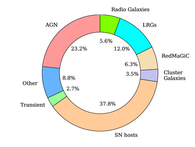
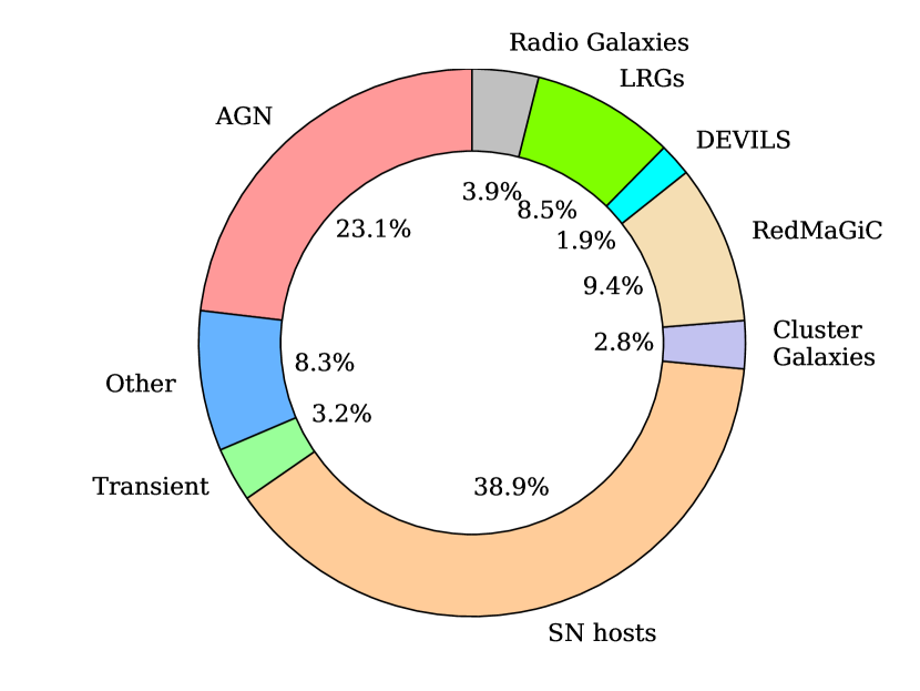
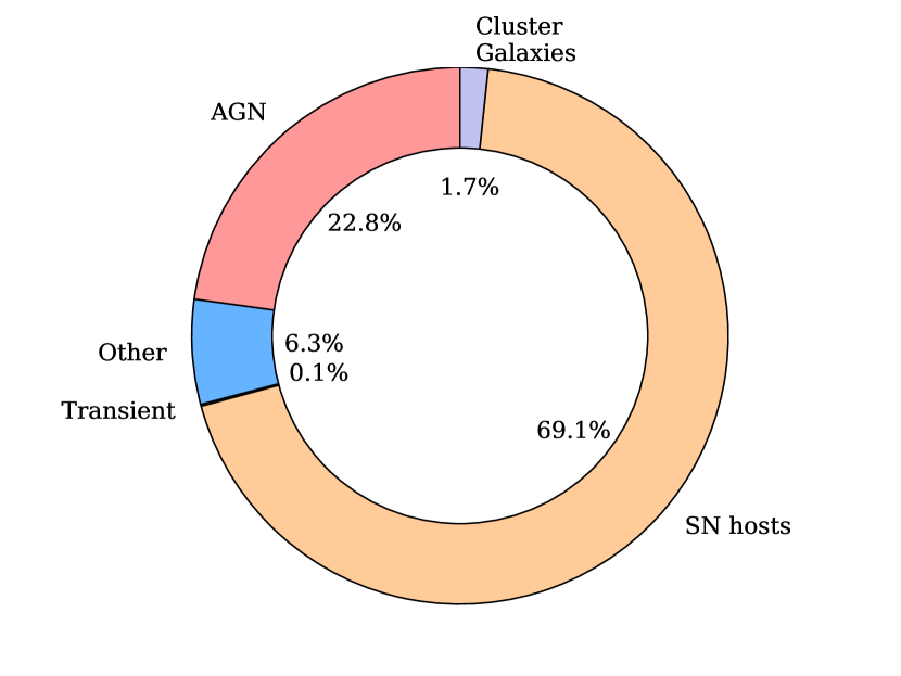
Fibre allocations for the last three years of OzDES are listed in Table 2 and shown as plots in Fig 1. A similar table in for the first three years is provided in Ch17. After Y1, a quarter of all fibres were allocated to AGN that were being followed in the OzDES reverberation mapping. The number of fibres allocated to SN hosts steadily increased from 12% in Y1 to 39% in Y5. The large jump from Y5 to Y6 in the number of SN hosts reflects the increased quota for SN hosts in Y6 and the addition of two new SN host categories. Almost all fibres in Y6 were allocated to an AGN or a SN host.
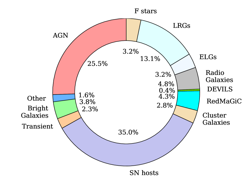
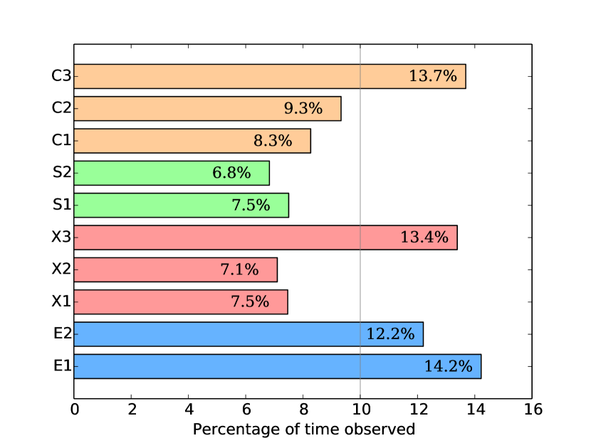
Fibre allocations over the full OzDES survey are shown in Fig 2. The three most commonly observed sources were SN hosts (35%), AGN (26%) and galaxies used to train photometric redshift algorithms: LRGs, ELGs, and redMaGiC galaxies (21%).
There can be considerable overlap in the individual target catalogues that make up the OzDES target input catalogue. For example, a SN host can also be listed as a radio galaxy, LRG, or redMaGiC galaxy. In Table 2, Fig 1, and Fig 2 objects retain the type that has the highest priority. For example, a source that is listed in the OzDES target input catalogue as a SN host, radio galaxy, an LRG, and a redMaGiC galaxy will be classified and counted as a SN host.
| Y4 | Y5 | Y6 | ||||
| Object | Fibre | Fraction of | Fibre | Fraction of | Fibre | Fraction of |
| Hours | Fibre Hours | Hours | Fibre Hours | Hours | Fibre Hours | |
| Transients | 939 | 2.7% | 1195 | 3.2% | 29 | 0.1% |
| AGN | 8191 | 23.2% | 8578 | 23.1% | 6115 | 22.8% |
| SN hosts | 13333 | 37.8% | 14413 | 38.9% | 18513 | 69.1% |
| Cluster Galaxies | 1219 | 3.5% | 1048 | 2.8% | 449 | 1.7% |
| Radio Galaxies | 1989 | 5.6% | 1455 | 3.9% | 0 | 0.0% |
| DEVILS | 0 | 0.0% | 720 | 1.9% | 0 | 0.0% |
| RedMaGiC | 2220 | 6.3% | 3481 | 9.4% | 0 | 0.0% |
| LRGs | 4235 | 12.0% | 3137 | 8.5% | 0 | 0.0% |
| Other | 3107 | 8.8% | 3071 | 8.3% | 1688 | 6.3% |
| Total | 35232 | 37097 | 26793 | |||
| All years | ||
| Object | Fibre | Fraction of |
| Hours | Fibre Hours | |
| Transients | 4438 | 2.3% |
| AGN | 49548 | 25.5% |
| SN hosts | 68028 | 35.0% |
| Cluster Galaxies | 5523 | 2.8% |
| DEVILS | 720 | 0.4% |
| Radio Galaxies | 9271 | 4.8% |
| RedMaGiC | 8394 | 4.3% |
| F stars | 6247 | 3.2% |
| LRGs | 25521 | 13.1% |
| ELGs | 6175 | 3.2% |
| Other | 3043 | 1.6% |
| Bright Galaxies | 7298 | 3.8% |
| Total | 194207 | |
3.3 Observing Strategy, Calibration and Data Reduction
During each run, we aimed to get at least two 2400 second exposures per field. This was not always possible due to the length of some runs and weather conditions. Of the 31 runs that were scheduled for OzDES, we were able to observe all 10 fields on 16 occasions. There were only two, relatively short runs where we did not observe any fields because of poor weather.
Overall, % of time was lost to poor observing conditions. Another % of the time was sub-optimal (thick cirrus and/or poor seeing), and was used for the back up programme. Observing logs for the final three years of OzDES, including the amount of time lost for poor weather, are included in the appendixes.
The two extra deep fields, C3 and X3, had the highest priority, so these fields were the most frequently observed, as can be seen in Fig. 3. The two E fields, E1 and E2 were also observed frequently, since these fields were often the only ones visible at the beginning of the night during the start of the observing season and are the most southern of the ten deep fields, which results in a longer window of observability from the AAT. Next in priority were the six remaining fields: X1, X2, C1, C2, S1, and S2.
In addition to the sources listed in Table 1, about a dozen fibres per field were allocated to F stars, and another 25 “sky” fibres were placed on positions that were free of sources. The targeting priority for both the F stars and the “sky” fibres was set to 5, which is below that of Transients, AGN and SN hosts, but higher than other types of objects. See Table 1 for details.
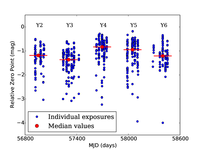
The F stars were primarily used to estimate throughput. The throughput was measured by integrating the extracted and wavelength calibrated spectra though the DECam filter band passes (Flaugher et al., 2015). For the red arm, we used the DECam filter: for the blue arm, we used the DECam filter. The relative throughput of the red arm over the course of OzDES is shown in Fig. 4. The throughput is reported in magnitudes, so each tick on the vertical access corresponds to a difference of about 2.5 in throughput. The vertical scatter is largely driven by transparency and atmospheric seeing.
Spectra that were taken when the throughput was excessively low (a couple of magnitudes lower than the medians shown in Fig. 4) are not used in the coadded spectra; however, they are included in the data release. For such spectra, the QC keyword in the FITS header is given the value poorConditions.
In the early years, we used the F-stars to derive the transfer functions for the red and blue arms that were then used throughout the survey, and to develop techniques that used the broadband DES photometry to spectrophotometrically calibrate the spectra of AGN used for the OzDES RM project (Hoormann et al., 2019).
All data were processed with the OzDES pipeline, which uses a modified copy of v6.46 of 2dfdr333https://aat.anu.edu.au/science/software/2dfdr (Croom et al., 2004) and our own bespoke python scripts. The steps are described in Yu15 and Ch17, so we do not repeat them here. Since Ch17, a small number of improvements to the pipeline have been made, the most significant of which were a more robust algorithm to determine the factor that scales spectra in the blue and red arms, modifications to the PCA sky subtraction algorithm to make it less sensitive to cosmic rays that were not fully masked, and more complete masking of artifacts. These artifacts are described in section C.3.
All data were processed at the telescope, and combined with data taken during earlier observing runs. Once processed, all raw and reduced files were then archived on a server in Canberra. Typically, this was done daily, after the night had ended, but before the start of the next night. After each field was processed, the data was made available for OzDES team members444Colloquially referred to as “redshifters.” dedicated to the task of measuring redshifts within 24 to 48 hours of the data being taken. With the exception of transients and AGN, sources with secure redshifts (see the next section) were removed from the target catalogues and not re-observed during subsequent nights. During some of the longer OzDES runs, we observed a number of the DES fields on multiple occasions. If this occurred, then all objects that were observed on the first occasion would be given higher priority in subsequent observations, unless they had a secure redshift and had been removed from the target catalogue. We have reprocessed all the data with the same version of the pipeline on a couple of occasions. This ensures that all data are processed in a consistent manner. The latest version of the OzDES pipeline is version 18.21, and all data presented in this paper have been processed with that version.
4 Redshifts
As noted in Ch17, redshifts have been measured using MARZ (Hinton et al., 2016) since the start of Y3. Earlier than this RUNZ, which was developed by Will Sutherland, had been used. Measuring redshifts is a task that is performed by two redshifters, whose results are collated, scrutinised and then merged by the chief redshift whip. Merging is also done using MARZ. The merged results then enter the OzDES database, from which all other products are derived.
OzDES uses a redshift flag to quantify the confidence that the reported redshift is correct. As reported in Yu15 and Ch17, the flag can take on five main values.
-
•
, redshift based on multiple strong spectroscopic features matched, % confidence.
-
•
, redshift based typically on a single strong spectroscopic feature or multiple weak features, % confidence.
-
•
, potential redshift associated with typically a single weak feature, low confidence, not to be used for science.
-
•
, no matching features, thus no constraints on redshift.
-
•
, securely classified star.
As the survey progressed, we monitored the growing redshift catalogue for sources that had conflicting redshifts. These are sources in which the redshift changes between observing runs but the redshift quality flag, , remains unchanged and . An example is a source that is assigned a redshift during one run, but with the addition of more data in a later run, is assigned a different redshift () with the same quality flag.
On two occasions, once at the end of Y4 once at the end of Y6 , we collated all cases where there was conflict, defined on these occasions having a redshift difference larger than 0.05, and reprocessed and re-redshifted these sources in the same way we redshifted sources during each observing run. The revised redshifts were then added to our redshift catalog. At the end of Y4, there were a total of 191 sources that had conflicting redshifts. At the end Y6, there were a total of 49, perhaps illustrating a degree of improvement by the human redshifters.
In preparation for the second OzDES data release, we revisited cases with conflicting redshifts, this time decreasing the threshold from 0.05 to 0.01 in redshift. We also included sources that were classified with quality redshift at some stage during the survey but ended up with a lower redshift quality flag once all data were combined. Combined, about 820 sources were re-examined.
4.1 Redshift Reliability
Using data taken up until the end of Y1, Yu15 estimated the reliability of redshifts that are assigned and using external catalogues and repeat observations of the same target. They find that quality redshifts are 100% reliable and quality redshifts are reliable. After Y1, a number of measures were put in place to lift the reliability of the quality redshifts. Our target for quality redshifts at the start of the OzDES survey was . As discussed below, we have reached this goal.
Ch17 used a different approach to assessing redshift reliability, taking advantage of the observing strategy applied to SN hosts. Unlike other target types, SN hosts were not removed from the input target catalogues until they attained a quality redshift. For those SN hosts with quality redshifts that initially attained a quality redshift, one can compare the initial redshift with the final redshift and get an estimate of reliability of the quality redshifts, assuming that the quality redshifts have a known reliability, which we take to be 100%, following that found in Yu15.
Using data up until the end of Y3, Ch17 found that the redshifts of 17 out 443 sources (3.8%) changed between the initial quality redshift and the final quality redshift. We repeated this analysis, using a sample that is almost five times larger. We find that 64 of 2093 sources (3.1%) changed redshifts, a slightly smaller fraction than found in Ch17. The results are shown in Fig. 5.

The SN hosts allow one to examine the reliability of the quality redshifts in a second, complimentary way. A number of the fainter SN hosts have been observed over several years and 20 or more observing runs. As more data were obtained and added to earlier data, they would have been re-redshifted, sometimes twice or more per run, which can occur if they were observed over multiple times during a run. Some sources have dozens of redshift measurements. Every time a source was redshifted, there is a chance of an erroneous redshift being assigned to that source. We can get a rough estimate of how often this happens by searching for objects that obtained a quality redshift during one run, but did not subsequently obtain a or quality redshift with more data.
We search the database for examples where a quality redshift was assigned once and not assigned again, even if the exposure time had increased by a factor of two or three by the end of Y6. For these two cases, we identified 31 and 11 SN hosts, respectively. For these sources, we reduce the redshift quality flag from to . However, this can only be applied to SN hosts, as all other objects are deselected from the input target catalogue once a quality redshift is obtained. There are 1100 SN hosts with a quality redshift, potentially indicating an error rate in addition to that noted above of 1-3%.
The SN hosts also allow one to get a handle on the repeatability of the redshift measurement. We first selected SN hosts that have at least four redshift measurements with a quality flag of 3 or 4. We then compute the RMS of the redshifts for each host. The median RMS is 0.00015. While this is indicative of the redshift uncertainty, it is likely that it is a lower limit, as the measurements are not fully independent: redshifts derived from data taken later include earlier data. Indeed, the median RMS is a factor of two smaller than the uncertainty reported in Yu15, who report 0.0003 for SN hosts using redshifts that were obtained from data that were fully independent.
The impact of a redshift uncertainty of 0.0003 on the dark energy equation of state parameter is negligible if the uncertainty is not systematic. If the uncertainty is systematic, then the dark energy equation of state parameter could be biased (Calcino & Davis, 2017).
4.2 Redshift Outcomes
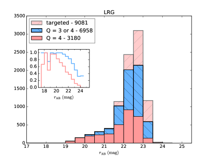
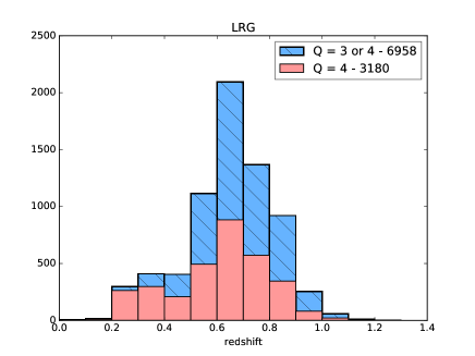
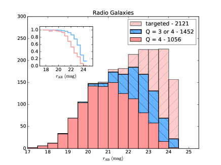
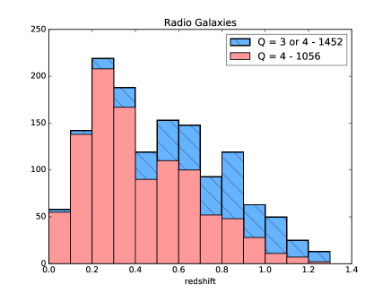
The diversity of objects that were observed over the six years by OzDES is large; from radio sources covering a broad range in magnitude and redshift, to more restricted classes of objects, such as LRGs, covering smaller magnitude and redshift ranges.
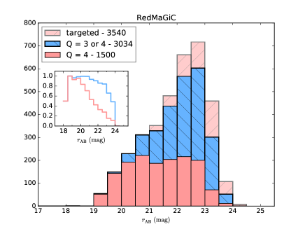
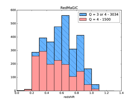
In Figs 6, 7, and 8, we provide magnitude and redshift distributions for RedMaGiC galaxies, LRGs and radio galaxies. As noted at the end of Sec. 3.2, some targets had multiple types. An LRG may have been classified as a redMaGiC galaxy and visa-versa. About 40% of all sources observed by OzDES had multiple types. In these plots, we include all objects of the indicated type, even if it also had another type.
Also shown as an insert to these figures and Fig. 10 is the redshift completeness, defined as the number of objects with a redshift divided by the number of objects that were targeted. A number of targets were spectroscopically classified as stars. These were removed before computing the redshift completeness.
4.3 Redshift Completeness
4.3.1 Completeness as a function of magnitude and exposure time
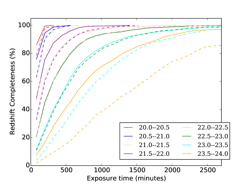
A little more than one third of the 192,000 fibre hours that were spent observing all targets were spent on SN hosts (see Table 3). SN hosts were targeted during the entire duration of OzDES and were not deselected from the input target catalogue until a quality redshift was obtained. They are therefore useful in examining how redshift completeness depends on magnitude and exposure time. However, caution is needed before applying the results from SN hosts to the general population of field galaxies, because SN hosts are a biased subset. SN hosts are more likely to be , and therefore within the spectral range covered by OzDES.
All SN hosts were selected on the basis of the detection of a transient in the DECam images. With the exception of super-luminous supernovae, which are rare, there would be few SN hosts that are at redshifts that places the [OII] Å doublet beyond the red end of the spectral range covered by the setting we used in AAOmega, which is at 8800Å. The red end corresponds to a redshift of for [OII]. Nearly all of the SN Ia detected by DES will be below this redshift (Bernstein et al., 2012). Hence, when interpreting the completeness of OzDES as a function of magnitude, the completeness will be different than for a survey that targeted field galaxies.
The redshift completeness of SN hosts as a function of exposure time is shown in Fig. 9. The completeness is shown for different magnitude bins and two redshift quality flags. As expected, completeness increases with exposure time and is highest for the brightest sources. It is also higher for lower quality redshift flags.
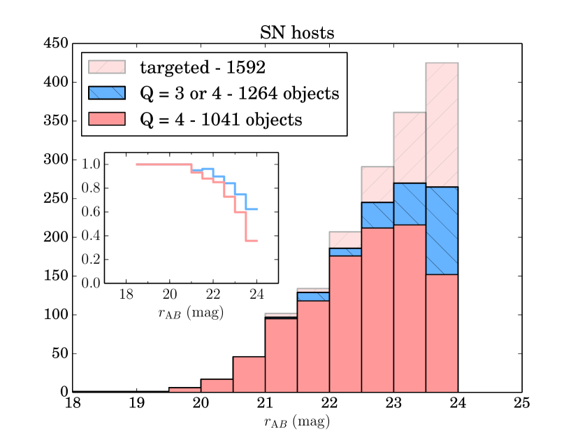
For the faintest bin (), the redshift completeness reaches % for quality 3 redshifts after 40 hours of integration. This does not mean that we reached this level of completeness in the survey, as not all SN hosts have been observed for that long. We anticipate that if we were to observe this long for all sources, then we would reach this level of completeness. As shown in Fig 10 the completeness in the faintest bin is 65%.
4.3.2 Completeness as a function of plate position
The positioning of fibres relies on a series of transformations between sky coordinates and plate coordinates. The transformations include the poscheck, which is updated by observatory staff, typically during the first night after 2dF is remounted on the telescope, and the plate survey, which is run every time a field is configured. The accuracy of these transformations has a direct impact on the amount of flux entering fibres and on the redshift completeness.
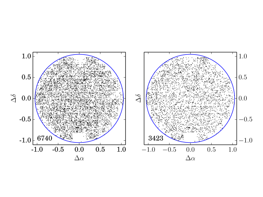
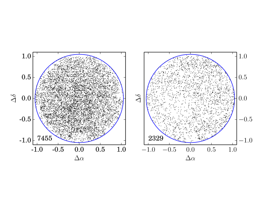
We examine how the redshift completeness varies across the field for SN hosts and LRGs. For LRGs, we include redMaGiC galaxies. Any variation in the redshift completeness across the field would be indicative of a problem in the accuracy of the transformations.
In the two panels of Fig. 11, we plot the position of SN hosts with and without redshifts, respectively. One can clearly see the boundary of the DECam chips traced by the SN hosts. The 10 fields in the DES deep survey were observed with minimal dithering. Consequently, chips gaps between the DECam CCDs were not covered and so no SNe are found in these gaps. A deficit of SN hosts can be seen in areas where CCDs were not functioning for some fraction of the survey.
Similarly, in the two panels of Fig. 12, we plot the position of LRGs with and without redshifts. The boundary of the DECam chips can no longer be seen, as LRGs were selected from imaging data that was more continuous.
The redshift completeness is shown for SN hosts and LRGs in Fig. 13. The completeness is not uniform for either class of object. In both cases, there is a drop towards the edge of the field. This is not unexpected and is due a drop in the image quality delivered by the 2dF corrector at the edge of the field and to the accuracy at which the plate can be rotated, which affects fibre near the field edge more than fibres in the centre. Less expected is a gradient from lower left to upper right in the redshift completeness of LRGs
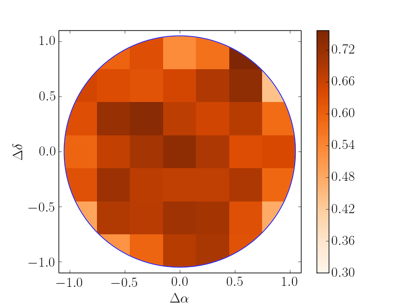
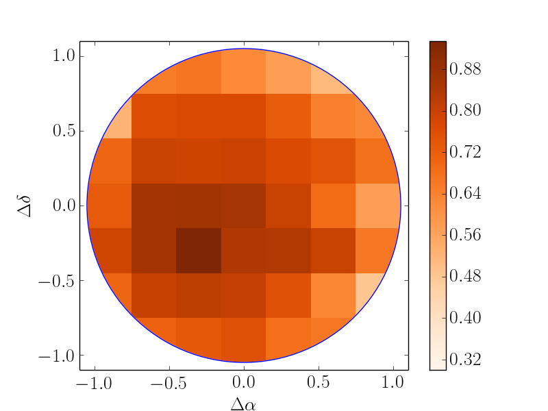
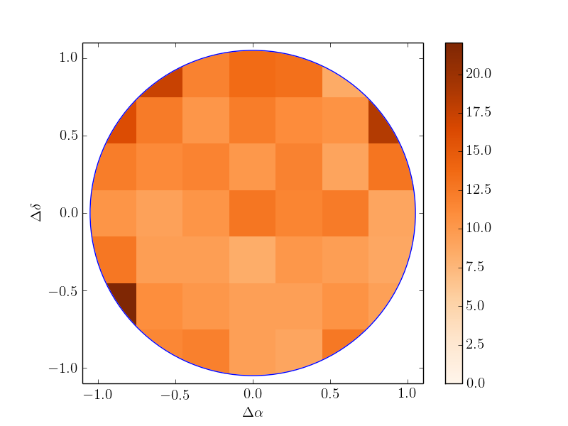
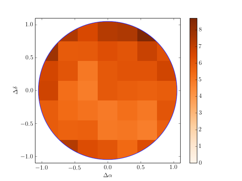
In Fig 14, we show the average number of exposures it takes to get a redshift. There is a general trend of increasing exposure time as one moves from the centre of the field-of-view to the edges. Again, the LRGs show a more significant gradient than the SN hosts.
There are a couple of potential reasons why the gradient is less significant for SN hosts. Firstly, SN hosts are not removed from the target catalogue until a secure, quality 4 redshift is obtained, whereas LRGs are removed from the target catalog once a quality 3 redshift is obtained. This will reduce field-dependent redshift incompleteness. Secondly, the flux lost due to fibre positioning errors is more severe for point sources than extended objects. LRGs due to their higher redshift and redder colours, will be more point like than SN hosts. At the AAT the profile of sources at these redshifts is dominated by the seeing, which will be better in the red than the blue.
The gradient has no impact on the primary OzDES science goals, as the spatial location of the AGN and SNe are not relevant, but the gradient needs to be taken into account if these data were to be used to estimate clustering from statistics such as the 2-point galaxy-galaxy correlation function.
5 The second OzDES Data Release
This paper marks the second OzDES release, which will be referred to as OzDES-DR2. OzDES-DR2 differs from OzDES-DR1555The redshift catalogue for OzDES-DR1 is available from https://datacentral.org.au., the first OzDES data release, in two key aspects.
-
•
The redshift catalogue includes all objects observed during the 6 years of OzDES and the OzDES pre-survey. This includes SN hosts, SNe, and targets for which a redshift could not be obtained.
-
•
The fully processed spectra are provided, including all individual spectra, as well as the stacked spectrum of each object.
In OzDES-DR2, we release 375,000 spectra of almost 39,000 objects, of which three quarters have a redshift with a quality flag of 3 or greater. We release all spectra, including the spectra of objects that do not have a redshift. These data can used to help secure redshifts for these objects if they are observed in the future with the AAT or other spectroscopic facilities. A full description of the data release is provided in Appendix C.
6 AGN reverberation mapping
Second to SN hosts, AGN were the next most frequently observed target type. As shown in Fig. 2, about a quarter of the fibre hours available to OzDES were allocated to the AGN reverberation mapping (RM) programme. The first year of the OzDES RM programme was used to define the sample that was followed in the subsequent five years. Details of the selection are provided in King et al. (2015). In brief, AGN were selected on the basis of the quality of the spectra that were taken in Y1, on the presence of emission lines, while avoiding AGN that occasionally fell in chip gaps, maximising the number of AGN with two reverberating spectral lines in our wavelength range, and ensuring that the AGN selected sampled the redshift interval . Most AGN that pass these cuts have have . From an initial sample of 3331 AGN, 771 AGN were followed during the next five years.
Apart from active transients, AGN in the OzDES RM sample have the highest priority, so the percentage of AGN that were allocated a fibre in any given observation was near to 100%. However, not all fields could be observed during every OzDES run, because of a combination of the finite duration of the observing runs, time lost to poor observing conditions, and the differing priority of the ten DES deep fields. Considering the latter and the bar chart shown in Fig. 3, we expect that the AGN in the two E-region fields and the X3 and C3 fields will have the greatest number of observations, both in terms of the raw number of times they were observed, and the number of runs in which they were observed.
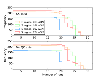
In Fig. 15, we show the distribution of the number of runs in which AGN were observed. Two plots are shown. In the lower plot, all observations are included, regardless of the observing conditions or the quality of the data. In the upper plot, only data that had a relative zero point greater than (see Fig. 4) and a quality control (QC) flag of ‘ok’ are included (see Appendix B for a discussion on the QC flag). The vertical solid line shows the number of runs on which OzDES observations were scheduled during the six years that OzDES ran. The two runs from the OzDES pre-survey are excluded, since the AGN RM pre-sample had not been defined at that time. This solid line represents an upper limit to the number of epochs. The median values for the four regions are shown in Table 4. The median values for the X and C regions include X3 and C3, which were the highest priority fields, so we list the median values for the C3 and X3 separately as well. For the E region fields and X3 and C3, the median is close to the 25 epochs that were used in the simulations of the OzDES RM programme in King et al. (2015).
With this number of epochs, simulations in King et al. (2015) predict that one should recover lags for 35-45% of the AGN depending on the accuracy with which one can calibrate the line flux. The simulations used a 10% accuracy for the line measurements. Hoormann et al. (2019) demonstrate that we are able to achieve this level of accuracy, so we anticipate that we will recover this fraction of lags in the two E fields and the C3 and X3 fields, and a lower fraction in the other six fields. The first two lags, using the CIV line and based on a subset of the OzDES data, were published in Hoormann et al. (2019).
| Fields | Epochs |
|---|---|
| C1, C2, and C3 | 23 |
| E1 and E2 | 24 |
| S1 and S2 | 18 |
| X1, X2, and X3 | 21 |
| C3 | 25 |
| X3 | 25 |
7 SN host galaxies: A case study
As illustrated in Fig. 2, slightly more than one-third of all the fibre hours allocated to targets during the six years of OzDES were allocated to SN hosts. Unlike other targets, SN hosts were observed until a secure redshift (see Sec. 4) was obtained. SN hosts also extend to fainter magnitudes than most targets. Both of these factors meant that the integration time for some hosts are very long, as long as 2 days in a number of cases.
We use SN hosts to examine how well the measured noise changes with time, and explore the implications of deselecting SN hosts once they reach a quality redshift and before they reach the more secure quality redshift.
7.1 Dependence on the measured noise with integration time
Ch17 showed that the noise in the spectra evolves with increasing exposure time, , according to expectations. The OzDES pipeline averages spectra from individual exposures rather than summing them, so the measured noise decrease as , or with the square root of the number of exposures if the exposure time is constant. Nearly all OzDES exposures were taken with an integration time of 40 minutes. We repeat the Ch17 analysis, which was done with just three years of OzDES data. With six years of data, there are more objects in total and there are more objects with longer integration times.
We do apply some qualitative cuts to the data chosen for this analysis. We exclude spectra that i) were taken in poor conditions (defined here as exposures that have a relative zero point of less than ; see Fig 4), ii) did not pass quality control, and iii) were taken during Y1 and SV. During Y1 and SV, we do not have reliable zero points, and did not take dome flats, so the quality of the processed data is not as good as it was in later years.
With these cuts, we then select SN hosts that have at least 12 exposures. This will tend to select SN hosts that are fainter than average, as redshifts for bright hosts would have typically been obtained with fewer exposures and would have been deselected from the target pool before 12 exposures had been taken. As the selected objects are faint, the signal to noise ratio is quite small, so spectral features do not contribute to the noise.
We then select a wavelength region over which to measure the noise. We start off with a region that is relatively free of night sky lines. The region we select starts at 6610Å and ends at 6750Å. We then examine how our results change if we choose a region that contains bright night sky lines.
We then randomise the order in which exposures were taken. The ordering is different for each object. For a given object, we take the first exposure and compute the clipped RMS over the wavelength region noted above. In computing the clipped RMS, we reject the 5 highest and 5 lowest values. Over the wavelength region that we sample, there are about 135 pixels, so the clipping removes less than 10% of the data. The clipping allows us to exclude residuals from cosmic rays that were not perfectly removed during the processing of the data and mitigates the effect of strong spectral features, such bright emission lines from the object. We experimented with the normalised median absolute deviation instead of the clipped RMS and obtained qualitatively similar results. All subsequent measurements of the clipped RMS are scaled by the clipped RMS that is computed in this first exposure.
We then add data from subsequent exposures in the randomised sequence, noting that we average the spectra, rather than summing them, and recompute the clipped RMS. This is done for every SN host. The results are shown in Fig 16.
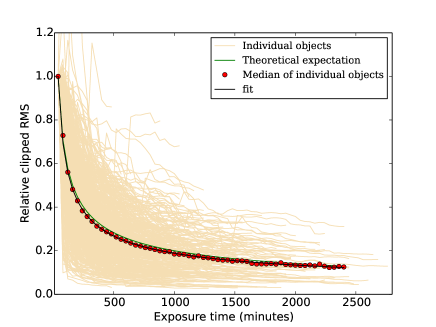
There is considerable scatter from object to object. This is caused by data of poorer than average quality entering the average at different stages of the sequence. For example, a sequence of exposures in which the first exposure is noisy will result in a much larger than anticipated drop in the relative clipped RMS when data of better quality is included. Applying stronger quality cuts reduces the scatter. To get an idea of the general trend, we take the median of all objects. These are the red circles in Fig. 16.
We fit the function
| (1) |
to the red points. The function equals 1 when , and allows for a noise floor. The theoretical expectation for Poisson noise is and . This is represented with the green curve. The best fit to Eq. 1 is the black curve. The best fit has and . The best fit is close to theoretical expectation for Poisson noise, and the floor is low. We find there is no reason to stop observing targets over the range of exposure times explored here. We will explore this point further in the next section.
There are limitations to our approach. Eq. 1 may not be the best functional form, and we have not allowed for the hard limits imposed by theory (i.e and ) when fitting Eq. 1. Indeed, we find . It is unclear what causes this.
We varied our selection cuts and repeated the analysis for the other fields to see how robust our results were. We do see some variability in the results, the origins of which are unclear. For the permutations we tried, we found and , i.e. a slightly steeper dependence than expected from theory and weak evidence for a noise floor. The floor is still less that the contribution from Poisson noise even after a day of exposure. At 1.5 days (which corresponds to 54 40-minute exposures), .
We also varied the wavelength region over which the statistics were computed, using both a region free of bright night sky lines (6610-6750 Å) and a region dominated by them (7700-8000 Å). In both cases, a dependence close to was observed.
7.2 Deselecting targets
It is clear that, for the range of exposure times explored in OzDES (up to two days of integration), the signal-to-noise continues to improve as expected, i.e. with the square root of the exposure time. If OzDES were to continue into the future, then exposure times could grow into many days. A number of questions then arise. How long should one spend on a target before deselecting it for a another one if one is unable to get a redshift, and is there a way of knowing if some targets are more likely to result in a redshift than others? Any decision to deselect one source in preference for another needs careful consideration, as such a decision will invariably lead to biases that need to be modelled.
During Y6, when 71% of the available fibre time was spent targeting SN hosts, there were more SN hosts without quality 4 redshifts than 2dF fibres, especially for C3 and X3, the two deepest DES fields. If there were many more fibres than the 392 available with 2dF, and SN hosts were the only targets, then the answer would be to continue observing these targets.
For instruments like 4MOST, which has 4 times as many fibres as 2dF, one could observe more targets longer without running out of fibres. Of course, 4MOST could choose to push to fainter limits than OzDES did (most OzDES hosts are brighter than ), in which case it too would have to make a choice about what to keep and what to drop in favour of something that has a higher chance of success.
Ultimately, this decision has to be based on the questions one is trying to address. A SN with a noisy light curve at may not be as valuable as two SNe with high quality light curves at a redshift of a half. We do not address this question in this paper, but leave it to when the DES 5-year photometrically selected sample is defined.
For SN hosts, there is an additional consideration. SN hosts are deselected once they get a quality redshift. Some SN hosts obtain a quality redshift relatively quickly, but fail to reach the quality redshift that is necessary for deselection. This raises an interesting question. How long should one continue observing such targets once the quality redshift is obtained?
We examine the number of exposures SN hosts remain at once that quality is obtained. We divide these objects into two. Those that eventually obtain a quality redshift and those that do not. Almost 85% of objects that move from to do so within 10 exposures of obtaining . If one were to deselect targets that fail to reach within 10 exposures of obtaining , then one would free up 6.6% of the fibre hours, which could then be used on other sources, at the cost of obtaining 6.2% fewer quality redshifts.
In OzDES, we did not deselect SN hosts before they reached , no matter how many exposures were being taken. We are now in position to explore how the choice of deselecting SN hosts biases the fitted cosmological parameters. This will be reported in a future paper.
About 35 SN hosts fainter the fail to obtain a quality redshift once a quality redshift was obtained, even after continuing to integrate for 30 or more exposures (equivalent to 20 hours of integration). We examined each of these sources, and found that more than half of them show a single bright line, which is assumed to be the [OII] doublet. These objects reach the level relatively quickly. The redshift of these sources is around one, meaning that other potential emission lines were outside the spectral range of AAOmega. During run041, we used a redder setting for AAOmega, which allowed us to pick up the [OIII] doublet in some cases. Most of the remaining cases consist of sources with weak features, typically a combination weak [OII], [OIII], and , that only start to become apparent after many hours of integration, but are not yet strong enough for a quality redshift to be assigned, even after an additional 20 hours of additional integration.
8 Implications for future surveys
By the early 2020s, LSST will have started surveying the Southern sky and several new multi-object spectroscopic facilities fed by rapidly configurable fibre positioners covering wide fields of view will be operational. Of the planned surveys using these new facilities, the Time-Domain Extragalactic Survey (TiDES, Swann et al., 2019), using 4MOST (de Jong et al., 2019) in combination with LSST, is the one that most closely matches the OzDES concept. A comparison of the OzDES and TiDES surveys is shown in Table 5. The survey characteristics of TiDES listed in Table 5 are subject to change as the survey strategy is still evolving.
| Metric | OzDES/AAT | TiDES/4MOST |
| Telescope, Spectrograph, and Positioner | ||
| M1 Diameter (m) | 3.9 | 4.2 |
| Field of view (sq. deg.) | 3.46 (circle) | 4.2 (hexagon) |
| Fibre diameter (″) | 2.0-2.1 | 1.45 |
| Number of fibres | 392 | 1624a |
| Config. time (min) | 40b | 2 |
| Spectral Resolution | 1400-1700 | 6500 |
| Wavelength range (Å) | 3700-8800 | 3700-9500 |
| Smallest sep. (″) | 30 | 15 |
| Survey characteristics | ||
| Survey regionc,d | DES deep fields | LSST DDF and |
| Median Seeing (″) | 1.5 | 0.8 |
| Usable clear fraction | 67% | 90% |
| Duration (years) | 5g | 5 |
| Transient redshifts | 5,000 | 50,000 |
| AGN monitored | 771 | 700 |
| Live transients | 1,450 | 30,000e |
| Fibre hours | 193,000 | 250,000 |
| Freq. (per lunation) | 1 | 2f |
| Observing season | 5 months | 9 monthsf |
| a Fibres feeding the two low-resolution spectrographs. | ||
| b Done in parallel while observing with the opposing plate. | ||
| c The 10 DES deep fields cover 27 sq. degrees. | ||
| d Deep Drilling Fields | ||
| e Mostly from the TiDES wide survey | ||
| f In the deep drilling fields. | ||
| g The SN programme in DES and OzDES lasted 5 seasons. | ||
On practically every metric, TiDES will be superior to OzDES. It will observe at least 10 times more live transients, mostly in the wide survey, it will measure up to 10 times more host galaxy redshifts, and it will monitor AGN at twice the frequency that OzDES did and with shorter seasonal gaps. TiDES will also observe transients over the majority of the southern sky, something that OzDES did not do.
Although the science goals and strategy of TiDES are heavily based upon that of OzDES, practically there are some differences. The first difference between OzDES and TiDES is that TiDES will not drive the pointings of 4MOST. Wherever 4MOST is scheduled to point there will be previously discovered transient targets, a majority of these targets anticipated to be discovered by LSST. If these transients are still bright enough to obtain a spectrum for spectral typing, TiDES will attempt do so. Otherwise TiDES will target the host galaxy of the transient to obtain a spectroscopic redshift for type Ia SN cosmology.
The second difference between OzDES and TiDES is that TiDES will have two components, a wide field component and a deep field component. The wide field follow-up will cover the majority of the southern sky, where low redshift transients and host galaxies will be targeted with a maximum exposure time of two hours. The second component to TiDES will be spectroscopic follow-up in the deep fields of 4MOST, where higher redshift live transients will be observed, the AGN reverberation mapping will take place, and where one can repeatedly target SN host galaxies to build up redshifts on the faintest of targets.
The 4MOST Deep fields currently correspond to four pointings, each covering 4.2 sq. degrees and contained within the LSST deep drilling fields (Guiglion et al., 2019). LSST data will provide the high precision photometry and high cadence light curves required for sub-percent precision cosmology. As three of the DES deep fields (ECDFS, XMM-LSS, ELAIS S1) are also covered by the 4MOST and LSST DDFs, this offers the exciting possibility of continued monitoring a subsample of the AGN observed by OzDES over a 15 year baseline, if the time gap between OzDES and TiDES can be covered. The higher cadence and longer observing season will also mean that TiDES will be more sensitive to AGN with shorter lags and less sensitive to seasonal gaps. Therefore TiDES will obtain a higher fraction of lags compared to OzDES.
With more than 4 times the number of fibres, and a field of view that is only slightly larger that 2dF, TiDES on 4MOST will be able to observe SN hosts in the deep fields longer without running out of fibres. Given the higher throughput, broader spectral coverage, and higher spectral resolution of 4MOST compared to AAOmega, and the better observing conditions on Cerro Paranal compared to Siding Spring, TiDES will be able to obtain host galaxy redshifts more quickly and to a fainter magnitude limit than OzDES.
9 Summary
Over six consecutive observing seasons, starting in 2013, OzDES obtained over 375,000 spectra of almost 39,000 sources in the ten DES deep fields. These spectra were obtained with the 2dF fibre positioner and AAOmega spectrograph on the AAT. Over that time, each DES SN field was observed between 18 and 25 times.
In these fields, OzDES has obtained redshifts for almost 7,000 galaxies that hosted a transient, and classified almost 270 transients. The strategy of targeting each field repeatedly has enabled redshifts to be obtained for sources as faint as . We show that one is not limited by a noise floor, even after two days of exposure, and that one can reach high spectroscopic completeness at these faint limits.
The strategy of targeting each field repeatedly has allowed OzDES to monitor 771 AGN. These data will be used to measure the lag between the continuum from the accretion disk and the broad lines from the broad line emission region. We anticipate that we will recover lags and derive black hole masses for approximately 30% of the AGN we monitored.
The OzDES observing strategy allowed a number of science programmes to run in parallel. Just over 60% of the 192,000 fibre hours were allocated to monitoring AGN and obtaining redshifts for galaxies that hosted a transient. The remaining 40% was used to obtain redshifts for wide variety of targets, such as radio galaxies, cluster galaxies, and galaxies to train photometric redshift algorithms.
OzDES can be used as a template for future surveys that use the next generation of wide-field multi-object fibre-fed spectroscopic facilities to target and monitor sources in the LSST deep drilling fields. These new facilities will have up to an order of magnitude more fibres than 2dF, and they will enable one to follow a larger number of fainter sources more frequently and for longer.
Acknowledgments
Parts of this research were supported by the Australian Research Council under grants DP160100930, FL180100168, and FT140101270.
Based in part on data acquired at the Anglo-Australian Telescope, under programme A/2013B/012. We acknowledge the traditional owners of the land on which the AAT stands, the Gamilaraay people, and pay our respects to elders past, present, and emerging.
We acknowledge the support of James Tocknell and Simon O’Toole from Data Central in helping us prepare OzDES-DR2.
L.G. was funded by the European Union’s Horizon 2020 research and innovation programme under the Marie Skłodowska-Curie grant agreement No. 839090.
F.H.P. was supported by an Australian Government Research Training Programme Scholarship.
Funding for the DES Projects has been provided by the U.S. Department of Energy, the U.S. National Science Foundation, the Ministry of Science and Education of Spain, the Science and Technology Facilities Council of the United Kingdom, the Higher Education Funding Council for England, the National Center for Supercomputing Applications at the University of Illinois at Urbana-Champaign, the Kavli Institute of Cosmological Physics at the University of Chicago, the Center for Cosmology and Astro-Particle Physics at the Ohio State University, the Mitchell Institute for Fundamental Physics and Astronomy at Texas A&M University, Financiadora de Estudos e Projetos, Fundação Carlos Chagas Filho de Amparo à Pesquisa do Estado do Rio de Janeiro, Conselho Nacional de Desenvolvimento Científico e Tecnológico and the Ministério da Ciência, Tecnologia e Inovação, the Deutsche Forschungsgemeinschaft and the Collaborating Institutions in the Dark Energy Survey.
The Collaborating Institutions are Argonne National Laboratory, the University of California at Santa Cruz, the University of Cambridge, Centro de Investigaciones Energéticas, Medioambientales y Tecnológicas-Madrid, the University of Chicago, University College London, the DES-Brazil Consortium, the University of Edinburgh, the Eidgenössische Technische Hochschule (ETH) Zürich, Fermi National Accelerator Laboratory, the University of Illinois at Urbana-Champaign, the Institut de Ciències de l’Espai (IEEC/CSIC), the Institut de Física d’Altes Energies, Lawrence Berkeley National Laboratory, the Ludwig-Maximilians Universität München and the associated Excellence Cluster Universe, the University of Michigan, the National Optical Astronomy Observatory, the University of Nottingham, The Ohio State University, the University of Pennsylvania, the University of Portsmouth, SLAC National Accelerator Laboratory, Stanford University, the University of Sussex, Texas A&M University, and the OzDES Membership Consortium.
Based in part on observations at Cerro Tololo Inter-American Observatory, National Optical Astronomy Observatory, which is operated by the Association of Universities for Research in Astronomy (AURA) under a cooperative agreement with the National Science Foundation.
The DES data management system is supported by the National Science Foundation under Grant Numbers AST-1138766 and AST-1536171. The DES participants from Spanish institutions are partially supported by MINECO under grants AYA2015-71825, ESP2015-66861, FPA2015-68048, SEV-2016-0588, SEV-2016-0597, and MDM-2015-0509, some of which include ERDF funds from the European Union. IFAE is partially funded by the CERCA programme of the Generalitat de Catalunya. Research leading to these results has received funding from the European Research Council under the European Union’s Seventh Framework Program (FP7/2007-2013) including ERC grant agreements 240672, 291329, and 306478. We acknowledge support from the Brazilian Instituto Nacional de Ciência e Tecnologia (INCT) e-Universe (CNPq grant 465376/2014-2).
This manuscript has been authored by Fermi Research Alliance, LLC under Contract No. DE-AC02-07CH11359 with the U.S. Department of Energy, Office of Science, Office of High Energy Physics. The United States Government retains and the publisher, by accepting the article for publication, acknowledges that the United States Government retains a non-exclusive, paid-up, irrevocable, world-wide license to publish or reproduce the published form of this manuscript, or allow others to do so, for United States Government purposes.
We are grateful for the extraordinary contributions of our CTIO colleagues and the DECam Construction, Commissioning and Science Verification teams in achieving the excellent instrument and telescope conditions that have made this work possible. The success of this project also relies critically on the expertise and dedication of the DES Data Management group.
References
- Angus et al. (2019) Angus C. R., et al., 2019, MNRAS, 487, 2215
- Astier et al. (2006) Astier P., et al., 2006, A&A, 447, 31
- Bernstein et al. (2012) Bernstein J. P., et al., 2012, ApJ, 753, 152
- Betoule et al. (2014) Betoule M., et al., 2014, A&A, 568, A22
- Bonnett et al. (2016) Bonnett C., et al., 2016, Phys. Rev. D, 94, 042005
- Calcino & Davis (2017) Calcino J., Davis T., 2017, J. Cosmology Astropart. Phys., 2017, 038
- Calcino et al. (2018) Calcino J., et al., 2018, The Astronomer’s Telegram, 11146, 1
- Childress et al. (2017) Childress M. J., et al., 2017, MNRAS, 472, 273
- Croom et al. (2004) Croom S., Saunders W., Heald R., 2004, Anglo-Australian Observatory Epping Newsletter, 106, 12
- D’Andrea et al. (2018) D’Andrea C. B., et al., 2018, arXiv e-prints,
- DESI Collaboration (2016) DESI Collaboration 2016, arXiv e-prints,
- Dark Energy Survey (2016) Dark Energy Survey 2016, MNRAS, 460, 1270
- Dark Energy Survey (2019a) Dark Energy Survey 2019a, Phys. Rev. Lett., 122, 171301
- Dark Energy Survey (2019b) Dark Energy Survey 2019b, ApJ, 872, L30
- Davies et al. (2018) Davies L. J. M., et al., 2018, MNRAS, 480, 768
- Dawson et al. (2009) Dawson K. S., et al., 2009, AJ, 138, 1271
- Diehl et al. (2018) Diehl H. T., et al., 2018, in Proc. SPIE. p. 107040D, doi:10.1117/12.2312113
- Flaugher et al. (2015) Flaugher B., et al., 2015, AJ, 150, 150
- Franzen et al. (2015) Franzen T. M. O., et al., 2015, MNRAS, 453, 4020
- Gschwend et al. (2018) Gschwend J., et al., 2018, Astronomy and Computing, 25, 58
- Guiglion et al. (2019) Guiglion G., et al., 2019, The Messenger, 175, 17
- Hinton et al. (2016) Hinton S. R., Davis T. M., Lidman C., Glazebrook K., Lewis G. F., 2016, Astronomy and Computing, 15, 61
- Hoormann et al. (2019) Hoormann J. K., et al., 2019, MNRAS, 487, 3650
- Jacobs et al. (2019) Jacobs C., et al., 2019, MNRAS, 484, 5330
- Johnson et al. (2017) Johnson A., et al., 2017, MNRAS, 465, 4118
- Khain et al. (2018) Khain T., et al., 2018, AJ, 156, 273
- King et al. (2015) King A. L., et al., 2015, MNRAS, 453, 1701
- LSST Science Collaboration (2017) LSST Science Collaboration 2017, arXiv e-prints,
- Lawrence et al. (2018) Lawrence J., et al., 2018, in Proc. SPIE. p. 10702A6, doi:10.1117/12.2314178
- Li et al. (2019) Li T. S., et al., 2019, MNRAS, 490, 3508
- Marshall et al. (2019) Marshall J., et al., 2019, ApJ, 882, 177
- Mudd et al. (2018) Mudd D., et al., 2018, ApJ, 862, 123
- Nord et al. (2016) Nord B., et al., 2016, ApJ, 827, 51
- Palmese et al. (2017) Palmese A., et al., 2017, ApJ, 849, L34
- Pierre et al. (2016) Pierre M., et al., 2016, A&A, 592, A1
- Prat et al. (2018) Prat J., et al., 2018, Phys. Rev. D, 98, 042005
- Pursiainen et al. (2018) Pursiainen M., et al., 2018, MNRAS, 481, 894
- Rozo et al. (2016) Rozo E., et al., 2016, MNRAS, 461, 1431
- Sánchez et al. (2014) Sánchez C., et al., 2014, MNRAS, 445, 1482
- Smith et al. (2018) Smith M., et al., 2018, ApJ, 854, 37
- Swann et al. (2019) Swann E., et al., 2019, The Messenger, 175, 58
- Tamura et al. (2018) Tamura N., et al., 2018, in Ground-based and Airborne Instrumentation for Astronomy VII. p. 107021C, doi:10.1117/12.2311871
- The MSE Science Team et al. (2019) The MSE Science Team et al., 2019, arXiv e-prints,
- Vargas-Magana et al. (2019) Vargas-Magana M., Brooks D. D., Levi M. M., Tarle G. G., 2019, arXiv e-prints,
- Webb et al. (2015) Webb T. M. A., et al., 2015, ApJ, 814, 96
- Wilson et al. (2009) Wilson G., et al., 2009, ApJ, 698, 1943
- Yasuda et al. (2019) Yasuda N., et al., 2019, PASJ, 71, 74
- Yu et al. (2020) Yu Z., et al., 2020, ApJS, 246, 16
- Yuan et al. (2015) Yuan F., et al., 2015, MNRAS, 452, 3047
- de Jong et al. (2019) de Jong R. S., et al., 2019, The Messenger, 175, 3
Appendix A Author Affiliations
1 The Research School of Astronomy and Astrophysics, Australian National University, ACT 2601, Australia
2 School of Mathematics and Physics, University of Queensland, Brisbane, QLD 4072, Australia
3 The Observatories of the Carnegie Institution for Science, 813 Santa Barbara St., Pasadena, CA 91101, USA
4 Centro de Investigaciones Energéticas, Medioambientales y Tecnológicas (CIEMAT), Madrid, Spain
5 School of Natural Sciences, College of Sciences and Engineering, University of Tasmania, Private Bag 37, Hobart TAS 7001, Australia
6 NASA Einstein Fellow
7 Department of Physics and Astronomy, University of Pennsylvania, Philadelphia, PA 19104, USA
8 INAF, Astrophysical Observatory of Turin, I-10025 Pino Torinese, Italy
9 School of Physics and Astronomy, University of Southampton, Southampton, SO17 1BJ, UK
10 Santa Cruz Institute for Particle Physics, Santa Cruz, CA 95064, USA
11 PITT PACC, Department of Physics and Astronomy, University of Pittsburgh, Pittsburgh, PA 15260, USA
12 Centre for Astrophysics & Supercomputing, Swinburne University of Technology, Victoria 3122, Australia
13 Department of Astronomy and Astrophysics, University of Chicago, Chicago, IL 60637, USA
14 Kavli Institute for Cosmological Physics, University of Chicago, Chicago, IL 60637, USA
15 Lawrence Berkeley National Laboratory, 1 Cyclotron Road, Berkeley, CA 94720, USA
16 School of Physics, University of Melbourne, Parkville, VIC 3010, Australiaa
17 Department of Physics, University of Michigan, Ann Arbor, MI 48109, USA
18 Australian Astronomical Optics, Macquarie University, North Ryde, NSW 2113, Australia
19 Lowell Observatory, 1400 Mars Hill Rd, Flagstaff, AZ 86001, USA
20 Centre for Extragalactic Astronomy, Department of Physics, Durham University, Durham DH1 3LE, UK
21 Institute for Computational Cosmology, Durham University, South Road, Durham DH1 3LE, UK
22 Sydney Institute for Astronomy, School of Physics, A28, The University of Sydney, NSW 2006, Australia
23 Institute of Cosmology and Gravitation, University of Portsmouth, Portsmouth, PO1 3FX, UK
24 Center for Cosmology and Astro-Particle Physics, The Ohio State University, Columbus, OH 43210, USA
25 Department of Astronomy, The Ohio State University, Columbus, OH 43210, USA
26 Université Clermont Auvergne, CNRS/IN2P3, LPC, F-63000 Clermont-Ferrand, France
27 School of Science, UNSW Canberra, Australian Defence Force Academy, Canberra 2612, Australia
28 Korea Astronomy and Space Science Institute, 776 Daedeokdae-ro, Yuseong-gu, 34055 Daejeon, Republic of Korea
29 Centre for Translational Data Science, University of Sydney, Darlington NSW 2008
30 Department of Physics, Duke University Durham, NC 27708, USA
31 Cerro Tololo Inter-American Observatory, National Optical Astronomy Observatory, Casilla 603, La Serena, Chile
32 Departamento de Física Matemática, Instituto de Física, Universidade de São Paulo, CP 66318, São Paulo, SP, 05314-970, Brazil
33 Laboratório Interinstitucional de e-Astronomia - LIneA, Rua Gal. José Cristino 77, Rio de Janeiro, RJ - 20921-400, Brazil
34 Fermi National Accelerator Laboratory, P. O. Box 500, Batavia, IL 60510, USA
35 Instituto de Fisica Teorica UAM/CSIC, Universidad Autonoma de Madrid, 28049 Madrid, Spain
36 CNRS, UMR 7095, Institut d’Astrophysique de Paris, F-75014, Paris, France
37 Sorbonne Universités, UPMC Univ Paris 06, UMR 7095, Institut d’Astrophysique de Paris, F-75014, Paris, France
38 Department of Physics and Astronomy, Pevensey Building, University of Sussex, Brighton, BN1 9QH, UK
39 Department of Physics & Astronomy, University College London, Gower Street, London, WC1E 6BT, UK
40 Department of Astronomy, University of Illinois at Urbana-Champaign, 1002 W. Green Street, Urbana, IL 61801, USA
41 National Center for Supercomputing Applications, 1205 West Clark St., Urbana, IL 61801, USA
42 Institut de Física d’Altes Energies (IFAE), The Barcelona Institute of Science and Technology, Campus UAB, 08193 Bellaterra (Barcelona) Spain
43 Institut d’Estudis Espacials de Catalunya (IEEC), 08034 Barcelona, Spain
44 Institute of Space Sciences (ICE, CSIC), Campus UAB, Carrer de Can Magrans, s/n, 08193 Barcelona, Spain
45 INAF-Osservatorio Astronomico di Trieste, via G. B. Tiepolo 11, I-34143 Trieste, Italy
46 Institute for Fundamental Physics of the Universe, Via Beirut 2, 34014 Trieste, Italy
47 Observatório Nacional, Rua Gal. José Cristino 77, Rio de Janeiro, RJ - 20921-400, Brazil
48 Department of Astronomy/Steward Observatory, University of Arizona, 933 North Cherry Avenue, Tucson, AZ 85721-0065, USA
49 Jet Propulsion Laboratory, California Institute of Technology, 4800 Oak Grove Dr., Pasadena, CA 91109, USA
50 Department of Physics, Stanford University, 382 Via Pueblo Mall, Stanford, CA 94305, USA
51 Kavli Institute for Particle Astrophysics & Cosmology, P. O. Box 2450, Stanford University, Stanford, CA 94305, USA
52 SLAC National Accelerator Laboratory, Menlo Park, CA 94025, USA
53 Département de Physique Théorique and Center for Astroparticle Physics, Université de Genève, 24 quai Ernest Ansermet, CH-1211 Geneva, Switzerland
54 Department of Physics, ETH Zurich, Wolfgang-Pauli-Strasse 16, CH-8093 Zurich, Switzerland
55 Department of Physics, The Ohio State University, Columbus, OH 43210, USA
56 Center for Astrophysics Harvard & Smithsonian, 60 Garden Street, Cambridge, MA 02138, USA
57 Department of Astrophysical Sciences, Princeton University, Peyton Hall, Princeton, NJ 08544, USA
58 Observatories of the Carnegie Institution for Science, 813 Santa Barbara St., Pasadena, CA 91101, USA
59 George P. and Cynthia Woods Mitchell Institute for Fundamental Physics and Astronomy, and Department of Physics and Astronomy, Texas A&M University, College Station, TX 77843, USA
60 Institució Catalana de Recerca i Estudis Avançats, E-08010 Barcelona, Spain
61 Instituto de Física, UFRGS, Caixa Postal 15051, Porto Alegre, RS - 91501-970, Brazil
62 Computer Science and Mathematics Division, Oak Ridge National Laboratory, Oak Ridge, TN 37831
63 Max Planck Institute for Extraterrestrial Physics, Giessenbachstrasse, 85748 Garching, Germany
64 Universitäts-Sternwarte, Fakultät für Physik, Ludwig-Maximilians Universität München, Scheinerstr. 1, 81679 München, Germany
Appendix B Observing logs for Y4, Y5 and Y6
The observing logs for Y4, Y5, and Y6 are shown in Tables B, B, and B, respectively. They follow the format presented in Yu15 and Ch17. The MaxVis field (Yu et al., 2020) was observed for 155 minutes during run 28 on 25 and 26 December 2017.
| UT Date | Observing runa | Total exposure time (minutes) | Notes for entire run | |||||||||
| E1 | E2 | S1 | S2 | C1 | C2 | C3 (deep) | X1 | X2 | X3 (deep) | |||
| 2016-08-25 | 024 | 80 | - | - | - | - | - | - | - | - | - | 0.5/1.5 clear nights |
| 2016-08-26 | - | 90 | - | - | - | - | - | - | - | - | ||
| 2016-08-27 | - | - | - | - | - | - | - | - | - | 110 | ||
| 2016-08-28 | - | - | - | 85 | - | - | - | - | - | - | ||
| 2016-08-29 | 180 | - | - | - | - | - | 80 | 80 | - | - | ||
| 2016-09-25 | 025 | - | 80 | - | - | - | 20 | 120 | - | - | 120 | 3.5/4.5 clear nights |
| 2016-09-26 | 80 | - | - | - | 30 | 120 | - | 120 | - | - | ||
| 2016-09-27 | - | 80 | 40 | - | 80 | - | - | - | 120 | - | ||
| 2016-10-05 | - | 40 | 100 | 120 | - | - | - | - | - | - | ||
| 2016-10-31 | 026 | - | - | - | - | - | - | 80 | - | - | 120 | 3.3/3.5 clear nights |
| 2016-11-01 | 120 | - | 120 | - | - | - | 60 | - | - | 120 | ||
| 2016-11-02 | - | 120 | - | 120 | - | - | - | 80 | - | - | ||
| 2016-11-03 | 80 | - | - | - | 120 | 110 | - | - | 120 | - | ||
| 2016-11-25 | 027 | 120 | - | - | - | 40 | - | 120 | - | - | 120 | 5.0/5.0 clear nights |
| 2016-11-26 | - | 120 | 120 | - | - | 120 | - | - | - | - | ||
| 2016-11-27 | - | - | - | 120 | 120 | - | - | 120 | - | - | ||
| 2016-11-28 | - | - | 120 | - | - | 68 | 80 | - | 120 | - | ||
| 2016-11-29 | 120 | - | - | - | - | 153 | - | - | - | 120 | ||
| 2016-12-25 | 028 | - | - | - | - | - | 80 | 80 | - | - | 120 | 2.8/4.0 clear nights |
| 2016-12-26 | - | - | 80 | - | 80 | - | - | - | 80 | - | ||
| 2016-12-27 | - | - | - | 80 | - | - | 80 | 80 | - | - | ||
| All Y4 | Total(min) | 780 | 530 | 580 | 525 | 470 | 671 | 700 | 480 | 440 | 830 | |
a Run numbering includes runs from 2dFLenS and DEVILS projects, so is not necessarily contiguous. b Bright object backup programme for poor conditions, not counted toward final total.
b Bright object backup programme for poor conditions, not counted toward final total.
b Bright object backup programme for poor conditions, not counted toward final total.
Appendix C The second OzDES Data release - OzDES-DR2
The second OzDES data release, OzDES-DR2, consists of the OzDES redshift catalogue and the reduced spectra. The data are available from Data Central666https://datacentral.org.au.
C.1 Redshift Catalogue
The OzDES-DR2 redshift catalogue is a FITS binary table containing almost 38,700 entries, of which almost 30,000 have a redshift with quality flag 3 or greater. The columns in the catalogue are described in Table 9.
The transient type is sourced from the 34 ATels (e.g., Calcino et al., 2018) that OzDES published over 6 years. D’Andrea et al. (2018) provides a description off how transients are classified.
When available, we add comments made by redshifters. Not all sources have comments, as adding a comment was left to the discretion of the redshifter.
Many sources were assigned multiple types. For example, sources that were assigned the LRG type were often assigned as redMaGiC sources and visa-versa. Sources observed during the OzDES pre-survey (runs 001 and 002) were not given an object type.
| Name | Description | Units |
| OzDES ID | Official DES name or an assigned OzDES name | … |
| if an official DES name is unavailable | … | |
| Alpha J2000 | Right Ascension | deg |
| Delta J2000 | Declination | deg |
| rmag | band magnitude | … |
| Redshift; -9.99 means no redshift | … | |
| qop (Q) | Redshift quality flag | … |
| Object types | Assigned types | … |
| Transient type | Type of transient (e.g. SN Ia, SN II, etc.); Assigned to None if no type | … |
| Comment | Comments from redshifters | … |
C.2 Spectra
All spectra are provided as multi-extension FITS. For targets observed up to and including run 40, there is usually one FITS file per target. If a target was also observed during run 41, which used a redder setting for AAOmega, we provide a second FITS file containing the data from that run combined with data from earlier runs. A small number of targets in run 41 were only observed in that run. In this case, there is just one FITS file per target.
Within each FITS file, there are extensions containing the stacked spectrum and the spectra that went into the stack. Also included are the variances and bad pixel masks for each spectrum. The extensions are described in Table 10. The individual spectra that go into the stack are ordered by date, from the one taken first to the last.
All spectra have been shifted to the heliocentric reference frame.
| Extension | Description |
|---|---|
| Primary | Stacked spectrum |
| 1 | Variance spectrum |
| 2 | Mask |
| 3 | Spectrum of first epoch |
| 4 | Variance spectrum of first epoch |
| 5 | Mask for first epoch |
| Spectrum of ith epoch | |
| Variance spectrum of ith epoch | |
| Mask for ith epoch |
The keywords in the FITS headers are described in Table 11.
| Primary Headera | |
|---|---|
| DO_HELIO | An internal flag recognised by the redshift code MARZ that ensures that no helio-centric |
| correction is applied by MARZ when set to false | |
| NDATE | The date the data were combined |
| SOURCE | The original source name |
| VERCOADD | The version of the coadd pipeline that stacks the reduced data |
| RMAG | band magnitude in a 2″ aperture |
| TYPEn | Target type |
| Z | redshift; -9.99 means no redshift |
| QOP | redshift quality flag |
| Individual epochsb | |
| REDZPd | The zero point in the -band. Measured from the spectra of F stars that were observed |
| at the same time as the source | |
| REDSENSF | The sensitivity function used in the red arm |
| BLUEZP | The zero point in the -band. Measured from the spectra of F stars that were observed |
| at the same time as the source | |
| BLUSENSF | The sensitivity function used in the blue arm |
| QC | Quality control flag |
| VERSION | The version of the pipeline that processes the raw data and produces single epoch reduced spectra |
| INCOADD | True if the epoch is included in the coadd |
| PIVOT | The 2dF fibre number |
| XPLATE | The X position on the plate (microns) |
| YPLATE | The Y position on the plate (microns) |
| ORIGTARG | The name of the target used in this observation |
| SOURCEF | The raw data filename (red arm only) |
| FLXSCALE | The scale factor that was applied in the co-adding |
| FLSCTYPE | The method used to compute scale factor |
| RMAG | in the input target catalogue |
| Individual epochsc | |
| EXPOSED | Exposure time |
| DICHROIC | Dichroic used - x6700 for run041, x5700 otherwise |
| SOURCE | 2dF field plate - either plate 0 or plate 1 |
| UTMJD | Modified Julian Date |
| ZDSTART | Zenith Distance at the start of the exposure |
| ZDEND | Zenith Distance at the end of the exposure |
| a Keywords that are in the FITS standard are not listed. | |
| b Keywords that are inserted when the data are co-added. | |
| c Keywords that are part of the header produced at the telescope and keywords. Not all keywords are listed. | |
| d Zero points are defined as , where is the catalog magnitude of the F star and is the observed | |
| spectrum integrated over the band for the blue arm and the band for the red arm. | |
C.3 Data Quality
The quality of the data is characterised in a couple of ways. The keywords REDZP and BLUEZP give an indication of the observing conditions at the time the data were taken. They are determined from F stars that were observed at the same time as the target. For the red arm, a zero point that is smaller than 31 usually means that conditions were poor, which could be due to seeing or the presence of cloud. It could also be due to an exposure that was cut short.
Most of the 375,000 spectra in the data release have been visually inspected and problematic cases noted in the QC keyword. As this is not 100% foolproof, there might be a number of problematic cases that have been missed. A value for QC that differs from “ok” indicates that there is a problem with the spectrum. The nature of the problem is noted in the value of the QC keyword and is described in Table 12.
Some of the problems are caused by artifacts that affect a limited wavelength range. Others affect the whole spectrum. The region of the spectrum affected by the artifact is noted in the masks. A value of 1 in the mask marks the region of poor quality data.
Examples of what the artifacts look like are available from the OzDES-DR2 documentation page at Data Central.
| QC value | Description |
|---|---|
| 700nmLED | Contamination from an LED in the gripper arm. This was discovered a few years, |
| into the survey, so it mostly affects early data. | |
| redDip | Most likely associated to charge traps in the old AAOmega red CCD. Affects data taken prior |
| to run007. | |
| doubleDip_1 | Most likely associated to charge traps in the old AAOmega red CCD. Affects data taken prior |
| to run007. | |
| doubleDip_2 | Most likely associated to charge traps in the old AAOmega red CCD. Affects data taken prior |
| to run007. | |
| doubleHump | Origin unknown. |
| fib388p0 | Issues with fibre 388 on plate 0. Cause unknown. |
| fib94p1 | Issues with fibre 94 on plate 1. Cause unknown. |
| redfail | Failed reduction in red arm. |
| redPCAFail | Failed PCA sky subtraction in the red arm. |
| bluefail | Failed reduction in blue arm. |
| failedReduction | Failed reduction, both arms. |
| redPCAfail | Failed PCA sky subtraction in red arm. |
| brightStarBlue | A bright star in a nearby fibre causes the reduction in the blue arm to fail or contaminates the |
| extracted spectrum in the blue arm. | |
| brightStarRed | As above, but for the red arm. |
| brightStarAll | As above, but for the entire spectrum. |
| fringed | Fringes detected. |
| poorConditions | Poor observing conditions. |
| blueSkySubFail | Sky subtraction failed in blue arm |
| blueFeature_1 | A blue feature of unkown origin |
| IRcontamination | Contamination in red arm of unknown origin |
| failedReduction | Processing failed for unspecified reason |
Appendix D Source types for the MaxVis field
OzDES targeted the DES MaxVis field towards the end of Y5. Centred at RA= and DEC=, it is one of the DES standard star fields and is observable during the entire DES observing season. Listed in Table 13 is a description of the target types together with the number observed.
In more detail, stellar-like objects were selected on the basis of their location in vs colour-colour diagram or on the amount of variability that they showed. Targets with more variability were given higher priority. Some of the variable sources are AGN.
The three tail sources were located in a small tail-like feature in the colour-colour diagram near to where the stellar sequence turns up with redder stars. All three sources were galaxies.
QSO candidates were selected on the basis of their colour, with QSOuv representing sources that were red in , but blue in , QSOHz representing QSOs that were likely to be at high redshift, and QSOc representing sources that were selected by the Cambridge QSO group.
At lower priority were blue stars (BBstar), of which three were white dwarfs and two were AGN. Lowest priority were other randomly selected stars (RNDstars).
| Type | Number of sources | Description |
| High Priority targets | ||
| QSOHz | 49 | High- quasar candidates |
| QSOuv | 14 | uv-excess quasar candidates |
| QSOc | 67 | quasar candidates selected from the Cambridge QSO group |
| VarObj1 | 94 | Variable Object candidate (high priority) |
| Tail1, Tail2, Tail3 | 3 star-like objects with colour in the tail-like region | |
| Low Priority targets | ||
| BBstar | 72 | stars selected on the basis of blue colours in g-r and r-i |
| VarObj2 | 55 | Variable Object candidate (lower priority) |
| Lowest Priority targets | ||
| RNDstars | 1 | Random star-like objects |