1]Gravitational Wave Science Project, National Astronomical Observatory of Japan (NAOJ), Mitaka City, Tokyo 181-8588, Japan 2]Advanced Technology Center, National Astronomical Observatory of Japan (NAOJ), Mitaka City, Tokyo 181-8588, Japan 3]Department of Physics, The University of Tokyo, Bunkyo-ku, Tokyo 113-0033, Japan 4]Research Center for the Early Universe (RESCEU), The University of Tokyo, Bunkyo-ku, Tokyo 113-0033, Japan 5]Institute for Cosmic Ray Research (ICRR), KAGRA Observatory, The University of Tokyo, Kashiwa City, Chiba 277-8582, Japan 6]Accelerator Laboratory, High Energy Accelerator Research Organization (KEK), Tsukuba City, Ibaraki 305-0801, Japan 7]Earthquake Research Institute, The University of Tokyo, Bunkyo-ku, Tokyo 113-0032, Japan 8]Department of Mathematics and Physics, Hirosaki University, Hirosaki City, Aomori 036-8561, Japan 9]Kamioka Branch, National Astronomical Observatory of Japan (NAOJ), Kamioka-cho, Hida City, Gifu 506-1205, Japan 10]The Graduate University for Advanced Studies (SOKENDAI), Mitaka City, Tokyo 181-8588, Japan 11]Korea Institute of Science and Technology Information (KISTI), Yuseong-gu, Daejeon 34141, Korea 12]National Institute for Mathematical Sciences, Daejeon 34047, Korea 13]International College, Osaka University, Toyonaka City, Osaka 560-0043, Japan 14]School of High Energy Accelerator Science, The Graduate University for Advanced Studies (SOKENDAI), Tsukuba City, Ibaraki 305-0801, Japan 15]Department of Astronomy, Beijing Normal University, Beijing 100875, China 16]Department of Applied Physics, Fukuoka University, Jonan, Fukuoka City, Fukuoka 814-0180, Japan 17]Department of Physics, Tamkang University, Danshui Dist., New Taipei City 25137, Taiwan 18]Department of Physics and Institute of Astronomy, National Tsing Hua University, Hsinchu 30013, Taiwan 19]Department of Physics, Center for High Energy and High Field Physics, National Central University, Zhongli District, Taoyuan City 32001, Taiwan 20]Institute of Physics, Academia Sinica, Nankang, Taipei 11529, Taiwan 21]Univ. Grenoble Alpes, Laboratoire d’Annecy de Physique des Particules (LAPP), Université Savoie Mont Blanc, CNRS/IN2P3, F-74941 Annecy, France 22]Department of Astronomy, The University of Tokyo, Mitaka City, Tokyo 181-8588, Japan 23]Faculty of Engineering, Niigata University, Nishi-ku, Niigata City, Niigata 950-2181, Japan 24]State Key Laboratory of Magnetic Resonance and Atomic and Molecular Physics, Innovation Academy for Precision Measurement Science and Technology (APM), Chinese Academy of Sciences, Xiao Hong Shan, Wuhan 430071, China 25]Department of Physics, School of Natural Science, Ulsan National Institute of Science and Technology (UNIST), Ulsan 44919, Korea 26]Applied Research Laboratory, High Energy Accelerator Research Organization (KEK), Tsukuba City, Ibaraki 305-0801, Japan 27]Chinese Academy of Sciences, Shanghai Astronomical Observatory, Shanghai 200030, China 28]Faculty of Science, University of Toyama, Toyama City, Toyama 930-8555, Japan 29]Institute for Cosmic Ray Research (ICRR), KAGRA Observatory, The University of Tokyo, Kamioka-cho, Hida City, Gifu 506-1205, Japan 30]College of Industrial Technology, Nihon University, Narashino City, Chiba 275-8575, Japan 31]Graduate School of Science and Technology, Niigata University, Nishi-ku, Niigata City, Niigata 950-2181, Japan 32]Department of Physics, National Taiwan Normal University, sec. 4, Taipei 116, Taiwan 33]Astronomy & Space Science, Chungnam National University, Korea 34]Department of Physics and Mathematics, Aoyama Gakuin University, Sagamihara City, Kanagawa 252-5258, Japan 35]Kavli Institute for Astronomy and Astrophysics, Peking University, China 36]Yukawa Institute for Theoretical Physics (YITP), Kyoto University, Sakyou-ku, Kyoto City, Kyoto 606-8502, Japan 37]Graduate School of Science and Engineering, University of Toyama, Toyama City, Toyama 930-8555, Japan 38]Department of Physics, Graduate School of Science, Osaka City University, Sumiyoshi-ku, Osaka City, Osaka 558-8585, Japan 39]Nambu Yoichiro Institute of Theoretical and Experimental Physics (NITEP), Osaka City University, Sumiyoshi-ku, Osaka City, Osaka 558-8585, Japan 40]Institute of Space and Astronautical Science (JAXA), Chuo-ku, Sagamihara City, Kanagawa 252-0222, Japan 41]Department of Physics, Ewha Womans University, Seodaemun-gu, Seoul 03760, Korea 42]National Astronomical Observatories, Chinese Academic of Sciences, China 43]School of Astronomy and Space Science, University of Chinese Academy of Sciences, Beijing, China 44]Institute for Cosmic Ray Research (ICRR), The University of Tokyo, Kashiwa City, Chiba 277-8582, Japan 45]Faculty of Science, University of Toyama, Toyama City, Toyama 930-8555, Japan 47]Graduate School of Science and Technology, Tokyo Institute of Technology, Meguro-ku, Tokyo 152-8551, Japan 48]Department of Physics, Myongji University, Yongin 17058, Korea 49]Department of Computer Simulation, Inje University, Gimhae, Gyeongsangnam-do 50834, Korea 50]Department of Physical Science, Hiroshima University, Higashihiroshima City, Hiroshima 903-0213, Japan 51]Institute for Cosmic Ray Research (ICRR), Research Center for Cosmic Neutrinos (RCCN), The University of Tokyo, Kamioka-cho, Hida City, Gifu 506-1205, Japan 52]California Institute of Technology, Pasadena, CA 91125, USA 53]Institute for Advanced Research, Nagoya University, Furocho, Chikusa-ku, Nagoya City, Aichi 464-8602, Japan 54]Department of Physics, Hanyang University, Seoul 133-791, Korea 56]National Center for High-performance computing, National Applied Research Laboratories, Hsinchu Science Park, Hsinchu City 30076, Taiwan 57]Istituto Nazionale di Fisica Nucleare (INFN), Sapienza University, Roma 00185, Italy 58]Institute for Photon Science and Technology, The University of Tokyo, Bunkyo-ku, Tokyo 113-8656, Japan 59]The Applied Electromagnetic Research Institute, National Institute of Information and Communications Technology (NICT), Koganei City, Tokyo 184-8795, Japan 60]Faculty of Law, Ryukoku University, Fushimi-ku, Kyoto City, Kyoto 612-8577, Japan 61]Department of Physics, University of Notre Dame, Notre Dame, IN 46556, USA 62]Department of Physics, National Tsing Hua University, Hsinchu 30013, Taiwan 64]Department of Engineering, University of Sannio, Benevento 82100, Italy 65]Faculty of Arts and Science, Kyushu University, Nishi-ku, Fukuoka City, Fukuoka 819-0395, Japan 66]Department of Electronic Control Engineering, National Institute of Technology, Nagaoka College, Nagaoka City, Niigata 940-8532, Japan 67]Graduate School of Science and Engineering, Hosei University, Koganei City, Tokyo 184-8584, Japan 68]Faculty of Science, Toho University, Funabashi City, Chiba 274-8510, Japan 69]Faculty of Information Science and Technology, Osaka Institute of Technology, Hirakata City, Osaka 573-0196, Japan 70]iTHEMS (Interdisciplinary Theoretical and Mathematical Sciences Program), The Institute of Physical and Chemical Research (RIKEN), Wako, Saitama 351-0198, Japan 71]Department of Information and Management Systems Engineering, Nagaoka University of Technology, Nagaoka City, Niigata 940-2188, Japan 72]Institute for Cosmic Ray Research (ICRR), Research Center for Cosmic Neutrinos (RCCN), The University of Tokyo, Kashiwa City, Chiba 277-8582, Japan 73]Department of Physics, Kyoto University, Sakyou-ku, Kyoto City, Kyoto 606-8502, Japan 74]National Metrology Institute of Japan, National Institute of Advanced Industrial Science and Technology, Tsukuba City, Ibaraki 305-8568, Japan 75]University of Camerino, Italy 76]Istituto Nazionale di Fisica Nucleare, University of Perugia, Perugia 06123, Italy 77]Faculty of Science, Department of Physics, The Chinese University of Hong Kong, Shatin, N.T., Hong Kong, Hong Kong 79]Department of Communications, National Defense Academy of Japan, Yokosuka City, Kanagawa 239-8686, Japan 80]Department of Physics, University of Florida, Gainesville, FL 32611, USA 81]Department of Physics and Astronomy, Sejong University, Gwangjin-gu, Seoul 143-747, Korea 82]Department of Electrophysics, National Chiao Tung University, Taiwan 83]Department of Physics, Rikkyo University, Toshima-ku, Tokyo 171-8501, Japan
KAGRA Collaboration
Overview of KAGRA : KAGRA science
Abstract
KAGRA is a newly build GW observatory, a laser interferometer with 3 km arm length, located in Kamioka, Gifu, Japan. In this paper in the series of KAGRA-featured articles, we discuss the science targets of KAGRA projects, considering not only the baseline KAGRA (current design) but also its future upgrade candidates (KAGRA+) for the near to middle term (5 years).
xxxx, xxx
1 Introduction
Advanced LIGO (aLIGO) aligo and advanced Virgo (AdV) AdV have detected gravitational waves (GWs) from ten mergers of binary black holes (BBH) GWTC1 and one merger of binary neutron stars (BNS) GW170817PRL in O1 and O2 observing runs111More GWs have been detected in O3 observing run, but not been published yet as of July 27th, 2020.. The observations of these GW events have broadened many science opportunities: the astrophysical formation scenarios of BBH and BNS, the emission mechanisms of short gamma-ray bursts (sGRB) and following electromagnetic (EM) counterparts associated with BNS mergers, equation of state (EOS) of a neutron star (NS), the measurement of Hubble constant, the tests of gravity, the no-hair theorem of a black hole (BH) and so on. In addition to these topics studied based on the observational data, there are still several sources of GWs to be observed in the future with ground-based detectors such as those from supernovae, isolated NSs, intermediate-mass BHs, and the early Universe.
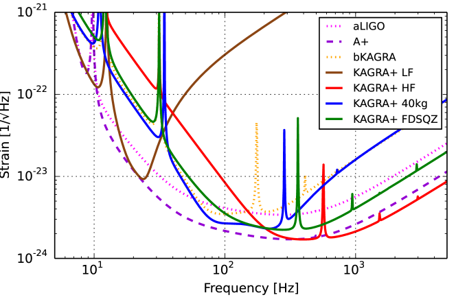
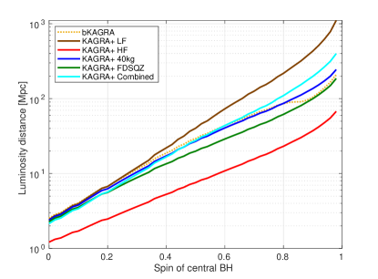
The current ground-based detectors, aLIGO and AdV, are planned to start upgrading their instruments around 2024 right after O4 observation ends and improve their sensitivities (called A+ A+ and AdV+ AdV+ , respectively) LVKScenario2018 . KAGRA KAGRA:NatureAstro will also be upgraded in the same term as aLIGO and AdV, though the concrete upgrade plan has not been decided officially yet. In this paper in a series of KAGRA-featured articles, we review scientific cases available with the second-generation ground-based detectors including aLIGO, AdV, the baseline KAGRA (bKAGRA) and their future upgrades, A+, AdV+, and KAGRA+, respectively, and discuss KAGRA’s scientific contributions to the global detector networks composed of the detectors above. Since the official design of KAGRA+ has not been decided yet, we consider four possible upgrade options for the near to middle term (5 years): one focused on low frequencies ( - ) [LF], one focused on high frequencies ( - ) [HF], to use heavier mirrors to improve middle frequencies ( - ) [40kg], and to inject frequency dependent squeezing for the broadband improvement [FDSQZ]222We divide frequencies into three ranges: low, middle, and high, depending on the shape of the noise curves in Fig. 1.. In addition to these, we also consider a slightly optimistic case in which technologies for four KAGRA+ upgrades are combined (called Combined). The noise curves of bKAGRA and its upgrade candidates are shown in Fig. 1. More details on the concrete plans and technological aspects are discussed in a companion paper in the series KAGRA:PTEP07 .
2 Stellar-mass binary black holes
2.1 Formation scenarios
- Scientific objective
The existence of massive stellar-mass BBH provides us a new insight about
formation pathways of such heavy compact binaries GW150914PRL ; GW151226PRL .
Since massive stars likely loose their masses by stellar winds driven by metal lines, dust, and pulsations
of the stellar surface, heavy BHs with masses of are not expected to be left as
remnants at the end of their lifetime of massive stars with metallicity of the solar value LIGO_ApJ .
In fact, the masses of BHs we have ever observed in EM waves (e.g., X-ray binaries) are
significantly lower than those detected in GWs GWTC1 .
This fact motivates us to explore the astrophysical origin of such massive stellar-mass BBH population
in low-metallicity environments
(below 50 % of solar metallicity or possibly less) LIGO_ApJ .
So far, a number of authors have proposed formation channels; evolution of low-metallicity isolated binaries
in the field Belczynski_2004 ; Dominik_2012 ; Belczynski_2016 ; Mapeli_2016 ,
dynamical processes in dense cluster systems (globular clusters, nuclear stellar cluster, or compact gaseous
disks in active galactic nuclei) Portegies Zwart_2000 ; O'Leary_2009 ; BaeKimLee ; Rodriguez_2016a ; Antonini_2016 ; Stone_2017 ; Park_2017 ,
massive stars formed in extremely low-metallicity gas at high-redshift Universe (Population III stars, hereafter Pop III stars)
Kinugawa_2014 ; Hartwig_2016 ; Inayoshi_2016 ; Inayoshi_2017 , and etc.
As an alternative non-astrophysical possibility, a primordial BH population in the extremely early universe (e.g., originated by phase transitions, a temporary softening in the EOS, quantum fluctuations) have been attracting attention Carr_2016 ; Sasaki_2016 (Sasaki:2018dmp for a review).
- Observations and measurements
In order to reveal the astrophysical origin of stellar-mass BBH detected by LIGO and Virgo, we need to explore the properties of coalescing BBH, depending on their formation pathway and environment where they form. In particular, the effective spin parameters of BBH (the dimensionless spin components aligned or anti-aligned with the orbital angular momentum) are expected to be useful to discriminate the evolution models Kushnir_2016 ; Rodriguez_2016b . In the field binary scenario, concerning binaries formed in a galactic plane, tidal torque exerting two stars (or one of them is a BH) in a close binary transport the orbital angular momentum into stellar spins, resulting in . Since tidal synchronization occurs as quickly as , a binary with a short GW coalescence timescale (i.e., a small orbital separation) would be significantly spun to . Since BBH populations formed at high redshift take a long GW coalescence timescale, their BBH are hardly affected by tidal torque Hotokezaka_Piran_2017 . The underlying assumption is that the orbital angular momentum is not significantly changed via natal kicks that new-born BHs could receive during the core collapse of their progenitors Janka_2013 . Although a strong natal kick is required to affect the effective spin parameter, observations of low-mass X-ray binaries show no evidence of such strong natal kicks of BHs (see, e.g., Mandel_2016 ).
On the other hand, in the dynamical formation scenario, concerning binaries formed in dense stellar environment, the distribution of effective spin would be isotropic at , and negative values are allowed unlike the isolated binary scenario because the directions of stellar spins could be chosen randomly. As a robust result of the formation channel, the effective spin can have negative values at . Moreover, in the dynamical capture model, a small fraction of the binaries/BBH could gain significantly high eccentricities (), which will be imprinted in the GW waveform O'Leary_2009 .
For PBHs formed in the early Universe (radiation dominated era), the spin is suppressed to Chiba:2017rvs or even smaller DeLuca:2019buf because they are formed from the collapses of density inhomogeneities right after the cosmological horizon entry. However, if the early matter phase exists after inflation, the spin can be large Harada:2017fjm . Because of the uncertainty in the early Universe scenario, it would be difficult to distinguish the PBH origin from the astrophysical ones.
In addition to the BBH population within a detection horizon of ,
BBH that coalesce at higher redshifts due to small initial separations are unresolved individually,
but contribute to a GW background (GWB).
The spectral shape of a GWB caused by compact binary mergers is characterized by a single-power law of
at lower frequencies (), is flattened from it at , and
has a cutoff at higher frequencies () Phinney_2001 .
Importantly, this result hardly depends on the merger history of the BBH population qualitatively.
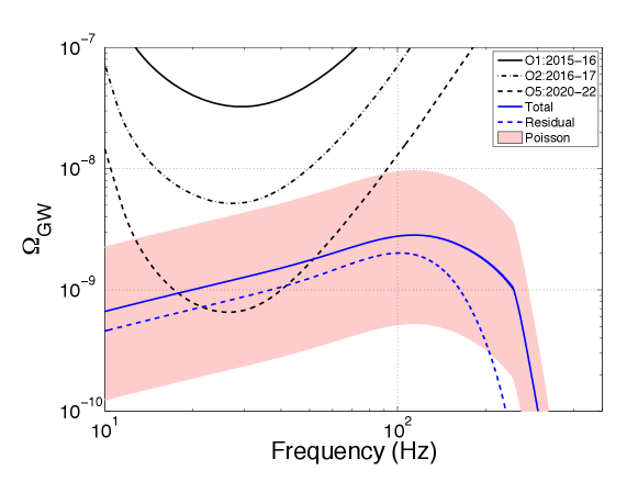
Therefore, a GWB produced from low-redshift, relatively less massive BBH population is robustly given by
in the frequency range. This GWB signal could be detected by future observing run O5 with aLIGO and AdV LIGO_background , as shown in Fig. 2.
In fact, the spectral flattening occurs outside the GWB sensitive frequency range ().
On the other hand, a GWB caused by merger events of higher redshift, massive BBH population suggested by Pop III models are expected to be flattened at a lower frequency of Inayoshi_2016 ,
where LIGO/Virgo/KAGRA are the most sensitive.
A detection of the unique flattening at such low frequencies will indicate the existence of a high-chirp mass,
high-redshift BBH population, which is consistent with the Pop III origin.
The detailed study of the GWB would enable us to explore the properties of massive binary stars at higher
redshift and the epoch of cosmic reionization.
- Future prospects
LIGO-Virgo’s sensitivities during O1 and O2 have been proved to be efficient to detect stellar-mass BBH with a mass range between (1-100) (GWTC1, ). The typical detection frequency of these stellar-mass BBH are between 30-500 Hz. The bKAGRA’s sensitivity would be similar to aLIGO and AdV and we expect the observable sample for bKAGRA would be similar to those listed in GWTC-1 (GWTC1, ), i.e., stellar-mass BBH. The LIGO-Virgo-KAGRA (LVK) configuration would provide a better sky localization but without finding a host galaxy (via EM waves), it would be challenging to identify the location of a BBH (in a galactic disk or in a cluster, for example).
Toward the upgrades of bKAGRA, we expect the improved sensitivity toward the lower frequencies would be useful to increase the signal-to-noise ratio (SNR) for BBH populations. More observation means better number statistics in event rate estimation and distributions for underlying properties such as BH mass distribution. Furthermore, by observing earlier inspiral phase signals available at lower frequencies, it will be possible to achieve better accuracy in parameter estimation for individual masses and spin parameters. For a BBH population with small masses, say total mass below 10 , by improving the so-called ‘bucket’ sensitivity around a few hundred Hz would be most effective to increase the detectability as well as the precision of parameter estimation.
From the stellar-mass to supermassive populations, BHs are considered to have a broad mass spectrum. While a standard binary evolution scenario prefers a compact binary consisting of similar masses PostnovYungenson , some binaries may have mass ratio much larger than 1, where is the primary mass and is the secondary mass of the binary. Dense stellar system is considered to be a factory to generate compact binaries through dynamical interactions, e.g. Benacquista . However, a toy model for the dynamic formation scenario for compact binaries still prefers BBH with , e.g. BaeKimLee . Unequal-mass BBH with a few are in particular interesting as the modulations in amplitude that is expected by post-Newtonian formalism in the inspiral phase become significant. Higher multiple modes (with the existence of spin(s)) are also more important for binaries with large mass ratios than equal-mass binaries Pekowsky_2013 . Therefore, detections of unequal-mass binaries require the overall improvement in the detector sensitivity corresponding to the detection frequency band in the ‘bucket.’ Indeed, the recent event, GW190412, has provided us the evidence to support the detection of the higher multiple models and proved that a broader frequency band play a crucial role for the detection LIGOScientific:2020stg .
In Table 1, we present the innermost stable circular orbit (ISCO) frequencies Bardeen:1972fi corresponding to stellar-mass BBH or BH-NS binaries with various masses. GW signals from binaries with the total mass of (10) M⊙ or larger would be spanned between of an interferometer and around the estimated assuming the duration of ringdown signals would be much shorter than inspiral signals. The actual detectability will depend on the sensitivity of the interferometer within the frequency range given the binary.
| () | () | () | () | (Hz) |
| 1.4 | 1.4 | 2.8 | 1 | 1574 |
| 5 | 1.4 | 6.4 | 3.6 | 1001 |
| 10 | 1.4 | 11.4 | 7.1 | 387 |
| 10 | 10 | 20 | 1 | 220 |
| 30 | 10 | 40 | 3 | 110 |
| 40 | 30 | 70 | 1.3 | 63 |
In Table 2 and 3, the measurement errors of the binary parameters for equal-mass BBH with and at are estimated with the Fisher information matrix. We assume the detector networks composed of A+, AdV+, and bKAGRA or KAGRA+ (LF, HF, , FDSQZ, or combined). The waveforms we use are the spin-aligned inspiral-merger-ringdown waveform (PhenomD) for BBH. There are significant improvements from 2G detectors to 2.5G detectors (bKAGRA, LF, HF, 40kg, FDSQZ, Combined) in the SNR and the errors. But this is not solely due to KAGRA’s contribution. The upgrade of bKAGRA to KAGRA+ among A+ and AdV+ modestly enhances the SNR and the sensitivities to the binary parameters in GW phase: the symmetric mass ratio , the effective spin , and the luminosity distance to a source . For the parameters in GW amplitude, the orbital inclination angle and the sky localization area , the improvement of the errors is significant because the fourth detector is important to pin down the source direction and determine the other correlated parameters. The improvement factor depends on the configuration of the upgrade of KAGRA+. From the point of view to discriminate the formation scenarios, it would be better for KAGRA to improve the detector sensitivity at both low and middle frequencies. In addition, in order to increase the detectability of BBH coalescences at higher redshifts such as Pop III star binaries and primordial BH binaries, it is important to increase the horizon distance for BBH and analyze together with the data of a GWB measuring the spectral index and the spectral cutoff.
| quantities | 2G | bKAGRA | LF | HF | 40kg | FDSQZ | Combined |
|---|---|---|---|---|---|---|---|
| SNR | 44.4 | 76.4 | 75.5 | 76.0 | 81.2 | 81.5 | 89.5 |
| 9.13 | 5.62 | 5.83 | 5.60 | 5.15 | 5.23 | 4.61 | |
| 15.6 | 9.75 | 9.41 | 9.58 | 9.35 | 9.13 | 8.59 | |
| 11.7 | 6.82 | 8.67 | 7.19 | 6.19 | 7.32 | 5.79 | |
| 8.89 | 4.92 | 6.35 | 5.60 | 4.68 | 5.25 | 4.36 | |
| 0.805 | 0.300 | 0.648 | 0.263 | 0.243 | 0.219 | 0.169 |
| quantities | 2G | bKAGRA | LF | HF | 40kg | FDSQZ | Combined |
|---|---|---|---|---|---|---|---|
| SNR | 19.8 | 32.4 | 31.6 | 34.2 | 34.9 | 33.9 | 36.7 |
| 24.2 | 14.9 | 15.2 | 13.2 | 13.9 | 13.7 | 12.6 | |
| 9.48 | 6.02 | 5.73 | 5.83 | 5.75 | 5.87 | 5.62 | |
| 25.0 | 15.0 | 19.8 | 15.6 | 14.2 | 13.9 | 11.8 | |
| 19.1 | 10.7 | 13.7 | 12.5 | 10.8 | 10.1 | 8.55 | |
| 1.96 | 0.821 | 1.44 | 0.404 | 0.654 | 0.487 | 0.451 |
3 Intermediate-mass binary black holes
3.1 Formation scenarios
- Scientific objective
The direct detections of GW emission have revealed the existence of massive BHs with masses of , which are significantly heavier than those ever observed in X-ray binaries
GW150914PRL ; LIGO_ApJ ; GWTC1 .
On the other side, supermassive BHs with the order of almost ubiquitously exist
at the centers of galaxies and are believed to be one of the most essential components of galaxies.
However, the existence of a (binary) BH population between stellar-mass and supermassive regime,
i.e., , has not been confirmed yet (though there are some candidates).
The lack of such intermediate-mass binary BH (IMBBH) population is one of the most intriguing unsolved puzzles in astrophysics.
Detection of GWs from IMBBH would be one of the best way to probe their existence and physical natures.
- Observations and measurements
A plausible formation pathway of IMBHs is runaway collisions of massive stars in dense stellar systems (e.g., globular clusters and/or nuclear stellar clusters) Portegies_Zwart_2002 ; Freitag_2006 . In a dense young star cluster, massive stars sink down to the center due to mass segregation and begin to physically collide. During the collision processes, the most massive one gains more masses and grow to a very massive star (VMS) in a runaway fashion, and thus an IMBH with a mass of is left after gravitational collapse of the VMS. Even after IMBH formation, stellar-mass BHs (SBHs) are migrating to the central region and could form a binary system with the IMBH, which is so-called intermediate-mass ratio inspirals (IMRIs) Amaro-Seoane_2010 ; Fragione_2018 . GW emission from such IMRI systems can be detected not only by space-borne GW observatories such as LISA but also by ground-based detectors whose configurations are specifically designed to reach a better sensitivity at lower frequencies (e.g., A+ or KAGRA LF). For and , GWs produced from the IMRIs can be detected up to a distance of a few Gpc Shinkai_2017 . Since IMRIs systems are likely to have high eccentricities due to the formation process, the GW energy distribution is shifted to higher frequencies, increasing the SNR Amaro-Seoane_2018 . Although the IMRI coalescence rate is still highly uncertain, events yr-1 would be expected from several theoretical studies Shinkai_2017 ; Fragione_2018 . In addition, Gurkan_2006 discussed the possibility that two IMBHs are formed in a massive dense cluster via runaway stellar collisions, and would form an IMBBH at a lower rate Amaro-Seoane_2010 .
Alternatively, formation of VMSs in extremely low-metallicity environments (Pop III stars)
can initiate IMBHs with masses of Hirano_2014 .
Since a molecular cloud forming massive Pop III stars would be very unstable against its self-gravity,
the cloud would be likely to fragment into massive clumps with and leave
a very massive binary system that will collapse into IMBBH with Stacy_Bromm_2013 ; Susa_2014 ; Inayoshi_Haiman_2014 .
Assuming a Salpeter-like initial stellar mass function and the merger delay-time distribution to be ,
the merger event rate for such IMBBH is inferred as , and thus a few events yr-1 Kinugawa_2014 .
- Future prospects
The possible target source that is detectable with ground-based detectors is IMRIs. See the next section 3.2.
3.2 Intermediate mass-ratio binaries
- Scientific objective
The existence of IMBHs in globular clusters is suggested both by observational evidence and theoretical prediction Miller:2003sc . An IMBH in a globular cluster may capture a stellar-mass compact object surrounding it through some process (e.g. two-body relaxation), and may form an intermediate mass-ratio binaries (IMRB) (where “intermediate” mass-ratio means the range between the comparable mass ratio () and extreme-mass ratio ()).
The captured object in an IMBR orbits the IMBH many times during the
inspiral phase before it plunges into the BH. Therefore,
GW signals from IMRBs contain information on the
geometry around the IMBHs, which can be used to test the general
relativity in the strong field, for example, the
no-hair theorem of BHs and the tidal coupling between the central BH
and the orbit of the captured object Brown:2006pj .
Also, if the observation of IMRBs are accumulated, it may give
a constraint on the event rate and population of IMBHs.
- Observations and measurements
The GW waveform from the inspiral phase of an IMRB can be estimated in the stationary phase approximation by
| (1) |
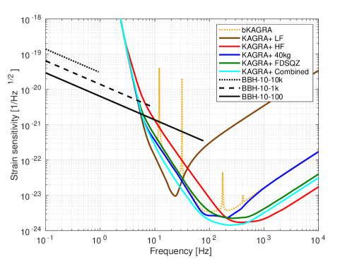
where , and are the redshifted chirp mass of the binary, the luminosity distance to the source, and the GW phase, respectively Berti:2004bd ; Isoyama:2018rjb . The black (solid, dash, dot) lines in Fig.3 show the strain amplitude of GWs, , from IMBRs for three different cases, in which a BH with spirals into heavier BHs with masses of , , and (these masses include the redshift factors) and the same spin parameter of at the luminosity distance of 100 Mpc.
The inspiral phase ceases around certain cutoff frequency, which corresponds to the frequency just before the plunge phase. For circular orbit cases, the cutoff is estimated by the frequency for an ISCO Bardeen:1972fi . The ISCO frequency, mainly depends on the mass and spin of the central BH. If the mass decreases or the spin increases, the ISCO frequency becomes higher and the overlap with the sensitive band of ground-based detectors becomes larger.
After the inspiral phase, the orbit of the captured object changes
to the plunge phase through the transition phase. The shift of the
frequency during the transition is roughly estimated by
, where is the mass
ratio Ori:2000zn . The plunge of the object to the
central IMBH will induce ringdown GWs, whose frequency of the
dominant mode is given by
,
where and are the redshifted mass and spin of the IMBH
and shows the spin dependence (see Ref.Berti:2005ys
for details).
Since the contribution from the transition phase and the ringdown
phase is smaller than that from the inspiral phase, here we do not
consider them (An analysis including the transition and ringdown
is shown in Huerta:2010un ).
- Future prospects
Since IMRBs with the redshifted mass of - are expected to be GW sources in Hz band Miller:2008fi , some of them may be possible targets for the low frequency band of ground-based detectors. To see the dependence of the detectability on the sensitivity in lower band, here we consider the detectable luminosity distance for the design sensitivity of the bKAGRA and KAGRA+ in the same way in Isoyama:2018rjb .
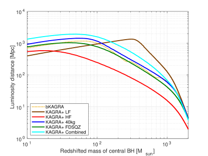
The left panel in Fig.4 shows the dependence of
on the redshifted mass of the central IMBH
() with fixed spin parameter ().
The right panel shows the dependence of on
the spin parameter with fixed mass ().
In both figures, we fix the mass () and spin parameter
() of the captured object, and the threshold of .
For example, the values of with
,
and SNR are given as
62, 126, 16, 59, 42, 67 Mpc for bKAGRA, LF, HF, 40kg, FDSQZ, and Combined, respectively.
From the figures, we find that the detectability of IMBRs with
can be improved significantly by the LF,
while it is difficult to detect IMBRs by the HF.
To detect an event, the detection volume is a crucial quantity because it is roughly proportional to the event rate.
Using the detector network composed of two A+, AdV+, and bKAGRA or
KAGRA+ (LF, HF, 40kg, FDSQZ, and Combined),
the improvement factors of the detection volume are LF 8.29, 40kg 0.85, FDSQZ 0.30, HF 0.02, Combined 1.27
for - BBH with spin 0.7.
4 Neutron star Binaries
4.1 Binary evolution
- Scientific objective
Formation scenarios of BNS are similar to those of stellar-mass BBH. One is based on the standard binary evolution in a galactic disk (e.g., Tauris:2017 ; Chruslinska:2018 ) and the other involves dynamical interactions in dense stellar environments such as globular clusters (e.g., Pooley:2003 ). By precision measurements of the NS masses and orbital parameters such as eccentricity by GW observations, it would be possible to shed lights on the origin of the BNS formation as pointed out many previous works on the BNS population including Tauris:2017 . Although the expected kick involved in the BNS formation is small Tauris:2017 , the role of the natal kick from a supernova explosion can be relatively more significant for the BNS formation than that of BBH formation. The evidence of the natal kick is observed in the known BNS in our Galaxy, such as the Hulse-Taylor binary pulsar where the eccentricity is 0.67 WeisbergNiceTaylor . Even though a binary’s orbit could be significantly eccentric at the time of formation, the BNS orbit becomes circularized quite efficiently Peters and typical BNS within the detection frequency band of KAGRA is expected to have an eccentricity below . Similar to BBH, if there are eccentric NS binaries within the KAGRA frequency band, they are more likely to be formed through stellar interactions in dense stellar environment BaeKimLee ; Rodriguez_2016a . If eccentric binaries exist, measuring eccentricity would be one useful probe to distinguish the field population (formed by a standard binary evolution scenario) and the cluster population (formed by stellar interactions). We note that the measurement of eccentricity requires a much better sensitivity toward the lower frequency band below 20 Hz, therefore it is more plausible that a third generation detector may be better suited for searching eccentric BNSs.
Another difference between NS and BH populations is the mass range. While BH mass spectrum spans over nine orders of magnitudes, the NS mass range is narrow. For example, the NS mass range should depend on the formation mechanism but is estimated, assuming the Gaussian distribution, to be for double NSs, for recycled NSs, and for slow pulsars, which are likely to be NSs right after their birth ozelFreire:2016 . These are based on the known NS-pulsar binaries in our Galaxy before 2016 and do not include a possibly heavy NS recently discovered by GWs Abbott:2020khf , but even if included, the mass range of NSs is much narrower than that of BHs, which is advantageous of establishing a template bank. In addition, spin distribution would be something to be compared between NS and BH populations. NS spin distribution for those in BNS is not well constrained and we expect GW observations would shed light on the NS spin distribution by parameter estimation.
- Observations and measurements
As of early 2019, there are fifteen BNS known in the Galactic disk (e.g., see Table 1 in (PML2019, )), where all systems consisting of at least one active radio pulsar ATNFPulsarCatalogue . Eight of them are expected to merge within a Hubble time. Measurements of binary’s orbital decay and other post-Keplerian parameters clearly showed the effects of gravitational radiation in these NS-pulsar binaries.
GW170817 is the first BNS discovered by GW observation. It is also the first extragalactic BNS. The binary is identified as BNS based on the mass estimation, where both and estimates are consistent with expected NS masses Abbott:2018wiz . The detection of GW170817 also makes it possible to constrain the BNS merger rate. Considering the first and second observing runs, the merger rate solely based on GW observation is estimated to be 110 - 3840 at 90% confidence interval GWTC1 . GW observation can observe extragalactic BNS, which are not accessible with current radio telescopes. The GW and radio observation of BNS would be complimentary to reveal underlying properties of the BNS.
In addition to the BNS population, GW observation would be able to provide rich information about neutron star interior (see Secs. 4.2 and 4.3) or the formation of young NSs (see also Secs. 6.3 and 7.1) if late-inspiral, merger, or even ringdown phases are observed by future detectors.
- Future prospects
In terms of an observation, improving sensitivities toward lower and higher frequencies have significant implications for understanding astrophysics of BNS. A typical chirp mass of a BNS is assuming . This implies the frequencies of merger and ringdown phases would be around 2 kHz where the current generation of GW detectors are not sensitive. However, the merger and ringdown phases of BNS coalescence would provide crucial hints on the remnant of the merger. On the other hand, the lower cutoff frequency of a detector is crucial to measure the early inspiral phase.
Effects of improved sensitivity of a detector can be considered in two folds: (a) At higher frequencies, better sensitivity would allows us to put stronger constrains for the NS EOS than what aLIGO and AdV could do for GW170817 Abbott:2018exr , not to mention improving accuracy for mass and spin parameters at higher post-Newetonian (PN) orders. Therefore, better sensitivities in high frequencies will be useful to have the observed sample of BNS via GWs as complete as possible in the mass-spin parameter space. (b) Improved sensitivity toward the lower frequencies below 20 Hz allows us observing early-inspiral signals. This would be crucial to constrain the orbital eccentricity and determine the origin of the binary formation.
BH-NS binaries are expected to exist and their evolution would be similar to those of stellar-mass BBH and BNS. As mentioned above, as there are several parameters necessary to be measured in order to discriminate the formation scenarios, we estimate with the Fisher information matrix the measurement errors of the binary parameters for a BH-NS binary is at and a BNS at . The waveform we use is the spin-aligned inspiral waveform up to 3.5PN in phase. The maximum frequency for the inspiral part is set to the ISCO frequency. We assume the detector networks composed of A+, AdV+, and bKAGRA or KAGRA+ (LF, HF, , FDSQZ, or combined). The measurement errors of the binary parameters are shown in Table 4 and 5. There are significant improvements from 2G detectors to 2.5G detectors (bKAGRA, LF, HF, 40kg, FDSQZ, Combined). But this is not solely due to KAGRA’s contribution. The upgrade of bKAGRA to KAGRA+ among A+ and AdV+ modestly enhances the SNR and the sensitivities to the binary parameters in GW phase: the symmetric mass ratio , the effective spin , and the luminosity distance to a source . For the parameters in GW amplitude, the orbital inclination angle and the sky localization area , the improvement of the errors is significant because the fourth detector is important to pin down the source direction and determine the other correlated parameters. The improvement factor depends on the configuration of the upgrade of KAGRA+. From the point of view to discriminate the formation scenarios, it would be better for KAGRA to improve the detector sensitivity at both low and middle frequencies.
| quantities | 2G | bKAGRA | LF | HF | 40kg | FDSQZ | Combined |
|---|---|---|---|---|---|---|---|
| SNR | 13.8 | 22.3 | 21.9 | 22.3 | 23.6 | 22.6 | 25.4 |
| 9.47 | 8.93 | 8.86 | 8.86 | 8.86 | 8.87 | 8.71 | |
| 98.2 | 80.9 | 80.5 | 78.2 | 78.7 | 78.6 | 73.3 | |
| 42.6 | 24.6 | 27.0 | 26.7 | 22.0 | 22.8 | 20.8 | |
| 32.2 | 19.6 | 20.8 | 21.5 | 16.8 | 16.4 | 15.0 | |
| 9.04 | 4.26 | 9.02 | 3.48 | 3.57 | 3.42 | 2.71 |
| quantities | 2G | bKAGRA | LF | HF | 40kg | FDSQZ | Combined |
|---|---|---|---|---|---|---|---|
| SNR | 14.8 | 22.9 | 23.6 | 24.1 | 24.5 | 24.3 | 27.7 |
| 8.50 | 5.91 | 5.48 | 5.64 | 5.76 | 5.74 | 5.18 | |
| 5.65 | 3.96 | 3.67 | 3.79 | 3.87 | 3.87 | 3.49 | |
| 37.1 | 21.5 | 26.4 | 21.4 | 18.6 | 18.7 | 17.4 | |
| 30.1 | 15.2 | 18.2 | 17.1 | 14.3 | 13.7 | 13.8 | |
| 3.14 | 1.60 | 2.39 | 0.80 | 1.28 | 1.05 | 0.790 |
4.2 Neutron star equation of state and tidal deformation
- Scientific objective
BNS mergers provide us rich information to study nuclear astrophysics.
Since NSs consist of ultra-dense matter Lattimer:2015nhk .
In the BNS system, a NS is deformed by the tidal field generated by the companion star in the late-inspiral stage
Flanagan:2007ix ; Hinderer:2007mb ; Damour:2012yf .
The tidal deformability originating from the matter effect encodes the information of NS EOS.
Therefore, the measurement of the tidal deformabilities from GWs of the BNS mergers provides the information about nuclear physics
Wade:2014vqa ; Hinderer:2009ca ; Hotokezaka:2011dh . In this section, we investigate the ability to measure the tidal deformability of NSs with current and future detector networks including bKAGRA and KAGRA+ in addition to the A+ and AdV+.
- Observations and measurements
During the late stages of the BNS inspiral, at the leading order, the induced quadrupole moment tensor is proportional to the external tidal field tensor as . The information about the NS EOS can be quantified by the tidal deformability parameter , where is the second Love number and is the stellar radius Flanagan:2007ix ; Hinderer:2007mb . The leading-order tidal contribution to the GW phase evolution appears through the binary tidal deformability Wade:2014vqa
| (2) |
which is a mass-weighted linear combination of the both component tidal parameters, where is the dimensionless tidal deformability parameter . It is first imprinted at relative 5PN order.
The first detection of a GW signal from a BNS system, GW170817 GW170817PRL ,
provides an opportunity to extract information about NSs via measuring the tidal deformability.
The LIGO-Virgo collaboration has placed an upper bound on the tidal deformability as
when restricting the magnitude of the component spins GW170817PRL
using the restricted TF2 model Buonanno:2009zt ; Blanchet:2013haa
(this limit is later corrected to be in Ref. Abbott:2018wiz ).
In Ref. Abbott:2018wiz ; GWTC1 , the updated analysis by the LIGO-Virgo collaboration by using a numerical-relativity (NR) calibrated waveform model,
NRTidal Dietrich:2017aum have been reported.
By using EOS-insensitive relations among several properties of NSs Yagi:2016bkt ,
the constraints on can be improved Abbott:2018exr
(but see also Kastaun:2019bxo ).
As found in Refs. Abbott:2018wiz ; LIGOScientific:2019eut , the stiffer EOSs (large radii)
yielding larger tidal deformabilities such as MS1 and MS1b Mueller:1996pm
are disfavored by the data of GW170817.
Independent analyses have also been done
by assuming the common EOS for both NSs De:2018uhw ; Capano:2019eae .
In Ref. Narikawa:2019xng , the authors indicate that there is a difference in estimates of
for GW170817 between NR calibrated waveform models (the KyotoTidal and NRTidalv2 models).
Here, the KyotoTidal model is one of NR calibrated waveform models of inspiraling BNS
Kiuchi:2017pte ; Kawaguchi:2018gvj and NRTidalv2 model is an upgrade of the NRTidal model Dietrich:2019kaq .
Several other studies have also derived constraints on the NS EOS via measuring tidal deformability from GW170817 Margalit:2017dij ; Bauswein:2017vtn ; Ruiz:2017due ; Annala:2017llu ; Zhou:2017pha ; Fattoyev:2017jql ; Paschalidis:2017qmb ; Nandi:2017rhy ; Most:2018hfd ; Raithel:2018ncd ; Landry:2018prl . A review of these and other results are available in Baiotti:2019sew .
- Future prospects
In order to investigate the expected error in the measurement , we use the Fisher matrix analysis with respect to the source parameters , where is the luminosity distance, and are the time and phase at coalescence, is the chirp mass, and is the symmetric mass ratio. We use the restricted TF2_PNTidal model, which employ the 3.5PN-order formula for the phase and only the Newtonian-order evolution for the amplitude as the point-particle part Buonanno:2009zt ; Blanchet:2013haa and the 1PN-order (relative 5+1PN-order) tidal-part phase formula (see e.g., Damour:2012yf ). We take the frequency range from 23 Hz to the ISCO frequency. Here, we consider non-spinning binary for simplicity.
In Table 6, we show the fractional errors in the tidal deformability in the cases of some NS EOS models, using the inspiral PN waveform, the TF2_PNTidal model. We assume future detector networks including bKAGRA and KAGRA+ in addition to two A+ and AdV+. We assume 1.35-1.35 BNS located at a distance of 100 Mpc and study three different NS EOS models Takami:2014tva : APR4 Akmal:1998cf (=321.7), SLy Douchin:2001sv (=390.2), and high- (=1000). In one example, for the SLy, the fractional error on the tidal deformability are 0.069, 0.070, 0.061, 0.068, 0.067, and 0.062 for bKAGRA, LF, HF, 40kg, FDSQZ, and Combined, respectively. We find that the measurement precision of the tidal deformability can be slightly improved for the HF, while cannot be done for the LF. We also present the fractional errors in the tidal deformability for the single detector case in Table 7 to see how much KAGRA can contribute to the global networks.
In Ref. Narikawa:2018yzt , the authors have found a discrepancy in the tidal deformability of GW170817 between Hanford and Livingston detectors of aLIGO. While the two distributions look consistent with each other and also consistent with what we would expect from noise realization, the Livingston data are not very useful to determine the tidal deformability for GW170817. Their results suggest that the measurement of the tidal deformability by the third detector such as AdV or bKAGRA might be helpful in order to improve the constraint on the tidal deformability. In Ref. Narikawa:2019xng , their results indicate that the systematic error for the NR calibrated waveform models will be significant to measure from upcoming GW detections. It is needed to improve current waveform models for the BNS mergers.
| bKAGRA | LF | HF | 40kg | FDSQZ | Combined | |
| APR4 () | 0.834 | 0.0840 | 0.0735 | 0.0826 | 0.0795 | 0.0750 |
| SLy () | 0.0689 | 0.0695 | 0.0608 | 0.0683 | 0.0658 | 0.0620 |
| High- () | 0.0276 | 0.0278 | 0.0244 | 0.0273 | 0.0263 | 0.0248 |
| Network SNR | 105 | 102 | 105 | 108 | 106 | 115 |
| Source | aLIGO | bKAGRA | LF | HF | 40kg | FDSQZ | Combined |
|---|---|---|---|---|---|---|---|
| APR4 () | 0.289 | 0.659 | 59.7 | 0.231 | 0.589 | 0.270 | 0.180 |
| SLy () | 0.239 | 0.545 | 49.3 | 0.192 | 0.487 | 0.223 | 0.149 |
| High- () | 0.0939 | 0.217 | 19.3 | 0.796 | 0.194 | 0.0903 | 0.0598 |
| SNR | 33.9 | 26.7 | 12.4 | 27.4 | 35.4 | 31.4 | 53.9 |
4.3 Neutron star remnants
- Scientific objective
Investigating the evolution of the object that forms after the merger of a BNS system is more difficult, but also, possibly, rewarding (see bai17 ; Duez2019 ; Baiotti:2019sew for recent reviews). In addition to the connection between such a merged object and ejecta powering the kilonova (which will be treated in detail in Sec. 11.1), strong interest in observations of the post-merger phase comes also from the fact that these would at some point yield information about the EOS of matter at densities higher (several times the nuclear density) than typical densities in inspiralling stars and also at much higher temperatures (up to MeV).
Interestingly, the post-merger phase may be luminous in GW emission, perhaps more so than the preceding merger phase, but, since post-merger GW frequencies are higher (from 1 to several kHz [116, 118]), the SNR for current and projected detectors is smaller than the pre-merger phase. However, when analyzed in different ways, such GW emission gives us a novel opportunity to prove for a hypermassive NS (HMNS) in the immediate post-merger phase (see below in this subsection). Also gravitational collapse to a rotating BH, should it occur, opens an additional window to emission from a BH-torus system at relatively lower frequencies (van19b, ).
Theoretical estimates from numerical simulations of emission from the post-merger HMNS are less reliable than those of the inspiral, because such simulations are intrinsically more difficult to carry out accurately. This is due to the presence of strong shocks, turbulence, large magnetic fields, various physical instabilities, neutrino cooling, viscosity and other microphysical effects. Currently there exist no reliable determinations of the phase of post-merger gravitational radiation, but only of its spectrum (see, e.g., Takami:2014zpa ; Maione2017 ; Paschalidis_and_Stergioulas_2017 ; Breschi2019 ).
Measuring even just the main frequencies of the post-merger waveform from the putative HMNS may, however, give precious hints on the supranuclear EOS. It has been found, in fact, that the frequencies of the main peaks of the post-merger power spectrum strongly correlate with properties (radius at a fiducial mass, compactness, tidal deformability, etc.) of a zero-temperature spherical equilibrium star (see, among others, Bauswein2011 ; Takami:2014zpa ; Maione2017 ; Paschalidis_and_Stergioulas_2017 and, for applications, Bose2017 ; Chatziioannou2017 ; Torres-Rivas2019 ; Breschi2019 ). For example, finding the tidal deformability of the post-merger object to be very different from that estimated from the inspiral may hint at phase transitions in the high-density matter (see Baiotti:2019sew for a review). A similar hint would be given by an abrupt change in the post-merger main frequency Weih2020 ; Bauswein2020 . The complicated morphology of these post-merger signals makes constructing accurate templates challenging and thus matched-filtering less efficient Breschi2019 .
In addition to predictions on the GW spectrum, simulations also show, in most cases, delayed gravitational collapses to a rotating BH with dimensionless spin parameter (bai08, ), surrounded by a disc. Strong magnetic fields (rez11, ) and baryon-rich disk winds are also predicted, though with inferior accuracy, and they are prescient to kilonova light curves (kiu15, ).
However, simulations cannot accurately predict the time of delay in gravitational collapse of the putative HMNS to a BH, representative for the lifetime of the HMNS initially supported against collapse by differential rotation. The lifetime of the HMNS may be measured in EM-GW observations. Furthermore, because of constraints in computational resources, simulations of post-merger BH-disk or torus systems are limited to tens of ms (e.g. bai17, ; rad18, ). Yet, rotating BHs provide a window to powerful emission over a secular Kelvin-Helmholtz time-scale , where is the spin-energy in angular momentum of a Kerr BH of mass (ker63, ), is the velocity of light and is the total BH luminosity most of which may be irradiating surrounding matter (van99, ). For gamma-ray bursts, canonical estimates show to be tens of seconds (van19b, ).
EM-GW observations promise to fill the missing links in our picture of BNS mergers, namely the lifetime of the HMNS in delayed gravitational collapse to a BH (e.g. dep19a, ; kli19, ). If finite, continuing emission may extend over the lifetime of BH spin by above. For GW170817, if the HMNS experienced delayed collapse, the merger sequence
| (3) |
offers a unique window to post-merger EM-GW emission powered by the energy reservoir of the remnant compact object. Crucially, gravitational collapse to a BH in the process (3) can increase significantly above canonical bounds on the same at formation of the progenitor HMNS (hae09, ) in the immediate aftermath of the merger.
In the following subsection, we will focus only on calorimetric studies of the
post-merger object, leaving the other topics to the above-mentioned
reviews bai17 ; Duez2019 ; Baiotti:2019sew .
- Observations and measurements
Post-merger EM-calorimetry on GRB170817A and the kilonova AT 2017gfo con17 ; sav17 ; moo18a ; moo18b show a combined post-merger energy in EM radiation limited to . This output is well-below the scale of total energy output in GW170817, and is insufficient to break the degeneracy between a HMNS or BH remnant.
Gravitational radiation provides a radically new opportunity to probe a transient source which, “if detected, promises to reveal the physical nature of the trigger” cut02 . GW-calorimetry builds on earlier applications of indirect calorimetry to, notably, PSR1913+105 hul75 and pulsar wind nebulae wei78 . Power-excess methods GW170817:GRB ; abb19a have thus far proven ineffective, however, by a threshold of sun19 , given a total mass of the BNS progenitor and hence the mass of its remnant compact object.
Independent EM and GW observations corroborate the process (3) with a lifetime of the HMNS of less than about one second (van19b, ; gil19, ). In EM, the lifetime of the HMNS is inferred from an initially blue component in the kilonova AT 2017gfo sma17 ; pia17 ; rad18 ; poo18 ; gil19 ; luc19 , whereas the same is inferred from the time-of-onset of post-merger GW-emission in time-frequency spectrograms produced by butterfly filtering, developed originally to identify broadband Kolmogorov spectra of light curves of long GRBs in the BeppoSAX catalogue van14 ; van17 . Application to the LIGO snippet of 2048 s of H1-L1 O2 data covering GW170817 serendipitously shows observational evidence of s post-merger gravitational radiation van19a . Subsequent signal injection experiments indicate an output in this extended emission (van19b, ). Its time-of-onset s post-merger falls in the 1.7 s gap between GW170817 and GRB170817A, satisfying causality at birth of a central engine of GRB170817A.
exceeds the maximal spin-energy of a (HM)NS hae09 , yet it readily derives from of a BH following gravitational collapse thereof at in the process (3). Moreover, aforementioned is quantitatively consistent with model predictions of ultra-relativistic baryon-poor jets and baryon-rich disk winds from a BH-torus system, the size of which derives from the frequency of its gravitational-wave emission van19b .
At current detector sensitivities, witnessing the formation and evolution of the progenitor HMNS in the immediate aftermath of a merger is extremely challenging. Null-results on GW170817 (GW170817:PMS, )
are entirely consistent with the energetically moderate and relatively high-frequency (kHz) spectra expected from numerical simulations (bai17, ).
- Future prospects
Once the BH forms, it has no memory of its progenitor except for total mass and angular momentum. This suggests pursuing GW-calorimetry in (3) to catastrophic events more generally, including mergers of a NS with a BH companion and nearby core-collapse supernovae (CCSNe), notably the progenitors of type Ib/c of long gamma-ray bursts (GRBs) van19c . While the latter is rare, the fraction of failed GRB-supernovae that are nevertheless luminous in gravitational radiation may exceed the local GRB rate and hence the rate of mergers involving a NS (e.g. van14, ). Blind all-sky butterfly searches may thus produce candidate signals with and without merger precursors from events within distances on par with GW170817, that may be followed up by time-slide correlation analysis and optical-radio signals from existing transient surveys of the local Universe. It also appears opportune to consider directed searches for events in neighboring galaxies (e.g. heo16, ), notably M51 (Mpc) and M82 (Mpc) each offering about one radio-loud CCSN per decade. By their close proximity, such appears of interest also independent of any association with progenitors of GRBs (and13, ; aas14, ).
For a planned KAGRA upgrade, the above suggests optimizing the broadband window of 50-1000 Hz to pursue GW-calorimetry on extreme transient sources using modern heterogeneous computing, in multi-messenger approaches involving existing and planned high-energy missions such as THESUES ama18a ; stra18a .
Jointly with LIGO and Virgo, KAGRA is expected to give us a window to modeled and unmodeled transient events out to tens of Mpc.
5 Accreting binaries
5.1 Continuous GWs from X-ray binaries
- Scientific objective
There are several classes of continuous GWs (CWs). One major population of CW sources is systems involving a spinning NS that has an asymmetry with respect to its rotation axis Riles2017 . Potential candidates include pulsars, NSs in supernova remnants, and NSs in binary systems. In particular, an accreting NS in a low-mass X-ray binary is a promising target. In this system, the central NS accretes materials from an orbiting late-type companion star. Finite quadrupole moment of an accreting NS can be possibly induced by various processes such as the laterally asymmetric distribution of accreted material, elastic strain in the crust as well as magnetic deformation Ushomirsky2000 .
Sco X–1 is the prime target for directed searches of CWs from X-ray binaries because it is the brightest persistent X-ray binary. The source is relatively nearby ( kpc) and its X-ray luminosity suggests that the source is accreting near the Eddington limit for a NS. If the torque-balance (i.e. balance between accretion-induced spin-up torque and the total spin-down torque due to gravitational and EM radiation) can be maintained in the binary system, Sco X–1 is a promising target for CW signals Bildsten .
Theoretical understanding of torque-balance and spin wandering effects of X-ray binaries are poorly understood Bildsten ; Mukherjee2018 . By combining CWs from X-ray binaries and multi-wavelength observations, we may track the evolution of spin torques and orbit, shedding light on disk dynamics and maximum rotation frequency of a NS in a binary system Riles2017 .
No CW signal from X-ray binaries has been observed so far. During LIGO S6, upper limits have been estimated for Sco X–1 and XTE J1751–305 while the O1 observation of Sco X–1 yields a null detection as well Meadors2017 ; Abbott2017a ; Abbott2017b . In O2, by using a hidden Markov model (HMM) to track spin wandering, a more sensitive search for Sco X–1 has been performed Abbott2019scox1 . No evidence of CW can be found in the frequency range of 60 - 650 Hz. An upper limit (95% confidence) of is placed at 194.6 Hz, which is the tightest constraint has been placed on this system so far Abbott2019scox1 .
- Observations and measurements
CW signals from accreting X-ray binaries are extremely small comparing to all known compact binary mergers. Assuming a torque-balance, the GW amplitude can be linked with the X-ray flux presumably associated with the accretion rate Bildsten :
| (4) |
Sco X–1 is the brightest persistent X-ray binary ( erg cm-2 s-1) and the expected GW signals are of the order of or smaller. To search for such a weak signal, we need to integrate the data over a long period of time. One major challenge for Sco X–1 is that the spin period is unknown. We therefore require to search for a broad range of frequencies. Moreover, because of the spin wandering effect due to changing accretion rates onto the NS Mukherjee2018 , it is difficult to integrate the signals with a long coherence time (hence better sensitivity). If we could discover the pulsation of Sco X–1 via X-ray observations in the future, it will narrow the parameter space enhancing our chance to make the first detection of CWs from an X-ray binary.
Apart from Sco X–1, there are other luminous X-ray binaries such as GX 5–1 and GX 349+2. However, their X-ray flux is at least an order of magnitude lower than that of Sco X–1, making them even more difficult to be detected with current GW detectors. Although Sco X–1 is still the only promising persistent X-ray binary for CW signals, we may detect CWs from a very luminous outburst of a NS X-ray binary in the future. For example, the X-ray outbursts from Cen X–4 are even brighter than Sco X–1 although they only lasted for about a month Kaluzienski1980 .
- Future prospects
In order to optimise the search for CWs from X-ray binaries and Sco X–1 in particular, the best frequencies should be from a few tens to a few hundreds Hz. A stable (with high duty cycle) long-term (months to years) observing run is required to integrate the data for the weak signals of the order of or smaller. Unless we know the spin frequency of the NS from EM observations, we have to search for a large frequency range implying a high demand of computation time. In any case, better computing algorithms have to be developed along with implementation of GPU computation in order to increase the detection efficiency Messenger2015 ; Meadors2018 . If we define the SNR ratio averaged over relevant frequencies, we can quantitatively compare performances of various configurations of possible KAGRA upgrades. We define the ratio for the configurations and where
| (5) |
and a similar equation holds for the configuration. In the case of an accreting X-ray binary, for a typical frequency range between Hz and Hz, the SNR ratios of KAGRA+ to bKAGRA are LF 0.04, 40kg 1.62, FDSQZ 1.38, HF 0.89, Combined 2.25.
Recently, a novel methodology of searching CWs by deep learning has been proposed Dreissigacker2019 . Since the CW is expected to be weak, it is necessary to integrate the data with very long time span to result in SNR above the detection threshold. This poses a computational challenge to the traditional coherent matched-filtering search. First, it is difficult to apply such method on a data span longer than weeks. Moreover, as we do not know the spin period and period derivatives precisely, we have to perform blind search in large parameter space at the same time which makes the problem more computationally demanding. On the other hand, once a deep learning network has been trained, prediction on any inputs can be executed very fast which is very favorable for searching CWs. Although the sensitivity of the first proof-of-principle deep learning CW search is far from being optimal Dreissigacker2019 , it does demonstrate an excellent ability in generalization. Further investigation on this methodology (e.g. exploring which network architecture is optimal for CW search) can be fruitful.
6 Isolated neutron stars
6.1 Pulsar ellipticity
- Scientific objective
GWs that last more than 30 minutes, when we search for them using ground-based GW detectors, are susceptible to Doppler modulation due to the Earth spin and orbital motion. Those long-lasting GWs are called “continuous” GWs, or CWs.
Spinning stars with non-axisymmetric deformations may emit CWs. Pulsars may have such non-axisymmetric deformations and are good candidates for GW observatories. It is estimated that there are roughly 160,000 normal pulsars and 40,000 millisecond pulsars in our galaxy. As of writing this paper, the ATNF pulsar catalogue ATNFPulsarCatalogue includes 2800 pulsars among which 480 pulsars ( 17 %) spin at faster than 10 Hz. While 10 % of pulsars are in binaries, the fraction increases to more than 57 % when limited to pulsars with Hz. The Square Kilometer Array (SKA) is expected to find much more pulsars in near future Smits_2011 .
A rapidly spinning NS may emit GWs (roughly) at its spin frequency , 4/3, and/or twice of it, depending on emission mechanisms. If NS emits at , it may mean the NS is “wobbling” (freely precessing). Detection of “wobbling mode” CW gives information on interaction between crust and fluid core of the NS. If a NS has a non-axisymmetric mass quadrupole deformation, it may emit CWs at . CW frequency can be different from twice the spin frequency estimated from an EM observation, if a component producing EM radiations does not completely couple with that producing GWs. We sometimes call the mode “mountain mode”. “Mountains” on a star may be due to, e.g., fossil deformations developed during NS formation supported by crustal strain and/or strong magnetic field within the NS, or thermal gradient (in case of an accreting NS in a binary). If both GWs of the wobbling mode and the mountain mode are detected from a single NS, one may be able to determine its mass OnoEdaItoh . R-mode may be unstable within a young NS and it may emit CWs at . Detection of “r-mode” CW gives us information on evolution history of the star, as damping time-scale depends on interior temperature. See, e.g., Paschalidis_and_Stergioulas_2017 ; Glampedakis_and_Gualtieri_2018 ; Sieniawska_and_Bejger_2019 , for recent reviews on physics of possible mountain mode, r-mode, and wobbling mode CWs.
Due to the lack of the space, we focus on isolated NSs that emit mountain mode CWs in this section. LVC has been searching for mountain mode CWs LVC_CW_O1CW_APJ_2017 ; LVC_CW_O2CW_APJ_2019 . Readers may be referred to LVC_CW_O2CW_APJ_2019 for a wobbling mode CW search (or more generally, mode CWs) and LVC_CW_SNR_APJ_2019 for a r-mode search. Mountain mode CWs typically last for more than observation time ( year). As such, the detectable CW amplitude at frequency scales as
| (6) |
where depends on a search method and a pre-defined threshold for detection.
The LSC Bayesian time-domain search for known pulsars LVC_CW_O1CW_APJ_2017 adopts , where
“known” means their timing solutions as well as their positions on the sky are known to sufficient accuracies
and there is little, if any, need to search over parameter space in the search.
- Observations and measurements
A mountain mode CW depends on strain amplitude , GW frequency , its higher order time derivatives, direction to the source, inclination angle between the line of sight and the spin angular momentum, GW initial phase, and polarization angle. As a persistent source, a single detector can detect and locate a CW source. Since the detector beam pattern changes during the observation time, one can test general relativity (GR) by searching for CWs having nontensorial polarizations LVC_CW_NonTensorialCW_PRL_2018 . GW frequency and its higher time derivatives together with may tell us how the source loses its energy and spin angular momentum.
The amplitude of the dominant mountain mode CW depends on mass quadrupole deformation , distance to the source , and the GW frequency as
| (7) |
is related with the stellar ellipticity in the literature as where is the moment of the inertia of the star with respect to its spin axis.
Roughly speaking, where is the shear modulus, is the breaking strain of the crust, is the stellar radius, and is its mass. As it depends on the stellar radius and mass, maximum possible depends on EOS Johnson-McDaniel_2013a ; Johnson-McDaniel_2013b . For a normal NS Pitkin_2011 ,
| (8) |
If we find some “NS” has much larger than , it means that that particular star may not be “a normal NS” (or we do not understand “the normal NS” good enough to predict ).
Real NSs may have much smaller than .
The LIGO-Virgo collaboration
reported upper limits on for more than 200 pulsars, many of which already
surpassed the theoretical upper limit significantly. For those pulsars, even if their GWs are detected,
we may not be able to obtain information on the NS EOS from measurement of .
- Future prospects
Figures of merit for isolated pulsar search may be the value given by Eq. (7) for possible values, and the so-called spin down upper limit. Many pulsars show spin-downs which indicate the rate of the loss of the stellar rotational energy. Assuming a part of the rotational energy is radiated as GWs, we can estimate the maximum possible GW amplitude, called the spin down upper limit on GW amplitude.
| (9) |
where this equation assumes that of energy is radiated as GWs.
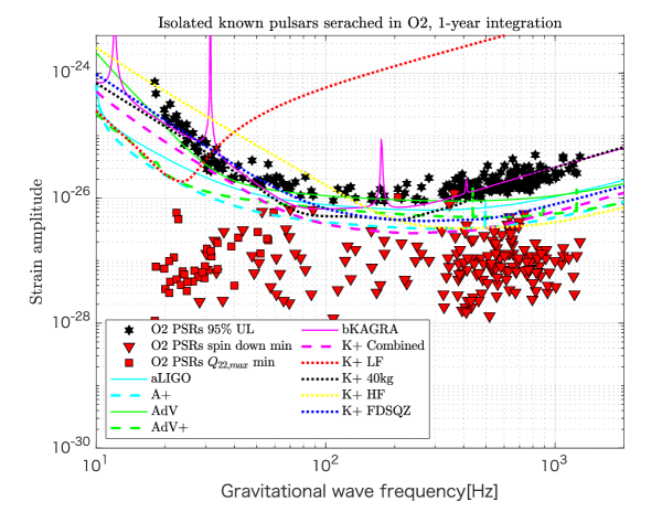
Figure 5 shows the detector sensitivity curves for CW search (assuming 1 year integration, coherent search) as well as the figures of merit for the pulsars that the LIGO-Virgo collaboration has searched for using O2 data LVC_CW_O2CW_APJ_2019 . It is clear that KAGRA+ HF is more useful for CW search.
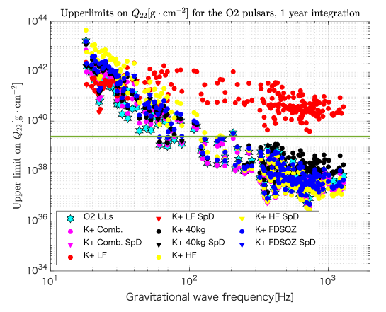
Figure 6 shows the upper limits on that LIGO and Virgo obtained in their O2 search (stars), as well as possible upper limits that are expected by using various configurations of KAGRA+ for the same pulsars. The horizontal thick line indicates the theoretical maximum for for a normal NS. The LIGO-Virgo collaboration has already beaten at higher frequencies than Hz. KAGRA+ LF does not have any power to explore normal NS CWs.
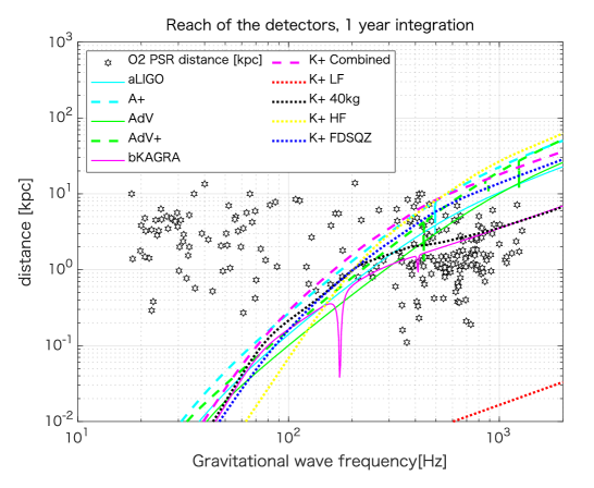
It is possible to conduct unknown pulsar search (e.g., all-sky search, wide-band frequency search). In this case, a possible figure of merit is reach of a detector, which is shown for various detector configurations in Fig. 7, assuming coherent 1 year integration (although it is impossible in practice to conduct a fully coherent unknown pulsar search due to computational resource limitation). This plot again shows that we may be able to have more chance of detection if we put more emphasis on higher frequencies.
We can quantitatively compare performances of various configurations of possible KAGRA upgrades by introducing the gain in the SNR averaged over relevant frequencies. Namely, we define the ratio for the configurations and where is defined in Eq. (5) and a similar equation holds for the configuration. In the case of a continuous wave search, we may be interested in the sensitivity at higher frequency, say, Hz and kHz where the possible constraints on would be the tightest. For “KAGRA+” and “bKAGRA”, ’s then are 1.04 (“40kg”), 3.27 (“FDSQZ”), 5.89 (“HF”), and 4.53 (“Combined”).
6.2 Magnetar flares and pulsar glitches
- Scientific objective
Giant flares in soft gamma-ray repeaters (SGR) which are a class of strongly magnetized NSs, so-called magnetars, were observed: March 5, 1979 (SGR 0526-66); August 27, 1998 (SGR 1900+14); December 27, 2004 (SGR 1806-20). Event rate is quite rare, but huge amount of energy is known to be radiated in EM X and gamma bands. For example, in the last SGR 1806-20 hyperflare, the peak luminosity was erg/s and total energy released in a spike within 1 second was estimated as ergs 2005ApJ…628L..53I . Quasi-periodic oscillations were also observed in the burst tail. Their frequencies are 20-2000 Hz, and are identified by seismic modes excited in magnetar flare. The (quasi)-periodic oscillations are separately discussed in Sec. 6.3. The property and mechanism of the flare are not certain at present, owing to limited number of the events. Especially, the energy carried by GWs is unclear. Theoretical estimate of GW energy associated with flares ranges from erg 2001MNRAS.327..639I ; 2011PhRvD..83j4014C to erg 2011MNRAS.418..659L ; 2012PhRvD..85b4030Z . Dipole field-strength derived by stellar spin and its time-derivative is normally used for the energy deposited before a flare, but much stronger fields might be hidden inside. Thus, the problem will be solved only by actual observations due to many uncertain factors. Actually, GW energy at the SGR 1806-20 hyperflare was limited by LIGO. At that time, one interferometer at Hanford was operated. Upper limit on the GW amplitude is Hz-1/2 and GW energy is less than erg Abbott:2007zzb . It is very important to further proceed the similar argument to each flare observation.
Another interesting astrophysical event is a pulsar glitch.
Sudden change in spin angular frequency is
in a typical giant glitch and
rotation energy changes by
ergs
as for a maximum value.
The change is likely to be much smaller, since the rearrangement of stellar structure
is partial in the transition.
- Observations and measurements
These burst events will be probably first detected in EM signs, and GW signals should be carefully searched at the burst epoch.
There is no reliable waveform, so that GW signals are identified by combinations of multiple detectors.
The burst is a dynamical event in a timescale of millisecond, and
therefore a sharp peak at kHz range is expected.
Coincidence among different GW/EM detectors is crucial.
The observational strategy of GW analysis may depend on the EM information.
When QPO frequencies are identified in EM data, we should search for GW counterparts in the same frequency range.
GW signals in LIGO O2 data2019ApJ…874..16 were searched for magnetar bursts , which are less energetic events. Two software packages, X-Pipeline and STAMP were used: Clusters of bright pixels above a threshold in each time-frequency map are searched in the X-Pipeline, and directional excess power due to arrival time-delay between detectors in the STAMP.
- Future prospects
As for the future extension of bKAGRA, improvements in a higher frequency band are favored for these events. If we fix the frequency of the signal to 1 kHz, SNR ratios of KAGRA+ to bKAGRA at 1 kHz are 40kg 1.03, FDSQZ 3.98, HF 7.47, Combined 5.01. However, it is not clear at present to predict the detection level of meaningful signals by improvements. We will catch them or upper limits by chance, when bursts will happen. The stable operation is desirable.
6.3 Stellar oscillations
- Scientific objective
In order to observationally extract the properties of astronomical objects, asteroseismology is a very powerful technique, where one could get the information about the objects via their specific frequencies. This is similar to seismology in the Earth and helioseismology in the Sun. For this purpose, GWs must be the most suitable astronomical information, owing to their high permeability. In fact, several modes in GWs are expected to be radiated from the compact objects KS99 , and each mode depends on different aspect of internal physics. The GWs have complex frequencies, because the GWs carry out the oscillation energy, where the real and imaginary parts correspond to the oscillation frequency and damping rate, respectively. So, by identifying the observed frequencies (and damping times) of GWs to the corresponding specific modes, one would get the physics behind the phenomena. In general, the GWs are classified into two families with their parity. The axial parity (toroidal) oscillations are incompressible oscillations, which do not involve the density variation, while the polar parity (spheroidal) oscillations involve the density variation and stellar deformation. Thus, from observational point of view, the polar type oscillations are more important, although those are coupled with the axial type oscillations on the non-spherical background.
- Observations and measurements
Some of the GWs from NSs are classified in the same way as the oscillations of usual (Newtonian) stars. That is, the fundamental () and the pressure () modes are excited as acoustic oscillations of NSs, while the gravity () modes are excited by the buoyancy force due to the existence of the density discontinuity or composition gradients inside the star. The Rossby () modes are also excited by the Coriolis force in the rotating stars, although they are axial parity oscillations. In addition to these modes associated with the fluid motions, the oscillations related to the spacetime curvature are also excited, i.e., the so-called GW () modes, which can be discussed only in the relativistic framework. The typical frequencies of , , , and modes for standard NSs are around a few kHz, higher than kHz, smaller than a hundred Hz, and around 10 kHz, respectively KS99 . With these specific modes from the NSs, it has been discussed to extract the NS information via the direct detection of GWs.
One of the good examples of the GW asteroseismology may be the results shown by Andersson and Kokkotas AK96 ; AK98 , where they found the universal relations for the frequencies of the and modes as a function of the average density of star and the compactness, respectively, almost independently of the EOS for NS matter. This is because the frequency of mode, which is an acoustic wave, should depend on the crossing time inside the star with the sound velocity, while the frequency of mode is strongly associated with the strength of the gravitational field. So, if one would simultaneously detect two modes in GWs from the NS, one could get the average density and compactness of the source object, which tells us the NS mass and radius. On the other hand, mode GWs may tell us the existence of the density discontinuity due to the phase transition F87 ; STM01 ; MPBGF03 ; SYMT11 , or they may become more important in the newborn NSs or protoneutron stars (PNSs) RG92 ; FGP07 ; PAH16 . The nonaxisymmetric mode oscillations may also be interesting due to their instability against the gravitational radiations A98 ; FM98 . That is, for highly rotating case, the GW amplitude can exponentially grow up due to the instability, which may become a detectable signal. Eventually, GW amplitude would be suppressed via nonlinear coupling AFMSTW03 . We note that even the mode oscillations may become unstable in rapidly rotating relativistic NSs GGKZ11 . In any case, the detection of GWs from the isolated (cold) NS may be quite difficult with the current GW detectors, because most of their frequencies are more than around kHz.
On the other hand, the detection of GWs from the PNSs would be more likely if they are formed within our galaxy. This is because, since the PNSs are initially less massive and larger radius, i.e., their average density is smaller than the cold NSs, one can expect the frequency of mode GW would be smaller than the typical one for cold NSs. In practice, the mode frequency of PNS is around a few hundred Hz in the early phase after core-bounce ST16 . However, the studies of the asteroseismology in PNSs are very few, unlike cold NSs. This is because of the difficulty for providing the background models. That is, the cold NSs can be constructed with the zero-temperature EOS, i.e., the relation between the energy density and pressure, while one has to consider the distribution of the electron fraction and entropy per baryon together with the pressure distribution as a function of density to construct the PNS models. But, such distributions can be determined only after the numerical simulation of core-collapse supernovae. Even so, the study of asteroseismology in PNSs is becoming possible with the numerical data of simulation.
Up to now, two different approaches are proposed for providing the PNS models, i.e, one is that the PNS surface is defined with a specific density around g/cm3 ST16 ; SKTK17 ; MRBV18 ; SKTK19 ; Sotani19 , and the other is that the oscillations inside the shock radius are considered TCPF18 ; TCPOF19 , where the different boundary conditions should be adopted according to the approaches. In contrast to the cold NSs, matter widely exists outside the PNSs, which makes difficult to treat the boundary of the background models. Anyway, even with either approach, it seems that the mode frequencies of GWs are expected to range in wide frequencies and that such frequencies would change with time. If one could identify the frequencies of GWs with a specific mode, it must be very helpful for understanding the physics of PNS cooling via understanding of the PNS properties. In practice, the time evolution of the identified frequencies is considered as a result of the changing of the PNS mass and radius, i.e., the mass increases due to the accretion and the radius decreases due to the both of a relativistic effect and neutrino cooling, with time. So, in the same way as for the cold NSs, if one could simultaneously identify the frequencies with the and modes GWs from PNSs, one would get the information of the average density and compactness at each time, which enables us to know the evolution of mass and radius of PNSs SKTK17 . That is, unlike the cold NSs, in principle one can expect to make a severe constraint on the EOS even with one event of GW detection. It should be emphasized that the frequencies of mode GWs from the PNSs becomes typically around a few kHz, because the compactness is smaller than that of cold NSs.
- Future prospects
We make a comment about the detectability of these modes in GWs. The GW amplitudes have been discussed in Ref. AK96 ; AK98 for isolated cold NSs, assuming the radiation energy of GWs with each mode. Since the radiation energy with each mode can not be estimated as far as one examines the GW asteroseismology with linear perturbation analysis, one should eventually estimate such radiation energy with numerical simulation to see the detectability. The situation in PNSs born after the core-collapse supernova is the same. Even so, adopting the formula shown in Ref. AK96 ; AK98 , the effective gravitational amplitude of mode from the PNSs may be estimated with its energy, , at each time step as
| (10) |
where and denote the frequency of considering mode and the distance to the source object, respectively SKTK17 . The total radiation energy of the mode in the GWs from PNS, , may be estimated as , where denotes the damping time of mode with the frequency of at each time step. In this estimation, we assume that mode GW emission would last for the duration of , as the frequency of evolves, where we simply adopt ms. Then, the effective amplitude is plotted as in Fig. 8, where the circles, squares, diamond, triangles, and upside-down triangles correspond to the expectations with , , , , and , respectively.
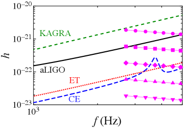
To detect the GW signal due to the NS oscillations, improvements in a higher frequency must be more suitable, although the amount energy of GWs are unknown at present. If we fix the frequency of the signal to 1 kHz as in the previous section 6.2, the SNR ratios of KAGRA+ to bKAGRA at 1 kHz are 40kg 1.03, FDSQZ 3.98, HF 7.47, Combined 5.01. The improvements even in a middle frequency band may be suitable for detecting the -mode GWs from the PNS, but it must be acceptable only in the early phase after the core-bounce, because the frequency increases with time and eventually becomes kHz.
7 Supernovae
7.1 The explosion mechanisms and the GW signatures
- Scientific objective
Accumulating observational evidence from multi-wavelength EM observations such as of ejecta morphologies and spatial distributions of heavy elements have all pointed toward CCSNe being generally aspherical (e.g., casA ; tanaka17 and references therein). However, these signals are secondary for probing the multidimensionality of the supernova engine because they are only able to provide images of optically thin regions far away from the central core. The GWs from CCSNe are the primary observables, which imprint a live information of the central engine.
From a theoretical point of view, understanding the origin of the explosion
multidimensionality is indispensable for
clarifying the yet uncertain CCSN mechanisms.
After a half-century of continuing efforts,
theory and neutrino radiation-hydrodynamics simulations
are now converging to a point that multi-dimensional (multi-D)
hydrodynamics instabilities play a pivotal role in the
neutrino mechanism (bethe ), the most favoured scenario
to trigger explosions.
In fact, self-consistent
simulations in three spatial dimensions (3D)
now report shock revival of the stalled bounce shock into explosion
by the multi-D neutrino mechanism
(see bernhard16 ; janka16 ; burrows13 ; Kotake12 for recent reviews).
- Observations and measurements
The most distinct GW emission process commonly seen in recent self-consistent three-dimensional (3D) models is associated with the excitation of core/PNS oscillatory modes (e.g., radice18 ; andresen18 ; andresen17 ; kuroda16 ). The dominant modes are the quadrupolar () deformations of the PNS excited by the non-spherical mass accretion onto it (see also Sec. 6.3). The characteristic GW frequency increases almost monotonically with time due to an accumulating accretion onto the PNS, which ranges from to 1000Hz (see astone18 for the dedicated scheme to detect the ramp-up GW signature from the noises).
In addition to the prime GW signature, the Standing Accretion Shock Instability (SASI) (e.g., thierry15 ) has been also considered as a key to generate GW emission in the postbounce supernova core. It has become apparent radice18 ; andresen18 ; kuroda16 that the predominant GW emission from CCSNe is produced in the same region behind the postshock region where both the SASI and neutrino-driven convection vigorously develop (e.g., Kotake13 for a review). The GW emission from this region–from just above the neutrinospheres at densities of roughly 1011 g/cm3 and inward–is determined by the effects of the super-nuclear EOS, as well as the impact of hydrodynamic instabilities present in the post-shock flow (e.g., andresen17 ). The typical frequency of the SASI-induced GWs is in the range of 100 – 250 Hz, which is in the best sensitivity range of the currently running interferometers.
Rapid rotation in the iron core leads to significant rotational flattening of the collapsing and bouncing core, which produces a time-dependent quadrupole (or higher) GW emission (e.g., ott_rev for a review). For the bounce signals having a strong and characteristic signature, the iron core must rotate rapidly enough333Although rapid rotation and the strong magnetic fields in the core is attracting great attention as the key to solve the dynamics of collapsars and magnetars, one should keep in mind that recent stellar evolution calculations predict that such an extreme condition can be realized only in a special case woos06 ( 1% of massive star population).. The GW frequency associated with the rapidly rotating collapse and bounce is in the range of Hz.
Another distinguished feature of GWs from a CCSN is a circular polarization. The importance of detecting circular GW polarization from CCSNe was first discussed
by Hayama16 in the context of rapidly rotating core-collapse.
More recently Hayama18 presented analysis of the GW
polarization using results from 3D general-relativistic simulations of a non-rotating
star kuroda16 .
The amplitude of the GW polarization was shown to become larger for
the 3D general-relativistic model that exhibits strong SASI activity.
The non-axsymmetric flows associated with spiral SASI give rise to the circular polarization.
If detected, it will provide us a new probe into the SASI activity in the preexplosion supernova core.
Note that the spiral SASI develops mainly outside of the PNS, so that the circular polarization from the
spiral SASI has different features in the spectrogram comparing to the stochastic, weak circular polarization
from the PNS oscillations that have no preferential direction to develop Hayama18 .
By estimating the SNR of the GW polarization,
they pointed out the possibility that the
detection horizon of the circular polarization could extend by more than a
factor of several times farther comparing to that of the GW amplitude.
In order to detect the GW circular polarization with a high SNR, the joint GW observation
with KAGRA in addition to two LIGOs and Virgo is indispensable.
- Future prospects
Each phase of a CCSN has a range of characteristic GW signatures and the GW polarization that can provide diagnostic constraints on the evolution and physical parameters of a CCSN and on the explosion hydrodynamics. The GW signatures described in this section commonly appear in the frequency range of - Hz in recent simulations of the CCSN. Among them, the PNS oscillatory modes are currently recognized as the model-independent GW signature. The characteristic frequencies of the fundamental () modes are predominantly dependent on the PNS mass () and the radius (), however, in a non-trivial manner sotani17 . In order to break the degeneracy, the detection of other eigen-modes ( modes) of the PNS oscillations is mandatory. In fact, the GW asteroseismology of the PNS has just started forne19 ; morozova18 ; sotani17 (see also Sec. 6.3). The outcomes of which should reveal the requirement of KAGRA (and the next-generation detectors) to detect the whole of the eigenmodes (presumably extending up to several kHz) for the future CCSN event. This could be done in the next five years.
For the detectability of GWs from PNSs, see Sec. 6.3. The GWs due to SASI for a Galactic event may be detected with the SNR of the GW signals predicted
in the most recent 3D CCSN models in the range of 4 – 10 for the aLIGO andresen17 . With the third-generation detectors online (e.g., Cosmic Explorer), these signals would be never missed for the CCSN events throughout the Milky way. A current estimate of SNR for the GWs from rapidly rotating collapse and bounce based on predictions from a set of 3D models using a coherent network analysis
shows that these GW signals could be detectable up to
about kpc for the most rapidly rotating model (hayama15 , see also powell19 ; gossan16 ).
If the spectra of the supernovae are assumed to be flat in the frequency range of 100 Hz - 1 kHz, we can quantitatively compare performances of various configurations of possible KAGRA upgrades by defining the SNR ratio for the configurations
and where is defined in Eq. (5) and a similar equation holds for the configuration. For the frequency range between Hz and kHz, the SNR ratios of KAGRA+ to bKAGRA averaged over relevant frequencies are 40kg 1.51, FDSQZ 2.35, HF 3.43, Combined 3.55. However, since the spectral evolution of the CCSN GWs has not been completely clarified yet and it does depend upon the details of CCSN modeling (such as on the initial rotation rates and the progenitor masses), it is too early to make a quantitative discussion about the best-suited sensitivity curves for KAGRA+. Because recent CCSN simulations indicate that the important GW frequency to unveil the physics of CCSNe will be Hz, all the candidate upgrades except for LF should help enhance the chance of detection.
8 The early Universe
8.1 GWs from inflation
- Scientific objective
Inflation, an accelerated expansion phase of the very early Universe,
was proposed in the 1980s to solve problems in the standard model of
the Big Bang theory, such as the horizon, flatness, and monopole
problems inflation1 ; inflation2 ; inflation3 ; inflation4 . A key
feature of inflation is that the rapid expansion stretches quantum
fluctuations in a scalar field to classical scales and generates
primordial density fluctuations
scalar1 ; scalar2 ; scalar3 ; scalar4 ; scalar5 , which become the seeds
of galaxies. The nearly scale invariant spectrum of scalar
perturbations, predicted by the inflationary theory, is strongly
supported by cosmological observations of the cosmic microwave
background and galaxy surveys. The same mechanism also applies to
quantum fluctuations in space-time, which produce a stochastic
background of GWs over a wide range of frequencies
with a scale-invariant power spectrum tensor1 ; tensor2 ; tensor3 . The detection of inflationary GWs is a key to test
inflation and distinguish a number of models since the amplitude and
spectral index strongly depend on the model.
- Observations and measurements
The amplitude of the GWs is typically far below the sensitivity of the ground-based detectors. The dimensionless parameter, , which describes the energy density of GWs per logarithmic frequency interval, is roughly given by for a scale invariant primordial spectrum , where is the Hubble expansion rate during inflation. Inflation predicts a slightly red-tilted spectrum, which further reduces the amplitude at high frequency. For example, the model predicts at Hz for chaotic inflation and for inflation, while the cross correlation between LIGO, Virgo, and KAGRA with their final design sensitivities is expected to reach a stochastic background of . For details on the shape of the spectrum, see Kuroyanagi:2008ye ; Kuroyanagi:2014qaa .
Note that a search for a stochastic GW background is performed by cross-correlating data from different detectors over a long time period. The sensitivity is determined by noise curves of the multiple detectors as well as the observation time. Since the two detectors of LIGO have advantages in both sensitivity and observation time, the sensitivity of the four-detector network will be dominated by LIGO detectors, while KAGRA with the current design sensitivity would not contribute to increase the overall sensitivity. Currently LIGO-Virgo O2 data provide an upper limit of for a scale invariant spectrum LIGOScientific:2019vic .
Although the ground-based detectors are not sensitive enough to detect standard inflationary GWs, some models going beyond the standard picture predict a blue-tilted spectrum, e.g, string gas cosmology Brandenberger:2006xi , super-inflation models Piao:2004tq ; Baldi:2005gk , G-inflation Kobayashi:2010cm , non-commutative inflation Calcagni:2004as ; Calcagni:2013lya , particle production during inflation Cook:2011hg ; Mukohyama:2014gba , Hawking radiation during inflation Mohanty:2014kwa , a spectator scalar field with small sound speed Biagetti:2013kwa , massive gravity Fujita:2018ehq , and so on. The amplitude of the inflationary GW spectrum is constrained at low frequencies by the cosmic microwave background , but the amplitude can be large at the frequency of Hz if the spectrum is blue-tilted. There would be a chance for the ground-based detectors to detect inflationary GWs if the spectral index of the spectrum is larger than .
Another possibility for the ground-based detectors is to probe a non-standard Hubble
expansion history of the early Universe
Peebles:1998qn ; Giovannini:1998bp ; Giovannini:1999bh ; Giovannini:1999qj ; Tashiro:2003qp ; Giovannini:2008tm .
The information on the expansion rate, which is determined by the
dominant component of the Universe, is imprinted in the spectrum of
inflationary GWs. For a scale invariant primordial
spectrum, the spectral dependence of the stochastic background becomes
, where is the EOS of the Universe. In the standard cosmological model, the
matter-dominated () and radiation-dominated () phases
yield and , respectively. When
one considers a kination dominated phase () soon after inflation,
the spectral amplitude is enhanced at high frequency by the dependence
and peaks at the frequency corresponding to
the size of the Universe at the end of inflation, which is typically
higher than Hz. Although it is difficult to find a
case where GWs are detectable by the ground-based
experiments satisfying the Big-Bang nucleosynthesis (BBN) bound Figueroa:2018twl ; Ahmad:2019jbm , for Hz, the upper bound on the stochastic
background is still helpful to explore early-Universe physics beyond
the standard cosmology.
- Future prospects
The SNR for a stochastic GW background is computed by taking cross-correlation between detector signals Allen:1997ad , and given by
| (11) |
where is the Hubble constant, is the observation time, and is the noise spectral density with and labeling two different detectors. The overlap reduction function is given by the detector responses of the two polarization modes and as
| (12) |
where describes the position of the detector and specifies the propagation direction of GWs. For a network of detectors, the total SNR is given by
| (13) |
As seen in the overlap reduction function, the SNR depends on the distance and relative orientation of the detectors. For KAGRA, correlating with AdV+ is better than with A+ because of the relative orientation. Assuming the flat spectrum of , the sensitivities of the pair of KAGRA and AdV+ to with are for bKAGRA, for LF, for 40kg, for FDSQZ, for HF, and for Combined. The lower frequency upgrades give better sensitivities. However, the sensitivity between two A+ is , which is an order of magnitude better than those with KAGRA because of much closer separation of the detector pair. Therefore, KAGRA is not good for detection but will be able to play an important role for determining the spectral shape and measurig anisotropy, non-Gaussianity and polarizations, which are discussed in Sec. 8.3.
8.2 GWs from phase transition
- Scientific objective
The thermal history of the Universe after BBN,
which takes place at a temperature scale of order of 1 MeV,
has been well established thanks to amazing progress made by cosmological
observations.
On the other hand, our knowledge about the Universe earlier than BBN is
quite limited.
If we extrapolate our understanding of particle physics,
several phase transitions should occur
in such early stages of the Universe.
These include the QCD phase transition,
the electroweak phase transition, the GUT phase transition and
some phase transitions of new models beyond the Standard Model of particle
physics.
The nature of a phase transition is classified according to
the evolution of the order parameter: first-order or second-order.
In addition, the case where the order parameter changes smoothly
and no phase transition occurs is referred to as a crossover.
For a first-order phase transition, a latent heat is released,
supercooling emerges and phases are mixed like boiling water.
Non-uniform motion of vacuum bubbles during the first-order phase transition,
GWs are produced.
Therefore, one can survey new physics models
involving a first-order phase
transition by observing GWs Grojean:2006bp .
- Observations and measurements
GWs produced by the first-order phase transition in the early Universe are stochastic: isotropic, stationary and unpolarized. They are characterized only by the frequency. There are three known sources for GWs from the first-order phase transition: collisions of vacuum bubble walls, sound waves in the plasma and plasma turbulence. In general, one has to sum these contributions. For typical non-runaway bubbles, the contribution from sound waves is dominant and the peak energy density 444The energy density of gravitational waves and the power spectral density is related through . is roughly Caprini:2015zlo
| (14) |
and the peak frequency is
| (15) |
Here, is the transition temperature,
is the ratio of the released energy (latent heat)
to the radiation energy density, is the inverse of the time duration
of the phase transition, is the Hubble expansion parameter at ,
is the ratio of vacuum energy converted into fluid motion, and
is the bubble wall velocity.
If one selects a new physics model and chooses a model parameter set,
one can compute the finite temperature effective potential, from which
the above quantities are derived.
Namely, the above quantities are functions of the underlying model parameters.
Therefore, the number of free model parameters can be generally reduced by measuring the stochastic GW spectrum.
- Future prospects
Among new physics models that involve phase transitions, models with an extended Higgs sector achieving the electroweak phase transition are of most importance and should be addressed. Although the Higgs boson has been discovered at the CERN Large Hadron Collider and the spontaneous breaking of the electroweak symmetry has been established, the dynamics of the electroweak symmetry is still unknown. The baryon asymmetry of the Universe may be accounted for by electroweak baryogenesis, which requires a strongly first-order electroweak phase transition. Since the transition temperature of the electroweak phase transition is of the order of 100 GeV, unfortunately the peak frequency of the predicted GWs spectrum falls in the range of Hz to 0.1 Hz, regardless of the details of the extended Higgs models. Therefore, the detection of GWs from the electroweak phase transition and determination of the model parameters of extended Higgs models are challenging for KAGRA upgrade and need future space-based interferometers, such as LISA and DECIGO Kakizaki:2015wua ; Hashino:2018wee . Conversely, one can envisage and construct hypothetical models with the phase transition temperature of GeV to GeV so that the peak frequency matches with the KAGRA frequency band Dev:2016feu . Even in such models, an enormously large latent heat and/or an very long transition duration are necessary for GW signals to hit the sensitivity curves for KAGRA upgrade candidates. Another issue concerns uncertainties in computing the spectrum of generated stochastic GWs at a first-order phase transition. In particular, numerical simulations of the dynamics of nucleated bubbles are rather cumbersome. With the development of computational techniques, the result in Eq. (14) might be revised by one order of magnitude or more. Therefore, although it is difficult to predict the detectability of GWs from a phase transition, KAGRA will play an important role in constraining models of first-order phase transitions that take place at temperatures of around GeV to GeV.
8.3 Distinguishing the origins of the GW backgrounds
- Scientific objective
GWs generated in the early Universe are typically in
the form of a stochastic background, which is a continuous noise-like
signal spreading in all directions, while numerous astrophysical
GWs also become a stochastic background by overlapping
one another. Even if a stochastic background is detected, it may be
difficult to identify its origin among many cosmological and
astrophysical candidates.
- Observations and measurements
A standard data analysis provides information only on the amplitude and the tilt of the spectrum. In order to discriminate the origin of the GW background, we need to go beyond conventional data analysis and extract more information, such as the spectral shape Kuroyanagi:2018csn , anisotropy Allen:1996gp ; TheLIGOScientific:2016xzw , polarization Nishizawa:2009bf ; Abbott:2018utx , and non-Gaussianity (or so-called popcorn background) Drasco:2002yd ; Thrane:2013kb ; Martellini:2014xia . Anisotropy and non-Gaussianity could arise in a GW background formed by overlapping GW bursts. Typical examples are the ones originating from astrophysical sources and cosmic strings. Additional GW polarizations appear when the generation process is related to physics beyond general relativity (see Sec. 9.4). Therefore, they can be used as indicators of specific generation mechanisms.
The spectral shape of the stochastic background depends strongly on its origin and it can be generally used to distinguish a wide range of generation models.
Many models predict a spectral shape spanning a broad range of frequencies. In this case, the ground-based detectors observe a part of the spectrum because of the limited sensitivity range of frequency, and multi-band observations are needed to determine the whole spectral shape. However, some models predict a peaky spectral shape; one good example testable by the ground-based detector network itself is a GW background generated by superradiant instabilities Brito:2017wnc .
One way to obtain the spectral shape in data analysis is to use broken
power-law templates instead of the currently used single power-law
templates Kuroyanagi:2018csn ; Bose:2005fm . The uncertainties in
the parameter determination decrease in proportional to the inverse of
the SNR, and at least SNR is
necessary to obtain useful information on the entire spectral shape.
If detection were made with higher SNR, the analysis could be extended
to the whole spectral shape reconstruction with multiple frequency
bins, which evaluates the spectral index in each bin (see
Figueroa:2018xtu for the discussion for LISA, which could be
applied to ground-based experiments).
- Future prospects
In general, a higher SNR is necessary not only to determine the spectral shape but also to obtain the above mentioned additional properties of the stochastic background. Since inflationary GWs have a red-tilted spectrum in terms of strain amplitude, an improvement of sensitivity at lower frequency would be helpful to test more properties of the stochastic background. On the other hand, as previously mentioned, the sensitivity of the ground-based detectors is not enough to detect a standard inflationary GW background, and a blue-tilted spectrum is necessary to enhance the amplitude for detection. If , where we define the spectral tilt as , an improvement of sensitivity at higher frequencies becomes important (see Fig. 1 of Kuroyanagi:2018csn ). Astrophysical GWs also have a blue-tilted spectrum , but when the tilt is not so steep, sensitivity at mid-frequencies (Hz) is more important.
Apart from sensitivity for the amplitude, multiple detectors facing different directions provide independent information about anisotropy and polarization, and thus the inclusion of KAGRA is essential.
9 Test of gravity
9.1 Test of consistency with general relativity
- Scientific objective
There are currently no alternatives to Einstein’s GR that are physically viable.
As such, one cannot test GR by comparing the data with waveforms in alternative theories.
Instead, one can test for the consistency of the signal with GR.
In doing so, one must ensure that any deviation from GR cannot be attributed to noise artifacts, but instead are intrinsic to the GW signal itself.
However, this must be done without explicitly assuming an alternative model for gravity that governs the morphology of the GW signal.
- Observations and measurements
Existing efforts largely focus on comparing different portions or aspects of the signal and require consistency amongst them.
For example, one can verify the self-consistency of the post-Newtonian description of the inspiral phase, and from the phenomenological GR model of the merger-ringdown LiEtAl:2012a ; LiEtAl:2012b ; Agathos:2013upa ; Cornish:2011ys ; Sampson:2013jpa ; Meidam:2017dgf .
In addition, one can also test the final remnant mass and spin, as determined from the low-frequency (inspiral) and high-frequency (post-inspiral) phases of the signal for mutually consistent Ghosh:2016qgn ; Ghosh:2017gfp .
Furthermore, one can also compare the residual signal after subtracting the best-fitting GR waveform to the expected statistical properties of the noise.
For the first set of BBH detections, all tests so far have not revealed any significant deviations from GR TheLIGOScientific:2016src ; TheLIGOScientific:2016pea ; Abbott:2018lct ; LIGOScientific:2019fpa .
Instead, constraints on various possible beyond-GR effects have been placed.
For example, the fractional deviations to the lowest post-Newtonian parameters have been constrained to tens of percent, whereas the higher post-Newtonian orders and the merger-ringdown parameters are constrained to around a hundred percent.
Moreover, the possibility of dipolar radiation has been constrained to the percent level, and the mass of the graviton has been constrained to .
- Future prospects
In the future, as the LVK network operates at their full strengths, we can anticipate several effects that will improve our ability to constrain general relativity. Firstly, the improved detection rate will allow us see many events for which the different aspects of their dynamics are covered by the network’s sensitive frequencies. Secondly, more detections also means that our constraints will be improved statistically. While we do not expect improvements of orders of magnitude, it will help to shrink the parameter space of possible deviations from GR. Thirdly, a full LVK network will greatly enhance tests that require multiple detectors, including tests for alternative polarisations (see Sec. 9.4). These tests are expected to greatly improve as KAGRA, as the fourth detector, improves its sensitivity. Finally, the prospect of observing novel source classes, including highly eccentric systems, highly precessing systems and even head-on collisions will open up a entirely new suite of tests.
In the era of KAGRA+, we expect more detections of BBH and BNS, and anticipate detections of BH-NS systems. The precise way in which KAGRA+’s sensitivity develops will govern the way it will contribute to tests of GR. For example, with the focus on low-frequency sensitivity, one improves the insight into the merger and ringdown of heavy BHs, where the gravitational fields are the strongest. In contrast, high frequency sensitivity allows one to track lower mass binary merger for a longer period of time, which improves the precision of the consistency checks. Additionally, by improving the sky coverage and increasing the multiple-detector live time, KAGRA+ will increase the number of detected events and thereby reducing the statistical errors due to detector noise by combining results from multiple events.
9.2 GW generation in modified gravity
- Scientific objective
We can raise several motivations to study modified gravity: a) GR is not ultraviolet (UV) complete theory. It should be modified to describe physics near Planck scale. b) Cosmology based on GR requires dark components to explain the observed Universe, such as dark matter and dark energy. It is attractive if we can naturally explain the observed Universe by a well-motivated modification of gravity without introducing cosmological constant. c) To test GR, it is not enough to know the prediction based on GR when we use GWs as a probe. Since GW data is noisy, an appropriate projection of the data in the direction predicted by the possible modification of gravity is necessary to obtain a meaningful constraint.
As possible modifications of gravity, there are several categories. One is to add a new degree of freedom like a scalar field in scalar-tensor gravity. Such a kind of extra degrees of freedom is strongly constrained by existing observations, since they introduce a fifth force. There are various ways, however, to hide the fifth force. 1) Sufficiently small coupling to the ordinary matter. 1-a) Coupling through higher derivative terms, which becomes important only under strong field environment. 1-b) Some non-linear mechanism to reduce the coupling like Chameleon/Vainstein mechanism Khoury:2003aq ; Vainshtein:1972sx . 2) Giving a sufficiently large mass to the field that mediates the fifth force.
There is also a possibility to modify gravity without introducing a new degree of freedom.
One example is so-called minimal extension of massive gravity. Phenomenologically,
we can give small mass to graviton in this kind of model, but the graviton mass at the
present epoch is already strongly constrained by the observation of GW170817.
- Observations and measurements
We focus on compact binary inspirals. In this context, the most probable modification of the generation mechanism of GWs is the one caused by the change in orbital evolution. The orbital evolution is governed by two aspects. One is the conservative part of the gravitational interaction and the other is the dissipative effects of radiation. It is not so obvious which effect is more important even in the weak field regime. Hence, we need a little more careful investigation of each model.
Whichever effect dominates, the main purpose of this study is the same. What we want to clarify is whether or not there exists a new effective propagating degree of freedom which appears only when we consider extremely compact objects like BHs and NSs.
There might be various possibilities. From the observational point of view it is convenient to introduce the parametrized post-Einstein (PPE) framework YunesPretorius2009 . The waveform of quasi circular inspiral in Fourier domain will be given in the form of
| (16) |
in GR. The waveform is characterized by the functions and and they are modified in the extended theories like
| (17) |
with . Since the test of gravity using GW data is more sensitive to the modification in the phase , we will focus on it.
The smallest non-vanishing value of is related to the leading post-Newtonian order. The -th post Newtonian correction appears as . Here we list representative possible modifications of gravity with the post-Newtonian order of the leading correction in phase in Table 8. BH evaporation is negligible in the ordinary scenario, but can be accelerated if there are many massless hidden degrees of freedom. For the dipole radiation to be emitted, charge not proportional to the mass of each constituent object is required. One typical example is the scalar tensor theory. Although BHs are thought not to bear a scalar hair in many cases, they can have a scalar charge in some models like in Einstein-Gauss-Bonnet-dilaton theory Yagi:2011xp . If we naively consider that gravitons have non-vanishing mass, the dispersion relation is also modified to give 1PN order correction, although this is not the effect in the generation of gravitational waves. However, if we consider covariant theories of massive gravity, we need to consider a bigravity model Hassan:2011zd . As a modification that appears at the 1PN order, one may think of a model in which the mass of each constituent object depends on the Newton potential.
| modification | post-Newtonian order | References |
|---|---|---|
| variable Newton’s constant | -4PN | Yunes:2009bv |
| BH evaporation | -4PN | Yagi:2011yu |
| dipole radiation | -1PN | Will:1989sk |
| non-covariant massive graviton | 1PN | Will:1997bb |
| dynamical Chern-Simons gravity | 2PN | Yagi:2012vf |
As a typical modification of GR, the scalar-tensor theory is often discussed. If the binary members have some scalar charges coupled to the extra degree of freedom, we have dipolar radiation. Although the overall magnitude also depends on the coupling strength, if we focus only on the frequency dependence, the flux due to dipolar radiation is larger at a low frequency by the factor compared with that due to GW radiation. On the other hand, the extra scalar degree of freedom changes the conservative part of the force, but there is no such enhancement in the sense of post Newtonian order. Hence, at low frequency, where the modification to the conservative gravitational interaction can be neglected.
For the modification that predicts negative post-Newtonian order, the deviation form GR is relatively larger at lower frequencies, compared with GR contributions. Therefore, it is not so easy for GW observations to compete with the constraint from the observations at lower frequencies, such as the pulsar timing.
There are some more detailed aspects that cannot be expressed by the PPE framework. One possibility is the spontaneous scalarization. When we consider BNS, each NS in isolation may not have a scalar charge. However, there is a region in the model parameter space in which instability occurs as the binary separation decreases and both NSs get charged. Another possibility is that the mediating scalar field is massive. This is quite likely to avoid the instability similar to the spontaneous scalarization to occur in the whole Universe after the temperature of the Universe becomes or lower. If the instability occurs, the success of the big-bang nucleosynthesis will be significantly damaged. This gives the constraint on the mass of the mediating field to be greater than eV or so Ramazanoglu2016 , which is comparable to the constraint from pulsar timing (PSRJ0348+0432). On the other hand, ground-based detectors are sensitive to modification if the mass is smaller than eV. If the mass is in the range between these two, the existence of the extra degree of freedom might be probed only by GWs.
Basically we check the deviation of the observed GW signal from GR templates.
For this purpose, it is better to have a better theoretical template based on each candidate of
modified gravity. In particular this demand is higher when we consider the models
whose leading order modification appears at the positive post-Newtonian order.
In such models, we have more chances to observe the largest deviation at
the final stage of inspirals. In many cases, this task remains to be a challenge for the theorists.
- Future prospects
As long as we consider BHs with the mass larger than a few times the solar mass and NSs, it seems difficult to use a high frequency band to give constraints on modified gravity. In the case of BHs, we do not have much signals at very high frequencies. In the case of binary NSs, high frequency signal can be expected but it might be difficult to disentangle the effects of modified gravity from the uncertainty of the complex physics of NSs.
In general, when we wish to give a tighter constraint on the parameters contained in the waveform template, broader observational sensitivity band is advantageous. A broadband observation is not necessarily realized by a single detector. It would work well if a wider range of the frequency band is covered by plural detectors as a whole. In this sense, it would be necessary to negotiate among the various plans of future upgrade of detectors.
In near future we will establish a network composed of LIGO, Virgo and KAGRA. On the point of view of detecting modification in the gravitational wave generation, the improvement of the constraints depends on the increase of statistics and finding of some golden events with appropriate binary parameters and a large signal-to-noise.
9.3 GW propagation test
- Scientific objective
The properties of GW propagation are changed when a gravity theory is modified from GR. Particularly, such modifications are paid much attentions at cosmological distance because the extended theories of gravity may explain the accelerating expansion of the Universe. In other words, testing GW propagation can constrain the possible modification of gravity at cosmological distance and give us an implication about the physical mechanism of the cosmic accelerating expansion Lombriser:2015sxa . According to Saltas:2014dha , the modifications of GW propagation in the effective field theory is expressed in general as
| (18) |
and are characterized by four properties: propagation speed , amplitude damping rate , graviton mass , and a source term . Each modification appears differently in a specific theory, but this framework allows us to test many classes of gravity theories at the same time. Among the modifications, the propagation speed is important to test the violation of the Lorentz symmetry and the quantum nature of spacetime (modified dispersion relation). The amplitude damping rate is equivalent to the variation of the gravitational constant for GWs and enables us to test the equivalence principle. The graviton mass is a characteristic quantity in massive gravity. If parity in gravity is violated, it modifies in general the propagation speeds and the amplitude damping rates in Eq. (18) differently for left-handed and right-handed polarizations with opposite signs as shown in Nishizawa:2018srh ; Zhao:2019xmm .
- Observations and measurements
The coincidence detection of GW170817/GRB170817A GW170817PRL brought us the first opportunity to measure the speed of a GW from the arrival time difference between a GW and an EM radiation555Before GW170817/GRB170817A, the measurements of the speed of a GW have done with GWs from BBH based on the arrival time difference between detectors Blas:2016qmn ; Cornish:2017jml ., as was predicted in Nishizawa2014PRD , and constrained the deviation from the speed of light at the level of GW170817:GRB . Based in this constraint on GW speed, a large class of theories as alternatives to dark energy have already been almost ruled out Baker:2017hug ; Creminelli:2017sry ; Sakstein:2017xjx ; Ezquiaga:2017ekz . The graviton mass has been tightly constrained from the observation of BBH mergers in the range of LIGOScientific:2019fpa , which is tighter than that obtained in the Solar system Bernus:2019rgl . On the other hand, the amplitude damping rate has also been measured from GW170817/GRB170817A for the first time in Arai:2017hxj , but the constraint is still too weak, . However, the anomalous amplitude damping rate is one of the prominent signatures of modified gravity, which is likely to be accompanied by the gravity modification explaining the cosmic acceleration, and plays a crucial role when we test gravity at cosmological distance Nishizawa:2019rra .
In generic parity-violating gravity including recently proposed ghost-free theories with parity violation Crisostomi:2017ugk , not only the amplitude damping rate but also the propagation speed are modified, in contrast to Chern-Simons modified gravity in which the GW speed is the speed of light. From GW170817/GRB170817A, since a GW is required to propagate almost at the speed of light, the parity violation in the GW sector of the theory has been constrained almost to that in Chern-Simons gravity, allowing only the amplitude damping rate to differ from GR Nishizawa:2018srh .
- Future prospects
To forecast the abilities to measure the modified gravity parameters with a future detector network including bKAGRA and KAGRA+, we estimate the measurement errors of the model parameters in the modified GW waveform with the Fisher information matrix (For the detail of the analysis, see Nishizawa:2017nef ). For the waveform, we consider the simplest one in which the amplitude damping rate and the graviton mass are assumed to be constant, taking and . Setting is motivated by the existing constraint from GW170817/GRB170817A and is true in most gravity theories including the Horndeski theory Saltas:2014dha . Under the assumptions above, the GW waveform is Nishizawa:2017nef
| (19) |
where is the wave number. The waveform is the one in GR. Then the luminosity distance observed by a GW is interpreted as an effective one, , which differs from the standard one for EM waves, . To break a parameter degeneracy and determine separately, one needs to know a source redshift independently of a GW observation. We assume that the source redshift is obtained somehow from EM observations and impose a prior on with a standard deviation . We will generate 500 binary sources with random sky locations and other angular parameters, having the network SNR , for each case with fixed masses and redshift.
In Table 9, the parameter estimation errors of and with detector networks including KAGRA are shown. The sensitivities are better for heavier binaries and best for BBH. The upper limits on graviton mass are similar to the current constraint and are not expected to be improved significantly with the ground-based detectors in the future. Since the graviton mass affects GW phase more at lower frequencies, the constraints from the planned spaced-based detectors such as LISA Audley:2017drz and DECIGO Sato:2017dkf will be much stronger down to – Yagi:2009zm ; Yagi:2009zz . On the other hand, there are modest improvements of the sensitivity to with the addition of bKAGRA or KAGRA+ to the global detector network. For a measurement of with BBH, the improvement factors of the errors are LF 0.87, 40kg 1.16, FDSQZ 0.99, HF 0.98, Combined 1.35, reaching in the best case.
| source | quantile | bKAGRA | LF | HF | 40kg | FDSQZ | Combined |
|---|---|---|---|---|---|---|---|
| SNR | BBH | 77.4 | 73.9 | 76.6 | 78.0 | 79.6 | 84.8 |
| BBH | 32.3 | 32.9 | 34.2 | 33.9 | 32.3 | 36.6 | |
| BH-NS | 25.1 | 23.7 | 24.8 | 25.2 | 26.4 | 27.2 | |
| BNS | 24.3 | 24.2 | 24.7 | 24.7 | 24.9 | 27.5 | |
| BBH | 1.47 | 1.69 | 1.50 | 1.27 | 1.48 | 1.09 | |
| BBH | 3.13 | 3.85 | 3.56 | 2.74 | 3.08 | 2.56 | |
| BH-NS | 7.86 | 9.53 | 7.96 | 6.91 | 7.32 | 6.24 | |
| BNS | 13.8 | 17.6 | 14.1 | 12.6 | 13.3 | 11.4 | |
| BBH | 4.76 | 4.78 | 4.53 | 4.86 | 4.77 | 4.87 | |
| BBH | 11.9 | 11.7 | 11.6 | 11.9 | 11.9 | 11.6 | |
| BH-NS | 15.7 | 15.4 | 15.9 | 15.9 | 15.5 | 15.4 | |
| BNS | 28.0 | 27.9 | 28.0 | 28.1 | 28.1 | 27.6 |
9.4 GW polarization test
- Scientific objective
In GR, GWs have only two tensor polarization modes. However, general metric theory of gravity allows four nontensorial polarization modes in addition to two tensor modes Eardley1973 . The properties of GW polarization depend on the alternative theories of gravity. Thus, the observations of polarizations can be utilized to test the nature of gravity. The testable degrees of freedom of GWs are related to the number of GW detectors and it is expected that the participation of KAGRA in the network of detectors make it possible to search for more polarizations more accurately Takeda2018 ; Hagihara:2018azu . Here, we shall consider KAGRA potential for polarization test of GWs from the most promising sources that is compact binary coalescences.
- Observations and measurements
In general, the I-th detector signal of GWs propagating in the direction can be expressed as
| (20) |
Here is the antenna pattern function of the I-th detector for the polarization and is the GW waveform for the polarization ,, , , , and modes, called plus, cross, vector-x, vector-y, breathing, and longitudinal modes, respectively. Provided that there are enough detectors, we can test the theory of gravity by solving the inverse problem, separating and evaluating the waveforms of polarization modes directly. Currently there are observational constraints on the nontensorial polarization modes of GWs from binary systems by Bayesian inference with the simple substitution of the antenna pattern functions and the assumption of the waveform models GW170814PRL ; Abbott:2018lct . They found the Bayes factors of more than 200 and 1000 for GW170814 and a logarithm of the Bayes factors of 20.81 and 23.09 for GW170817 in favor of the pure tensor polarization against pure vector and pure scalar, respectively.
Another method of model-independent searches for nontensorial polarizations is constructing null streams, in which tensor signals are automatically canceled and only scalar and vector signals remain Chatziioannou:2012rf . From three (four) detectors, one can obtain one (two) null stream to search for one (two) additional polarization. However, as proposed in Hagihara:2018azu ; Hagihara:2019ihn ; Hagihara:2019rny , a fortune case that more polarizations can be searched exists if an EM counterpart pins down the sky direction of a GW source. In this case, one additional polarization signal happens to be canceled and one more polarization can be searched. Even with four detectors including KAGRA, five polarizations can be searched if an EM counterpart is coincidentally detected.
- Future prospects
We estimated the additional polarization amplitude parameters , whose fiducial values are unity, in the following polarization model including additional two vector modes
| (21) |
where denotes the geometrical factors for each mode and includes the antenna pattern function, the Dopper phase, and the binary’s orbital inclination angle Takeda2018 . We assume several detector network configurations; A+, AdV+, and bKAGRA or KAGRA near term upgrade candidates (LF, HF, 40kg, or FDSQZ), or KAGRA longer term upgrade candidate (Combined). In actual, the accurate waveforms of nontensorial modes depend on a theory one considers and its specific parameters. However, the accurate waveforms in the alternative theories, especially in the strong gravity regime, are not yet well known because of the complexity of the field equations. Therefore, we consider only the inspiral phase and assume for the nontensorial modes the same waveforms and cutoff frequency as the waveform in GR, , and the ISCO frequency in GR, . In other words, we consider the most pessimistic case in which separating polarization modes is most difficult in order to study fundamental separability. Table 10 shows the medians of parameter estimation errors for BBH at and BNS at . A choice of networks does not affect the amplitude estimation drastically. However, this kind of search is possible only with four detectors including KAGRA. Basically the errors of the additional polarization amplitude parameters are scaled by the network SNR depending on the detector network as long as a degeneracy among the amplitude parameters are broken. Thus, it would be best to separate polarizations with 40kg network among networks with KAGRA near term upgrade candidates. This is because we are assuming the promising sources with masses or whose merging frequencies are around the bottom of the 40 kg noise curve. If we compute the rms errros of two vector modes, the improvement factors (better case of BBH and BNS is taken) are LF 0.80, 40kg 1.10, FDSQZ 1.04, HF 1.00, Combined 1.23. Therefore, the differences among KAGRA near term upgrade candidates are not large.
On the other hand, as for the polarization search with an EM counterpart, we do not need any information about GW waveforms of additional polarizations and do not have any preference on the KAGRA upgrades other than precise sky localization.
| bKAGRA | LF | HF | 40kg | FDSQZ | Combined | ||
| BBH | 0.284 | 0.325 | 0.353 | 0.258 | 0.283 | 0.236 | |
| 0.344 | 0.456 | 0.434 | 0.312 | 0.342 | 0.281 | ||
| BNS | 0.157 | 0.198 | 0.161 | 0.149 | 0.151 | 0.127 | |
| 0.195 | 0.244 | 0.193 | 0.180 | 0.185 | 0.158 |
9.5 Black-hole spectroscopy
- Scientific objective
When we treat GWs in the inspiral phase of binaries, there are many parameters to specify the binaries and also a variety of modifications of the waveforms (exotic compact objects, modification of gravity and so on). Therefore, it will be difficult to test GR, especially in a strong gravity regime because the derivation of the theoretical waveforms relies on the post-Newtonian approximation. The data analysis of quasi-normal modes (QNMs) of BHs observed in the ringdown phase is the best way to identify a compact object with the BH predicted by GR.
The current status of the ringdown data analysis
is that the least-damped () QNM
of the remnant BH has been observed
but the SNR is too weak
to determine the BH parameters precisely.
We find for GW150914 that the late time behavior
is consistent with the (, )
QNM TheLIGOScientific:2016src .
Furthermore, to verify the no-hair theorem in GR,
we need to measure not only the loudest mode
but also multiple QNMs
(see, e.g., Refs. Dreyer:2003bv ; Berti:2005ys ; Berti:2007zu ).
It should be noted that the determination of the initial time
of the ringdown phase is important in the data analysis
because this affects the estimation of BH parameters
(see, e.g., Refs. Sakai:2017ckm ; Carullo:2018sfu ).
We also note that an analysis of multiple QNMs for GW150914
has been done in Ref. arXiv:1902.07527 recently.
Reference Berti:2018vdi
is the latest review on theoretical and experimental challenges
in BH spectroscopy.
| bKAGRA | LF | HF | 40kg | FDSQZ | Combined | AdVLIGO | Aplus | |
| ZDHP | ||||||||
| q=1 | ||||||||
| 60 | 19.0 | 0.0844 | 45.4 | 26.9 | 36.6 | 56.3 | 22.0 | 48.6 |
| 700 | 62.4 | 335 | 19.2 | 71.0 | 56.9 | 128 | 253 | 403 |
| q=2 | ||||||||
| 60 | 17.7 | 0.0795 | 40.0 | 25.3 | 32.9 | 50.9 | 19.8 | 43.5 |
| 700 | 51.0 | 307 | 15.6 | 57.5 | 45.9 | 103 | 208 | 332 |
- Observations and measurements
The (single-mode) ringdown waveform is given by
| (22) |
where is the amplitude, and are the damping time and frequency, respectively. and denote the initial time and phase, respectively. The damping time is related to the quality factor as . We note that it is not necessary to search the initial phase in the matched filtering method Mohanty:1997eu . In Table 11, we show the SNR of the QNM GWs in the cases of and for various detector’s configurations. Here we assume the source distance of .
In the case where the ringdown waveform is described by the QNMs of a BH predicted by GR, the frequency and quality factor are written in terms of the BH mass and (non-dimensional) spin as
| (23) | |||||
| (24) |
These are fitting formulae presented in Ref. Berti:2005ys , and are the fitting coefficients summarized in Table 12.
In general, it is not clear which QNMs will be excited. Here, we restrict the excitation to that of merging BBH. In this case, the () QNM becomes the least-damped, dominant mode, and the other modes are the subdominant modes. Furthermore, the mass ratio () of binaries and the spins of each BH affect the excitation. In the following analysis, we focus only on non-spinning BBH for simplicity. Then, the next-dominant mode becomes the () or () mode (see Fig. 4 of Ref. Baibhav:2017jhs , and the () mode arises from mode mixing). As a summary, if we observe at least two different QNMs for an event, we can test the no-hair theorem since the remnant BH mass and spin are estimated from each QNM.
Although we focus only on the () QNMs in our analysis,
it should also be noted that there is a direction to
study overtones ().
Here are some papers Giesler:2019uxc ; Isi:2019aib ; Bhagwat:2019dtm ; Ota:2019bzl .
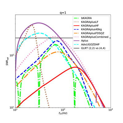
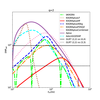
- Future prospects
Based on Ref. Baibhav:2018rfk , we discuss which noise curve for KAGRA is best for observing multiple QNMs in the ringdown data analysis. First, to estimate the SNR of the QNM GWs, we use Eq. (15) of Ref. Baibhav:2018rfk ,
| (25) |
where is the QNM amplitude related to the radiation efficiency Baibhav:2017jhs , is the sky sensitivity, is the luminosity distance, and and denote and of the () QNM.
To check the possibility of testing the no-hair theorem, we use the generalized likelihood ratio test (GLRT) Berti:2007zu where the SNR greater than can be resolved from the dominant () mode Berti:2016lat :
| (26) | |||||
| (27) |
for the () and () modes, respectively. Here, and the () mode is not excited for the equal mass case. In the following analysis, we treat the cases of and . The remnant BH spin becomes for (RIT:BBH:0198) and for (RIT:BBH:0117) Healy:2017psd ; RITcatalog .
In Fig. 9, we show the SNR of the () QNM in terms of in the case of Mpc and by using Eq. (25). We have also plotted the critical SNR evaluated by the GLRT in Eq. (27) (note the caption). It should be noted that the mass ratios of BBH estimated in the current observation are less than 666 Note that a recent observation, GW190412 LIGOScientific:2020stg has a larger mass ratio of . (the median values) GWTC1 , although unequal mass BBH give a better opportunity to test the no-hair theorem.
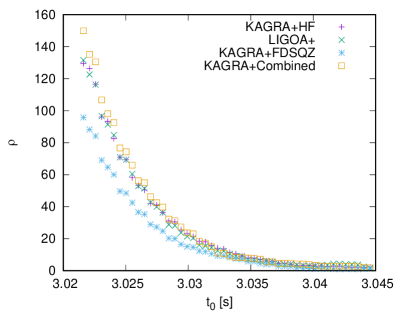
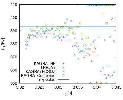
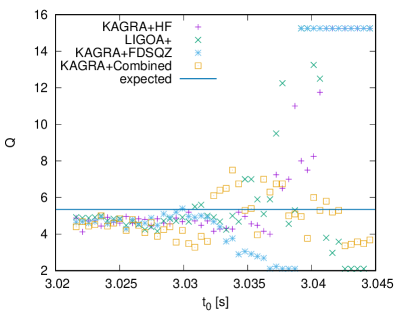
Next, we discuss effects of the shape of noise curves on the QNM parameter extraction. Figures 10 and 11 show an example only for the KAGRA+ noise curves, HF, FDSQZ, and Combined, because of the QNM frequency. In the ringdown data analysis, we can reduce the initial phase for Eq. (22) analytically. Then, we assume that the initial time as a free parameter, and search and to maximize the SNR against each . Therefore, we obtain the SNR, and for each . We see that there are some biases which depend on the detector’s configurations. It is not clear what this means, and we will give a more detailed analysis in the future Uchikata_prep .
10 Late-time cosmology
10.1 Measurement of the Hubble constant
- Scientific objective
A GW signal from a compact binary provides a unique way to measure the luminosity distance to the source. Given a source redshift, a compact binary can be utilized for measuring the cosmic expansion Schutz:1986Nature and is called the standard siren in this cosmological context Holz:2005ApJ . Particularly, the standard siren is expected to play a crucial role in measuring the Hubble constant in the next five years, using relatively nearby () GW sources, and to resolve the discrepancy problem of the Hubble constants between the cosmological measurements such as cosmic microwave background Planck2018cosmology and baryon acoustic oscillation Schoneberg:2019wmt ; Cuceu:2019for and the local measurements with Cepheid variables applied to supernovae Riess:2018byc ; Riess:2019cxk at – level. While the measurement by gravitational lensing time delay have given values consistent with that from the local measurements Collett:2019hrr ; Wong:2019kwg ; Chen:2019ejq . Recently the local measurement calibrated by the red giant branch gave a value consistent with that from the cosmological measurements Freedman:2019jwv . Therefore, pinning down the Hubble constant is an urgent issue to be solved for understanding the standard model of cosmology and could be a smoking gun of a new physics.
- Observations and measurements
The availability of the standard siren essentially depends on whether a source redshift is obtained or not. There are two ways to obtain a source redshift for an individual GW event observed by the current GW detectors: observing an EM counterpart mmaGW170817 or identifying a unique host galaxy without an EM counterpart Cutler:2009qv . If compact binaries are BNS or BH-NS binaries, one can obtain the source redshift by observing an EM counterpart that occurs coincidentally with the GW event and identifying a unique host galaxy from the sky position of the EM counterpart. For BBH, since an EM counterpart cannot be expected, redshift information needs to be obtained by identifying its host galaxy and following-up with EM spectroscopic observations. To do that, the sources must be located at lower redshifts , having high SNRs, and must be measured with good determinations of distance and sky localization Nishizawa:2016ood . Even if a unique host galaxy is not identified, information about the source redshift distribution based on galaxy catalogs is useful. By combining multiple BBH events, it is possible to select out a statistically consistent set of the cosmological parameters MacLeod:2008PRD .
Current observational constraints from one BNS merger (GW170817) and several BBH mergers with statistical redshifts are at the precisions of Abbott:2017xzu and Soares-Santos:2019irc , respectively. As the luminosity distance error is a dominant error in the measurement of the Hubble constant and degenerates with the inclination angle of a compact binary, the error in the Hubble constant can be improved by determining the inclination angle independently of the GW observation. With the help of the radio imaging observation of the superluminal jet, the inclination angle of the BNS has been constrained and the Hubble constant has been measured at the precision of Hotokezaka:2018dfi . However, these constraints are still weak to resolve the discrepancy problem and need to be improved further. To realize such a precision in the future, the modeling uncertainty of a jet, which is currently estimated to be a few percents Hotokezaka:2018dfi , also needs to be addressed.
- Future prospects
In all methods above, a good measurement of sky localization volume is essential for the identification of source redshifts and the use of the compact binaries as a cosmological probe. We estimate the measurement errors of the sky localization volume with the Fisher information matrix Nishizawa:2017nef . The sky localization volume for each compact binary is defined by Nishizawa:2016ood
| (28) |
Here is the comoving volume of a sphere with the radius . The maximum and minimum luminosity distances are determined by and , where is a fiducial source redshift and is a 2-parameter estimation error of luminosity distance. In Table 13, the sky localization volumes for various GW sources with different masses and detector networks are shown.
| source | quantile | bKAGRA | LF | HF | 40kg | FDSQZ | Combined |
|---|---|---|---|---|---|---|---|
| BBH | top 1% | 0.661 | 0.778 | 0.600 | 0.454 | 0.483 | 0.335 |
| median | 3.70 | 10.8 | 3.37 | 2.65 | 2.75 | 1.63 | |
| BBH | top 1% | 3.47 | 3.61 | 1.89 | 2.62 | 2.15 | 1.59 |
| median | 21.8 | 52.6 | 11.6 | 15.4 | 12.5 | 8.53 | |
| BH-NS | top 1% | 8.31 | 10.2 | 6.52 | 5.68 | 5.74 | 3.71 |
| median | 44.2 | 115 | 40.0 | 31.2 | 31.6 | 22.8 | |
| BNS | top 1% | 0.261 | 0.315 | 0.148 | 0.222 | 0.205 | 0.120 |
| median | 1.79 | 3.76 | 0.967 | 1.33 | 0.995 | 0.743 |
-
•
BNS and BH-NS
Based on our results of the sky localization volume, BNS are much better than BH-NS binaries. Even considering the merger rate uncertainty of BH-NS and the effect of spin precession on parameter estimation, a typical error in the Hubble constant only with BH-NS binaries is still worse than that with BNS Vitale:2018wlg . Using BNS observed by the detector network of two aLIGO and one AdV with redshift information from EM counterparts, the Hubble constant error is estimated to be Seto:2017swx ; Chen:2017rfc . With the network of the KAGRA+ near-term upgrades, the network SNR is larger by about times and the Hubble constant error is . However, the number of sources accompanying with EM counterparts is still significantly uncertain and 50 sources roughly correspond to redshift identification, which is an intermediate value of theoretical predictions Gupte:2018pht ; Howell:2018nhu ; Mogushi:2018ufy . Based on the comparison of the sky localization volume in Table 13, the improvement factors for BNS (median) are LF 0.476, 40kg 1.35, FDSQZ 1.80, HF 1.85, and Combined 2.41. The upgrades at higher frequencies lead to smaller localization volume and better sensitivity to the Hubble constant. -
•
BBH
Seen from our results of the sky localization volume, BBH are better than BBH and are easier to identify a unique host galaxy (The number density of galaxies that covers roughly 90% of the total luminosity in B-band Gehrels:2015ApJ is ) and then obtain redshift information. Assuming the number density of galaxies, top 1% events of BBH at the distance closer than can marginally identify a unique host galaxy. Extrapolating the result obtained for the bKAGRA detector network Nishizawa:2016ood to the KAGRA+ near-term upgrade networks, the Hubble constant error is . Based on the comparison of the sky localization volume in Table 13, the improvement factors for BBH (top1%) are LF 0.85, 40kg 1.46, FDSQZ 1.37, HF 1.10, Combined 1.97. For BBH, the upgrades at middle frequencies lead to smaller localization volume and better sensitivity to the Hubble constant.
In conclusion, we cannot tell which source gives better determination of the Hubble constant because of uncertainties in the merger rates of BNS and BBH, the success fraction of redshift identification, and the mass function of BBH. In addition, there would be potential contributions from systematic errors, e.g. the modeling of the EM counterparts and the calibration errors of GW detectors. Although all of these uncertainties must be reduced or improved, the standard siren has a potential to achieve the -precision measurement of the Hubble constant in the future and resolve the discrepancy problem, for which KAGRA can contribute mainly from better sky localization.
10.2 GW lensing
- Scientific objective
Gravitational lensing is a well-established subject in the EM
observation of the Universe Turner:1984ch ; Treu:2010uj . For GWs, there are controversial claims that lensing was already
observed as well from LIGO-Virgo O1/O2 detections Broadhurst:2018saj ; Broadhurst:2019ijv , while the LIGO-Virgo collaboration claimed that the
observed events are fully consistent with unlensed GWs GWTC1 . From an astrophysical viewpoint on the
lensing rate, it is unlikely that the observed events are multiple-imaged by
the stellar-mass objects Christian:2018vsi , intervening galaxy
population Ng:2017yiu , or massive galaxy clusters Smith:2017mqu .
However, for the second-generation ground-based GW detectors,
it is possible to observe several lensing events at design
sensitivity Smith:2017mqu ; Ng:2017yiu ; Li:2018prc , and almost for sure
for the third-generation detectors to detect lensed events Li:2018prc ; Christian:2018vsi . The scientific reward from lensing of GWs
is huge Finn:1995ah ; Wang:1996as ; Nakamura:1997sw , just to name a few,
ranging from probing small structures such as compact dark matter or the
primordial BHs with mass – Jung:2017flg , to discovering intermediate-mass BHs Lai:2018rto , to testing gravity theories and
cosmography Schutz:1986Nature ; Finn:1995ah .
- Observations and measurements
The detection of possible lensing events has multiple implications for
measurement. First, the lensed event is magnified in its SNR
by where is the magnification Wang:1996as , thus if
the possibility for lensing is not considered, one will underestimate its
luminosity distance by , and overestimate the masses in the source
frame with a relevant redshift rescaling thereof Wang:1996as ; Nakamura:1997sw ; Takahashi:2003ix ; Smith:2017mqu . Second, because of the magnification effect,
for events at large whose unlensed SNR is below the
detection threshold, lensing might lift it to be detectable Wang:1996as .
Therefore, lensing affects the inference on the event rate and underlying mass
distributions (and stellar evolution) of coalescing binaries. Third, if the
size of lens is comparable to or smaller than the GW
wavelength, diffraction introduces frequency-dependent time delays and
modulation of the waveform Nakamura:1997sw ; Takahashi:2003ix ; Christian:2018vsi , thus reducing the matched-filter capability if unlensed
waveforms are used as template. Fourth, for GW events with
observable EM counterparts, it is important to associate them with
each other in a convincing manner which enables tests of the speed of gravity
and inference of cosmological parameters Schutz:1986Nature ; Finn:1995ah ; Collett:2016dey ; Fan:2016swi . A precise localization with multiple detectors
helps with such statistical association.
- Future prospects
For KAGRA, it will help in localizing GW events significantly together with LIGO and Virgo observations, thus increasing the possibility to detect lensed events. No specific hardware requirement is additionally requested to achieve the gravitational lensing science goal. However, advanced data analysis including the possibility of lensing events is required. For the operation, coincident observation with LIGO and Virgo detectors is advantageous. The contribution of KAGRA data to the cooperative parameter estimation with lensing effects encoded in the waveform template will benefit the overall science output. Therefore, the same suggestion as the measurement of the Hubble constant with BBH in Sec. 10.1 is applied here.
11 Multimessenger observations
11.1 Kilonovae/Macronovae
- Scientific objective
A kilonova (a.k.a. macronova) is the emission which has been expected to be associated with a NS-NS or BH-NS merger as the consequence of the mass ejection from the system, e.g. Rosswog:1998hy ; Hotokezaka:2012ze . Since the ejected material is composed of neutron-rich matter, heavy radioactive nuclei would be synthesized in the ejecta by the so-called r-process nucleosynthesis Lattimer:1974slx ; Eichler:1989ve ; Korobkin:2012uy ; Wanajo:2014wha , and EM emission could occur by radioactive decays of heavy elements Li:1998bw ; Kulkarni:2005jw ; Metzger:2010sy ; Kasen:2013xka ; Tanaka:2013ana . Kilonova emission is expected to be bright in the optical and near infrared wavelengths and lasts for days after the merger. We note that the event rate is currently highly uncertain, while it could be if kilonovae associates with all NS-NS mergers.
The lightcurve of kilonova reflects the merger process and the late time evolution of the merger remnant Li:1998bw ; Kasen:2013xka ; Kasen:2014toa ; Barnes:2016umi ; Wollaeger:2017ahm ; Tanaka:2017qxj ; Tanaka:2017lxb . The presence of kilonova emission suggests that substantial amount of material is ejected from the system, and this gives constraints on the binary parameters by combining with a theoretical prediction obtained by numerical simulations. Furthermore, detailed properties of kilonova lightcurves, such as those brightness and color evolution, provide information of the mass and the composition of the ejected material e.g., Kasliwal:2017ngb ; Cowperthwaite:2017dyu ; Kasen:2017sxr ; Villar:2017wcc ; Perego:2017wtu ; Tanvir:2017pws ; Kawaguchi:2018ptg . Such information is useful to understand the merger process of the binary and the late-time evolution of the merger remnant as well as the chemical evolution of the universe.
- Observations and measurements
The improvement in the source localization is important to identify the host galaxy of a GW event. The source localization only by the GW data analysis would not be tight enough to uniquely identify the host galaxy even after KAGRA has joined the observation GBM:2017lvd (see Tables 4 and 5). Thus, the detection of the EM counterparts will play an important role to identify the host galaxy. In particular, searching the kilonova could have an advantage for this purpose because its emission is expected to be approximately isotropic (c.f. a short GRB). However, the detection of the kilonova will be more challenging at large distances because the kilonova will be dimmer as the distance to the event increases and the number of galaxies in the localized area significantly increases. For example, assuming the same intrinsic brightness as in GW170817, the peak r-band brightness of the kilonova would be fainter than at 200 Mpc, which is dimmer than the typical 5 limiting magnitude of 1-m class telescopes with 60 s exposure (Nissanke:2012dj, ). Thus, the improvement of the source localization via GW detection is still the key point to restrict the number of the host candidate and to achieve simultaneous detection of the kilonova of an event.
The low-latency GW alert is also a key point for the follow-up of the EM counterparts. It helps us to find the kilonova because the lightcurves, in particular in the wavelength shorter than optical bands, are most bright within a few days. Moreover, the lightcurves of the EM-counterparts at are in particular of interest. For example, in addition to the kilonova emission, the so-called cocoon emission, which is powered by internal energy deposited by relativistic jets, can contribute the early part of the lightcurve in the optical and UV wavelengths Gottlieb:2017mqv . It is pointed out that the observed data of lightcurves in can be indicative to distinguish these different components of emission Arcavi:2018mzm ; Matsumoto:2018gzy .
Tighter constraint on the inclination angle has a great impact to maximize the scientific return from the observation of the kilonova. Lightcurves of a kilonova are expected to have dependence on the observation angle Kasen:2014toa ; Perego:2017wtu ; Wollaeger:2017ahm ; Kawaguchi:2018ptg . Much more information about the property of the ejecta can be extracted if tighter constraint on the inclination angle is given. Indeed, for the recent BH-NS-like merger event GW190814 Abbott:2020khf , the constraint on the ejecta mass is obtained by the upper limits to the EM signals, while the tightness of the constraint is shown to be dependent strongly on the viewing angle Andreoni:2019qgh ; Kawaguchi:2020osi (by a factor of ).
- Future prospects
The improvements of the source localization both in speed and accuracy are crucial and would be required as the first priority for kilonova follow-up observations. The detector sensitivity should be broadband because a low frequency band is important for quick localization (early warning) and a high frequency band is important for accurate localization. According to Tables 4 and 5, the median localized area is improved by up to a factor of by including KAGRA+ in the detector network (by upgrading bKAGRA to one of KAGRA+ configurations). This enables us to search the localized fields with deeper limiting magnitudes or with less latency. For example, the EM search deeper by magnitude is in principle possible if the improvement in the localization area enabled us to spend 10 times longer exposure time. The follow-up by a 2-m class or larger class telescopes, such as Pan-STARRS (PanSTRR, ) and CTIO-Dark Energy Camera (DECam, ), are crucial for the detection for such a situation (Nissanke:2012dj, ). We also note that increase in the number of detectors with the stable operations will enhanced the chance for the multiple detectors to be operated at the same time, which is crucial for the source localization.
Tables 4 and 5 show that the determination of the inclination angle is improved by up to by including KAGRA+ in the detector network (by upgrading bKAGRA to one of KAGRA+ configurations. As mentioned above, such improvement will help us to provide the tighter constraint on ejecta properties and provide us a good opportunity to study the spatial distribution of ejecta. For example, numerical relativity simulations of a NS-binary merger (e.g., Radice:2016dwd ; Sekiguchi:2015dma ; Sekiguchi:2016bjd ; Perego:2017wtu ) predict that the typical polar opening angle of the lanthanide-rich dynamical ejecta component () is comparable to or larger than the determination error of the inclination angle for (see Tables 4 and 5). Since the presence of the lanthanide-rich material in the line of sight strongly affects the lightcurves Kasen:2014toa , the observations of kilonovae with the improved measurement of the inclination angle would enable us to examine the presence of such ejecta components.
11.2 Short gamma-ray bursts
- Scientific objective
The origin of sGRBs is a long-standing problem for more than 40 years Nakar07 ; Berger14 . A merger of BNS has been thought to be the most promising candidate Paczynski86 ; Goodman86 ; Eichler+89 , although an unequivocal evidence was missing. Although it is widely accepted that a GRB is produced by a relativistic jet with a Lorentz factor larger than , there remain unresolved issues. (1) The central engine is most likely a spinning BH surrounded by an accretion disk, while a millisecond magnetar remains a candidate. (2) The jet formation mechanism is one of the central subjects in astrophysics. It could be the Blandford-Znajek mechanism or the neutrino annihilation mechanism. For the former case, it is not known how to realize the large-scale, poloidal configuration of the magnetic field. (3) The jet composition is unknown. It is likely dominated by baryon kinetic energy or magnetic energy. (4) The emission mechanism is a puzzle. The emission radius still has approximately four order-of-magnitude uncertainty. The popular mechanism is synchrotron emission, while there is no consensus how to realize the observed spectral relations such as Amati and Yonetoku relations Amati+02 ; Yonetoku+04 . (5) The jet structure is unknown both in the radial and polar directions. The long-lasting emission following the main prompt emission such as extended emission ( s) and plateau emission ( s) suggest a long-lived central engine activity Kisaka+17 .
The detection of the GW event GW170817
GW170817PRL
and the associated EM counterparts
mmaGW170817
revolutionized the situation.
In particular, sGRB 170817A
detected two seconds ( s) after GW170817
GW170817:GRB ; GRB170817A_GBM ; GRB170817A_INT
and the following afterglows in radio to X-ray
Troja+17 ; Margutti+17 ; Haggard+17 ; Hallinan+17 ; Alexander+17 ; Lyman+18
give the first direct clues to the origin of sGRBs.
However the situation is not so simple
because sGRB 170817A was very weak
with an isotropic-equivalent energy
erg,
which is many orders of magnitude smaller than ordinary values.
On the other hand,
the afterglow observations, in particular
of superluminal motion in radio
Mooley+18b ; Ghirlanda+18
and the consistency between the spectral index
and the light curve slope after the luminosity peak
Troja+18b ; Mooley+18c ; Lamb+19 ,
strongly suggest that a relativistic jet is launched and
successfully breaks out the merger ejecta in this event
Nagakura+14 .
The jet power should be similar to those in the other normal sGRBs,
otherwise the jet cannot penetrate the merger ejecta Hamidani19 .
The most likely scenario is
that the jet is off-axis to our line-of-sight
and thereby faint in this event
IN18 ; GW170817:GRB ; Granot+17 ,
although the emission mechanism is controversial
Kasliwal+17 ; Kisaka+18 ; Nakar+18 ; Nakar19 .
The afterglow observation,
in particular the slowly-rising light curve,
is not consistent with a top-hat jet Mooley+18a ,
but for the first time strongly suggests a structured jet
Troja+18 ; Ruan+18 ; Margutti+18 ; D'Avanzo+18 ; Lazzati+18 ; Lyman+18 ; Troja+18b ; Ghirlanda+18 ; Lamb+19 .
The angular structure is also important for solving the spectral puzzles of GRB 170817A Kisaka+18 ; IN19 ; Matsumoto19a ; Matsumoto19b .
- Observations and measurements
The GW signal is basically the same as that of NS mergers with the dimensionless amplitude and a few kHz (see Sec. 4.1). The mass and mass ratio are important for revealing the jet formation mechanism since they determine the BH and disk masses after the merger.
Sky localization is essential to follow up EM counterparts LVKScenario2018 . In GW170817, the error region shrinks from 190 deg2 to 31 deg2 by adding Virgo data even though the SNR was . The survey with Subaru/Hyper Suprime-Cam (one of the most powerful telescope in the world) covered 23.6 deg2 and reached the 50% completeness magnitude of 20.6 mag Tominaga+18 . At the design sensitivities of aLIGO, AdV, and KAGRA, a typical source distance is further (or the event closer than Mpc is rare given the estimated event rate - Gpc-3 yr-1 GWTC1 ). Thus a localization error is desired to be less than deg2 and it is achievable with the detector networks including KAGRA as shown in Tables 4 and 5. Low latency should be also mandatory. In GW170817, the alert with the localization error deg2 was sent hours after the merger, although the actual observations started hours after the merger because of the interruption of the sea. In a couple of years, at least minutes or even lower latency will be realized. Ground-based detectors should try localization before the merger Cannon+12 to allow other messengers (in particular with small field of view) to observe the source at the merger time as well as possible precursor emissions.
The inclination (or viewing angle) of the merging binary is also a crucial parameter for sGRB studies. It affects all the prompt, afterglow, and kilonova emissions.
The post-merger signals are also worth to search for revealing the central engine of sGRBs Abbott+17 . They include GW emission from a hypermassive NS (or supramassive NS) and BH (see Sec. 4.3). There are many possibilities of GW emission mechanisms, such as a BH ringdown, NS quadrupolar -mode, magnetic-field-induced ellipticities, unstable bar modes, unstable -modes and so on. A possible range of GW duration is broad from s to s or even longer, as implied by long-lasting activities of sGRBs.
A magnetar giant flare is also observed as a sGRB. Some GWs are expected from giant flares (see Sec. 6.2) Ioka+00 .
Currently there is no evidence of GWs associated with giant flares Abadie+10 ,
although the -mode may not be the correct target Kashiyama+11 .
Possible candidates of giant flares include
GRB 070201 Abbott+07 ,
GRB 051103 Abadie+12
and GRB 150906B Abbott+16 .
- Future prospects
As a summary, the frequency band is required to be broadband, where the low-frequency band is important for quick localization (early warning) and the high-frequency band is important for the merger time and the post merger signals. In addition, inclination measurements are crucial. These are the same as those for a kilonova. See Sec. 11.1. As a typcial distance to GW sources gets farther, only sGRBs remain as detectable EMnetic counterparts. Collaboration with X- and gamma-ray observatories such as SVOM, Einstein Probe, HiZ-GUNDAM and CTA will become more important.
11.3 Long gamma-ray bursts
- Scientific objective
Long GRBs, whose duration is longer than about 2 s, originate in the collapse of a massive star
piran04 ; kumar15 .
Prompt gamma-ray emissions and subsequent afterglows are emitted at the head of the relativistically moving,
narrowly collimated jet toward us.
The Lorentz factor of the jet is typically larger than .
Currently the jet launch mechanism as well as the radiation process is not yet fully understood.
The central engine of the relativistic jet is also unclear, but most likely massive accretion disk around a newly formed
BH.
It has been attempted to extract the information on the dynamics and/or structure of the jet from the observed
EM emissions to tackle this problem.
However, the EM emission occurs far from the central engine, so that
previous EM observations had little direct information to answer the problem.
- Observations and measurements
In the collapsar model for long GRBs macfadyen99 , the highly spinnig core of a massive star collapses into a rotating BH with an accretion disk, or sometimes a NS, producing a relativistic jet along the rotation axis. Then, the rotating compact objects themselves emit GWs stark1985 ; kobayashi03 . This is the cases of supernovae and hypernovae. So we yield to Sec. 7.1 for more quantitative discussion. The accretion disk around the BH is massive (), so that asymmetrical blobs arise via gravitational instabilities and may be responsible for GWs kobayashi03 as well as observed gamma-ray variability. The characteristic amplitude of the GW emitted by the blob with a mass is estimated as
| (29) |
and the maximum frequency Hz, where is the distance to the source, is the BH mass, and the chirp mass .
In order to understand the jet launch mechanism, it should be clarified when and how the jet departs at the central engine. GW emission also takes place while the jet is accelerated. Such gravitational radiation has a “memory”, that is, the metric perturbation does not return to its original value at the end of the jet acceleration braginsky87 . Suppose that the mass is accelerated to a Lorentz factor . The memory GW is antibeamed (nearly isotropic) except for the on axis direction within the angle around the jet axis segalis01 ; sago04 . The characteristic amplitude is given by
| (30) |
where Hz, and is the total duration of the burst. When the acceleration takes over a time , the maximum frequency is given by . Thus, expected amplitude looks too small to bee detected. However, the amplitude may become much larger. First, the energy source is not only limited to the rest mass energy of the jet matter but also other candidates such as neutrino annihilation and magnetic field suwa09 , which can potentially be, erg. Second, the amplitude in the high-frequency range () is greatly enhanced if multiple () short bursts are taken into account sago04 . Then, the signal is about two orders of magnitude larger than that estimated in Eq. (30):
| (31) |
Once such gravitational radiation is detected, we can extract important information on the time variability and active time of the central engine as well as the jet structure.
Despite extensive searches for GWs from long GRBs,
so far the firm detection has not yet been obtained
Astone05_GRB ; Abbott05_GRB ; Aasi14_GRB ; Abbott19_GRB .
- Future prospects
For GWs from massive accretion disks or relativistic jet acceleration, observations with frequency less than 1 kHz is important. So the candidates of KAGRA+ (LF, 40kg, FDSQZ) have better sensitivities for the study of long GRBs. The local rate density of usual high-luminosity long GRBs that are detectable by gamma-ray instruments has been estimated as Gpc-3yr-1 liang07_RY . This number is for events with GRB jets toward us to emit bright gamma-rays. If the beaming factor of the jet, that is the fraction of solid angle of the gamma-ray emission to the full sky, is , then the intrinsic rate density is Gpc-3yr-1. On the other hand, the GW emission is almost isotropic. Hence the all-sky rate of the GW events within 100 Mpc is yr-1. Indeed, more frequent events in the local Universe are the low-luminosity long GRBs, the subclass of long GRBs liang07_RY . Their local rate density is two or three orders of magnitude higher than usual high-luminosity long GRBs, so that the all sky rate of nearby ( Mpc) low-luminosity long GRBs is estimated as –4 yr-1. The beaming factor for this subclass is uncertain. However, if we roughly assume , the unbeamed GW event rate is 4–40 yr-1.
The event rates of GWs sounds promising for the current GW detectors even with bKAGRA at design sensitivity. However, the memory GW is more difficult to be detected out to 100 Mpc because the matched filtering technique for a chirp signal is not available and the memory signal is more like a burst signal. In this sense, observing with more detectors is crucial and KAGRA will be able to help veto fake signals and to enhance the network sensitivity.
11.4 Fast radio bursts
- Scientific objective
Fast radio bursts (FRBs) are coherent radio transients with a duration of milliseconds. The most outstanding characteristic of FRBs is the dispersion measure (DM); they are as large as DM , indicating that the sources are at cosmological distances. A FRB is originally discovered by Lorimer et al. in 2007 2007Sci…318..777L . The number is significantly increased by wide-field-survey facilities like ASKAP and CHIME. See FRBCAT FRBCAT for an updated catalog.
It is now known that a fraction (roughly ) of the FRBs are repeating. The differences between repeating and non-repeating FRBs are still under debate. Host galaxies have been reported for a few FRBs; both for repeating and non-repeating ones. There is a diversity in the host galaxies; the host of FRB 121102 is a dwarf star forming galaxy while other host galaxies are medium-sized less-active galaxies. No multi-messenger counterpart has been reported.
The origin of FRB is still not known, and the emission mechanism is rather uncertain.
Given the similarities between FRB and some transient phenomena from Galactic young NSs, e.g., giant radio pulses from the Crab pulsar and magnetar giant flares, the young NS models have been most intensively investigated. See, e.g. 2017ApJ…839L…3K and references therein. For a GW from a young NS, see Secs. 6.2 and 6.3.
On the other hand, the most testable and interesting possibility for KAGRA and other ground-based interferometers would be the coalescing BNS model 2013PASJ…65L..12T ; FRBs could be produced just before the merger, a fraction of the orbital energy being extracted by magnetic braking. Simultaneous detection of a GW and an FRB is the straightforward way to test this scenario.
- Observations and measurements
If a FRB is observed with a GW, the source will be determined. In general, arrival timing of the FRB relative to the GW is useful; the FRB will be emitted, say milliseconds after the the GWs.
The timing of the FRB emission should be closely connected to the emission mechanism; information on the physical condition of the NS magnetosphere can be obtained.
- Future prospects
Ongoing and upcoming radio surveys could detect FRBs per year (see e.g., (2017ApJ…844..140C, )), providing more opportunities to conduct multi-messenger observations. One can search the GW counterpart of known FRBs; in addition to Galactic young NSs, we can select relatively close extragalactic targets based on their DMs. Conversely, GW detectors could in principle give an alert to radio telescopes. Since the field of view of radio telescopes is relatively small (e.g., 0.1 deg for Parkes), a better sky localization with KAGRA is, as always, crucial.
12 Others
12.1 Cosmic strings
- Scientific objective
Cosmic strings are one-dimensional cosmological defects that are predicted to form under phase transitions in the early Universe Kibble76 . More recently, it has been recognized that cosmological models based on the string theory also result in string forming and growing to cosmic scales Sarangi02 ; Jeannerot03 . A cosmic string is characterized by its tension, which is linked to the energy scale of the Universe when it is formed. Searching for cosmic strings will thus allow us to investigate the early time of the Universe that has never been probed before.
- Observations and measurements
A promising observational signature of cosmic strings is their gravitational radiation from loops Damour00 ; Damour01 ; Damour05 . Loops can form through a process called intercommutation, in which two strings change partners upon encounter. An intercommutation of a loop by itself or of two strings on two points creates a loop, which oscillates and radiates their energy by GWs. Special points that are occasionally formed on loops, called cusps and kinks, are the important targets for GW detectors. Cusps are points on a loop that accompany large Lorentz boosts, and kinks are discontinuities on the tangent vectors of a loop Vilenkin00 . Another interesting GW source is kinks on infinitely long cosmic strings Matsui:2016xnp ; Matsui:2019obe , which are produced when two strings intersect. As the string network evolves with continuous intersections, a number of small kinks accumulate on infinite strings and their propagation and collisions generate GW bursts. Although the strain amplitude of each GW burst is small, a number of overlapped bursts due to the high event rate generate a GW background with a large amplitude, enough to be tested by the ground-based experiments.
Search for cosmic strings have been conducted in the past, using data from LIGO and Virgo detectors Abbott09 ; Aasi14 ; Abbott18 . These works have done two searches, a template-based matched-filtering search for individual burst signals (from cusps and kinks), and a search for the stochastic background generated by an overlapping population of these bursts. These searches have given constraints on the string parameters (e.g. tension) and models on the distribution of these loops in the Universe. The constraints depend on models of the probability distribution on the loop size. The searches using aLIGO’s O1 data Abbott18 yielded a constraint of for a simple loop model first developed in Vilenkin00 ; Damour01 .
GW emission from these features are predicted to be linearly polarized, and have a power-law frequency spectrum of index for cusps and for kinks Damour01 . The amplitude depends on the tension and size of the loop, as well as the distance to the loop. The spectrum also is considered to have a high-frequency cutoff due to the beamed nature of the signal. The high-frequency cutoff can take arbitrary values, but as bursts with higher frequency cutoff are more beamed Damour01 , bursts with lower high-frequency cutoffs can be seen more frequently than those with higher high-frequency cutoffs.
- Future prospects
Due to the power-law nature, the signals from cosmic string bursts generally have higher amplitudes in low frequencies. Hence the sensitivity to string signals will be most enhanced by improving the lower frequency band Abbott18 . By defining the SNR ratio for the configurations and where is defined in Eq. (5) and a similar equation holds for the configuration, We can quantitatively compare performances of various configurations of possible KAGRA upgrades. For a cosmic string cusp, the amplitude is proportional to . If we take the high frequency cutoff at Hz, the SNR ratios from bKAGRA to KAGRA+ for a GW burst from a cosmic string cusp are LF 5.46, 40kg 1.54, FDSQZ 1.19, HF 0.39, Combined 2.82. Also significant sensitivity improvements in low frequencies are anticipated in the upgrades of aLIGO and AdV or the Einstein Telescope. Furthermore, because the string bursts are linearly polarized, using the information of polarization can be crucial for differentiating these signals from noise. This can be sufficiently done with a KAGRA detector in collaboration with the LIGO and Virgo detectors.
12.2 Black-hole echoes
- Scientific objective
The BH information loss paradox is a long standing problem. The problem looks complicated, but the rough idea can be captured in the following way. Our assumptions are the followings:
-
1.
Hawking evaporation can be described by a semi-classical picture. Namely, it can be described by the standard field theory in curved spacetime. This means that BHs radiate like a black body at the Hawking temperature , where is the surface gravity. In the case of a Schwarzschild BH, the surface gravity is given by with being the horizon radius. This emitted radiation is perfectly entangled with the internal state of the BH. It would not be so difficult to convince yourself that this argument is likely. If we simply consider the evolution of initially pure quantum state, it remains so in the ordinary field theory. So, if the emitted radiation looks thermal, this thermal nature is obtained as a result of integrating out some unobserved degrees of freedom. In the case of a BH spacetime, these hidden degrees of freedom are inside the BH horizon.
-
2.
BH entropy is bounded by the area of the BH, i.e., , where is the area of the BH and is Newton’s constant. Under the assumption that this bound is saturated, the BH thermodynamics holds.
These assumptions can be easily seen to be inconsistent. Let us consider a stationary process containing a BH emitting the Hawking radiation. To make it stationary, we keep throwing some matter continuously down into the BH. Then, in a mean time the total entropy of the emitted radiation exceeds . However, the internal state entangled with the emitted radiation should also have the same amount of entropy. Since the spacetime is stationary with an apparent horizon, no information can go out from the inside. This would contradict with the claim that the BH entropy is bounded by .
To resolve the contradiction mentioned above, some of assumptions must be violated. An easy way is to abandon the assumption (2). However, many people believe that the BH entropy identified with its area is not just a theoretical illusion but has a deep physical meaning. As far as we wish to keep the assumption (2), we would be requested to abandon the assumption (1). One possibility is that the Hawking radiation is wrong. However, this is unlikely, although it is true that the explicit calculation of the Hawking radiation based on the field theory in curved spacetime is given only in weak coupling perturbative calculations. Then, at first glance radical but in a certain sense most conservative idea to resolve the contradiction will be to abandon the semi-classical picture. From the point of view of relativity, the horizon is not a special surface at all, unless we care about the global structure of the spacetime. Therefore it is difficult to imagine that something unusual happen particularly on the horizon. However, if we trace back the quanta emitted as the Hawking radiation, it infinitely blue-shifts in the near horizon limit. Hence, field theoretically the horizon might be somehow special, although the argument sounds a little acausal.
From the discussion mentioned above, it would be well-motivated to doubt if the physics describing the region close to the BH horizon
might be significantly modified from our familiar low energy physics.
One simple but radical possibility is that the BH horizon is
covered by a wall which reflects all the low energy excitations
including GWs. Ordinary matter whose energy scale is much higher
than the energy of the typical gravitons excited in the binary system
will be absorbed by BHs,
while the quanta whose energy is comparable or
lower than , i.e., whose wavelength is as long as the BH size,
are selectively reflected by the wall. Interestingly, this critical energy scale
also follows if we assume that the
BH area is quantized by the Planck length
squared Bekenstein:1974jk ; Mukhanov:1986me ; Barcelo:2017lnx .
- Observations and measurements
It is difficult to predict the exact waveform of the expected echoes, since the theoretical background is not so sound. What we can expect generically is the repetition of signals similar to the ringdown signal after merger with an equal time interval. Here, the uncertainties are in the boundary condition at the wall and the wall location. One possible ansatz about the properties of the wall is that the reflection rate at the wall is unity and the wall is placed at about a Planck distance from the horizon. Furthermore, we also need to make an assumption about the phase shift at the reflection. One simple assumption is that the phase shift is frequency independent or the frequency dependence is sufficiently weak. Under such an assumption, we could construct a template by solving the master equation for BH perturbation Nakano .
There was a claim that some echo signal has been already detected Abedi .
However, very simple repetition of the same waveform was assumed in their analysis.
Such an analysis is an interesting trial, but it is difficult to invent a theoretical model that
supports that simple-minded assumption. In fact, our reanalysis indicates that
the significance of the echo signal does not survive once we replace the
template with a little more realistic one Uchikata:2019frs , i.e., the reflection rate at the angular momentum barrier calculated by using the BH perturbation theory is employed.
However, it is also true that the signal claimed in Abedi does not disappear just by increasing the number of BH merger events including the events from LIGO/Virgo O2 observing run.
- Future prospects
Definitely, as the number of events increases, the nature of the signal that seem to be existing will be uncovered in near future. In order to discriminate the real signal coming from the sky from the unidentified noise of detectors correlated with GW events, it would be better to analyze the data from completely different detectors which have a similar sensitivity. In this sense it is quite interesting to analyse the data obtained by Virgo and KAGRA in the same manner.
13 Conclusion
In this article we have reviewed scientific cases available with the second-generation ground-based detectors including aLIGO, AdV, the baseline KAGRA (bKAGRA) and their future upgrades, A+, AdV+, and KAGRA+, respectively, and discuss KAGRA’s scientific contributions to the global detector networks composed of the detectors above. For compact binaries composed of stellar-mass BHs and/or NSs, at least three detectors are necessary to localize sources and more detectors including KAGRA is preferable to obtain smaller sky areas to be searched. This is also true for sciences based on these binaries such as the tests of gravity (except for BH ringdown), the measurement of the Hubble constant, GW lensing, the measurement of EOS of a NS, and the multimessenger observations of short-gamma ray bursts and kilonovae. On the other hand, the discovery of new GW sources such as binary IMBHs, supernovae, magnetors, isolated pulsars, and low-mass X-ray binaries can be done with a single detector, though multiple detectors are preferable for events detected only by GWs. Therefore, for these sources, the higher duty cycle of a detector network is more important not to miss signals during detector down times. In summary, KAGRA will be able to contribute to broad science topics and play an important role in joint observations by the global detector networks.
Acknowledgment
This work was supported by MEXT, JSPS Leading-edge Research Infrastructure Program, JSPS Grant-in-Aid for Specially Promoted Research 26000005, JSPS Grant-in-Aid for Scientific Research on Innovative Areas 2905: JP17H06358, JP17H06361 and JP17H06364, JSPS Core-to-Core Program A. Advanced Research Networks, JSPS Grant-in-Aid for Scientific Research (S) 17H06133, the joint research program of the Institute for Cosmic Ray Research, University of Tokyo, National Research Foundation (NRF) and Computing Infrastructure Project of KISTI-GSDC in Korea, Academia Sinica (AS), AS Grid Center (ASGC) and the Ministry of Science and Technology (MoST) in Taiwan under grants including AS-CDA-105-M06, Advanced Technology Center (ATC) of NAOJ, Mechanical Engineering Center of KEK, the LIGO project, and the Virgo project.
References
- (1) T. Akutsu, et al. (KAGRA collaboration), in preparation as the series of article. Overview of KAGRA: Future plans.
- (2) J. Aasi et al., (LIGO Scientific Collaboration, Advanced VIRGO), Class. Quant. Grav. 32, 074001 (2015).
- (3) F. Acernese et al., Class. Quant. Grav. 32, 024001 (2015).
- (4) B. P. Abbott et al.(LIGO Scientific and Virgo Collaboration), \PRX9,031040,2019
- (5) B. P. Abbott et al.(LIGO Scientific and Virgo Collaboration), \PRL119,161101,2017
- (6) B. P. Abbott et al.(LIGO Scientific and Virgo Collaboration), \PRL116,061102,2016
- (7) B. P. Abbott et al.(LIGO Scientific and Virgo Collaboration), \PRL116,241103,2016
- (8) B. P. Abbott et al.(LIGO Scientific and Virgo Collaboration), \PRL118, 221101 ,2017
- (9) B. P. Abbott et al.(LIGO Scientific and Virgo Collaboration), Astrophys. J. Lett. 851, L35 (2017).
- (10) B. P. Abbott et al.(LIGO Scientific and Virgo Collaboration), \PRL119,141101,2017
- (11) B. P. Abbott, et al. Astrophys. J. Lett. 848, L12 (2017).
- (12) J. Miller et al., \PRD91,062005,2015
- (13) J. Degallaix for the Virgo Collaboration, Advanced Virgo+ preliminary studies, VIR-0300A-18 (2018).
- (14) B. P. Abbot et al., Liv. Rev. Rel. 21, 3 (2018).
- (15) T. Akutsu et al., (KAGRA collaboration) Nat. Astron. 3, 35 (2019).
- (16) Y. Michimura et al., \PRD102,022008,2020
- (17) B. P. Abbott et al.(LIGO Scientific and Virgo Collaboration), Astrophys. J. Lett. 818, L22 (2016).
- (18) K. Belczynski, T. Bulik and B. Rudak, Astrophys. J. Lett. 608, L45 (2004).
- (19) M. Dominik, K. Belczynski, C. Fryer, D. E. Holz, E. Berti, T. Bulik, I. Mandel and R. O’Shaughnessy, Astrophys. J. 759, 52 (2012).
- (20) K. Belczynski, D. E. Holz, T. Bulik and R. O’Shaughnessy, Nature 534, 512 (2016).
- (21) M. Mapelli, Mon. Not. R. Astron. Soc. 459, 3432 (2017).
- (22) S. F. Portegies Zwart and S. L. W. McMillan, Astrophys. J. Lett. 528, L17 (2000).
- (23) R. M. O’Leary, B. Kocsis and A. Loeb, Mon. Not. R. Astron. Soc. 395, 2127 (2009).
- (24) T. Chiba and S. Yokoyama, Prog. Theor. Exp. Phys. 2017, 083E01 (2017).
- (25) V. De Luca, V. Desjacques, A. Malhotra and A. Riotto, J. Cosmol. Astropart. Phys. 05, 018 (2019).
- (26) T. Harada, Y. Chul-Moon, K. Kohri, and K. Nakao, \PRD96,083517,2017 Erratum: ibid. 99, 069904 (2019).
- (27) C. L. Rodriguez, C.-J. Haster, S. Chatterjee, V. Kalogera and F. A. Rasio, Astrophys. J. Lett. 824, L8 (2016).
- (28) F. Antonini and F. A. Rasio, Astrophys. J. 831, 187 (2016).
- (29) N. C. Stone, B. D. Metzger and Z. Haiman, Mon. Not. R. Astron. Soc. 464, 946 (2017).
- (30) Y.-B. Bae, C. Kim, H. M. Lee Mon. Not. R. Astron. Soc. 440, 2714 (2014).
- (31) D. Park, C. Kim, H. M. Lee, Y.-B. Bae, K. Belczynski Mon. Not. R. Astron. Soc. 469, 4665 (2017).
- (32) T. Kinugawa, K. Inayoshi, K. Hotokezaka, D. Nakauchi and T. Nakamura, Mon. Not. R. Astron. Soc. 442, 2963 (2014).
- (33) T. Hartwig, M. Volonteri, V. Bromm, R. S. Klessen, E. Barausse, M. Magg and A. Stacy, Mon. Not. R. Astron. Soc. 460, L74 (2016).
- (34) K. Inayoshi, K. Kashiyama, E. Visbal and Z. Haiman, Mon. Not. R. Astron. Soc. 461, 2722 (2016).
- (35) K. Inayoshi, R. Hirai, T. Kinugawa and K. Hotokezaka, Mon. Not. R. Astron. Soc. 468, 5020 (2017).
- (36) D. Kushnir, M. Zaldarriaga, J. A. Kollmeier and R. Waldman, Mon. Not. R. Astron. Soc. 462, 844 (2016).
- (37) C. L. Rodriguez, M. Zevin, C. Pankow, V. Kalogera and F. A. Rasio Astrophys. J. Lett. 832, L2 (2016).
- (38) K. Hotokezaka and T. Piran, Astrophys. J. 842, 111 (2017).
- (39) T. Janka Mon. Not. R. Astron. Soc. 434, 1355 (2013).
- (40) I. Mandel Mon. Not. R. Astron. Soc. 456, 578 (2016).
- (41) E. S. Phinney, arXiv:astro-ph/0108028.
- (42) B. P. Abbott et al.(LIGO Scientific and Virgo Collaboration), \PRL116,131102,2016
- (43) B. Carr, F. Kühnel and M. Sandstad, \PRL94,083504,2016
- (44) M. Sasaki, T. Suyama, T. Tanaka and S. Yokoyama, \PRL117,061101,2016
- (45) M. Sasaki, T. Suyama, T. Tanaka, and S. Yokoyama, Class. Quant. Grav. 35, 063001 (2018).
- (46) K. A. Postnov and L. R. Yungelson, Liv. Rev. Rel. 17, 3 (2014).
- (47) M. J. Benacquista, Liv. Rev. Rel. 5, 2 (2002).
- (48) L. Pekowsky, J. Healy, D. Shoemaker, P. Laguna \PRD87,084008,2013
- (49) B. P. Abbott et al.(LIGO Scientific and Virgo Collaboration), arXiv:2004.08342.
- (50) J. M. Bardeen et al., Astrophys. J. 178, 347 (1972).
- (51) S. F. Portegies Zwart and S. L. W. McMillan, Astrophys. J. 576, 899 (2002).
- (52) M. Freitag, M. A. Gürkan and F. A. Rasio, Mon. Not. R. Astron. Soc. 368, 141 (2006).
- (53) P. Amaro-Seoane and L. Santamaría, Astrophys. J. 722, 1197 (2010).
- (54) G. Fragione, I. Ginsburg and B. Kocsis, Astrophys. J. 856, 92 (2018).
- (55) H.-a. Shinkai, N. Kanda and T. Ebisuzaki, Astrophys. J. 835, 276 (2017).
- (56) P. Amaro-Seoane, \PRD98,063018,2018
- (57) M. A. Gürkan, J. M. Fregeau and F. A. Rasio, Astrophys. J. Lett. 640, L39 (2006).
- (58) S. Hirano, T. Hosokawa, N. Yoshida, H. Umeda, K. Omukai, G. Chiaki and H. W. Yorke, Astrophys. J. 780, 60 (2014).
- (59) A. Stacy and V. Bromm, Mon. Not. R. Astron. Soc. 433, 1094 (2013).
- (60) H. Susa, K. Hasegawa and N. Tominaga, Astrophys. J. 792, 32 (2014).
- (61) K. Inayoshi, Z. Haiman, Mon. Not. R. Astron. Soc. 445, 1549 (2014).
- (62) M. C. Miller et al., Int. J. Mod. Phys. D 13, 1 (2004).
- (63) D. A. Brown et al., \PRL99,201102,2007
- (64) E. Berti et al., \PRD71,084025,2005
- (65) S. Isoyama et al., Prog. Theor. Exp. Phys. 2018, 073E01 (2018).
- (66) A. Ori et al., \PRD62,124022,2000
- (67) E. Berti et al., \PRD73,064030,2006
- (68) E. A. Huerta et al., \PRD83,044020,2011
- (69) M. C. Miller, Class. Quant. Grav. 26, 094031 (2009).
- (70) T. M. Tauris et al., Astrophys. J. Lett. 846, L170 (2017).
- (71) M. Chruslinska, K. Belczynski, J. Klencki1, M. Benacquista, Mon. Not. R. Astron. Soc. 474, 2937 (2018).
- (72) D. Pooley et al., Astrophys. J. Lett. 591, L131 (2019)..
- (73) J. M. Weisberg, D. J. Nice, J. H. Taylor, Astrophys. J. 722, 1030 (2010).
- (74) P. C. Peters, \PRB136,1224,1964
- (75) F. Özel and P. Freire, Annu. Rev. Astron. Astrophys, 54, 401 (2016).
- (76) B. P. Abbott et al.(LIGO Scientific and Virgo Collaboration), Astrophys. J. Lett. 896, L44 (2020).
- (77) N. Pol, M. McLaughlin, D.R. Lorimer, Astrophys. J. 870, 71 (2019).
- (78) R. N. Manchester, G. B. Hobbs, A. Teoh and M. Hobbs, Astrophys. J. 129, 1993 (2005).; ATNF Pulsar Catalogue webpage, http://www.atnf.csiro.au/research/pulsar/psrcat/
- (79) B. P. Abbott et al.(LIGO Scientific and Virgo Collaboration), \PRX9,011001,2019
- (80) J. M. Lattimer and M. Prakash, Phys. Rept. 621, 127 (2016).
- (81) E. E. Flanagan and T. Hinderer, \PRD77,021502,2008
- (82) T. Hinderer, Astrophys. J. 677, 1216 (2008).
- (83) T. Damour, A. Nagar and L. Villain, Phys. Rev. D 85, 123007 (2012) \PRD85,123007,2012
- (84) L. Wade, J. D. E. Creighton, E. Ochsner, B. D. Lackey, B. F. Farr, T. B. Littenberg and V. Raymond, \PRD89,103012,2014
- (85) T. Hinderer, B. D. Lackey, R. N. Lang and J. S. Read, \PRD81,123016,2010
- (86) K. Hotokezaka, K. Kyutoku, H. Okawa, M. Shibata and K. Kiuchi, \PRD83,124008,2011
- (87) A. Buonanno, B. R. Iyer, E. Ochsner, Y. Pan and B. S. Sathyaprakash, \PRD80,084043,2009
- (88) L. Blanchet, Living Rev. Rel. 17, 2 (2014).
- (89) T. Dietrich, S. Bernuzzi and W. Tichy, \PRD96,121501,2017
- (90) K. Yagi and N. Yunes, Phys. Rept. 681, 1 (2017)
- (91) B. P. Abbott et al.(LIGO Scientific and Virgo Collaboration), \PRL121,161101,2018
- (92) W. Kastaun and F. Ohme, \PRD100,103023,2019
- (93) B. P. Abbott et al.(LIGO Scientific and Virgo Collaboration), Class. Quant. Grav. 37, 045006 (2020).
- (94) H. Mueller and B. D. Serot, Nucl. Phys. A 606, 508 (1996).
- (95) S. De, D. Finstad, J. M. Lattimer, D. A. Brown, E. Berger and C. M. Biwer, \PRL121,091102,2018 Erratum: ibid. 121, 259902 (2018).
- (96) C. D. Capano et al., Nature Astron. 4:625 (2020).
- (97) T. Narikawa, N. Uchikata, K. Kawaguchi, K. Kiuchi, K. Kyutoku, M. Shibata and H. Tagoshi, arXiv:1910.08971.
- (98) K. Kiuchi, K. Kawaguchi, K. Kyutoku, Y. Sekiguchi, M. Shibata and K. Taniguchi, \PRD96,084060,2017
- (99) K. Kawaguchi, K. Kiuchi, K. Kyutoku, Y. Sekiguchi, M. Shibata and K. Taniguchi, \PRD97,044044,2018
- (100) T. Dietrich, A. Samajdar, S. Khan, N. K. Johnson-McDaniel, R. Dudi and W. Tichy, \PRD100,04403,2019
- (101) B. Margalit and B. D. Metzger, Astrophys. J. Lett. 850, L19 (2017).
- (102) A. Bauswein, O. Just, H. T. Janka and N. Stergioulas, Astrophys. J. Lett. 850, L34 (2017).
- (103) M. Ruiz, S. L. Shapiro and A. Tsokaros, \PRD97,021501(R),2018
- (104) E. Annala, T. Gorda, A. Kurkela and A. Vuorinen, \PRL120,172703,2018
- (105) E. P. Zhou, X. Zhou and A. Li, \PRD97,083015,2018
- (106) F. J. Fattoyev, J. Piekarewicz and C. J. Horowitz, \PRL120,172702,2018
- (107) V. Paschalidis, K. Yagi, D. Alvarez-Castillo, D. B. Blaschke and A. Sedrakian, \PRD97,084038,2018
- (108) R. Nandi and P. Char, Astrophys. J. 857, 12 (2018).
- (109) E. R. Most, L. R. Weih, L. Rezzolla and J. Schaffner-Bielich, \PRL120,261103,2018
- (110) C. Raithel, F. Özel and D. Psaltis, Astrophys. J. Lett. 857, L23 (2018).
- (111) P. Landry and R. Essick, \PRD99,084049,2019
- (112) L. Baiotti, Prog. Part. Nucl. Phys., 109, 103714 (2019).
- (113) K. Takami, L. Rezzolla and L. Baiotti, \PRD91,064001,2015
- (114) A. Akmal, V. R. Pandharipande and D. G. Ravenhall, \PRC58,1804,1998
- (115) F. Douchin and P. Haensel, Astron. Astrophys. 380, 151 (2001).
- (116) T. Narikawa, N. Uchikata, K. Kawaguchi, K. Kiuchi, K. Kyutoku, M. Shibata and H. Tagoshi, Phys. Rev. Research. 1, 033055 (2019)
- (117) L. Baiotti and L. Rezzolla, RPPh, 80, 096901 (2017).
- (118) M. D. Duez and Y. Zlochower, Rep. Prog. Phys., 82, 016902 (2019).
- (119) V. Paschalidis and N. Stergioulas, Liv. Rev. Rel. 20, 7 (2017).
- (120) K. Takami, L. Rezzolla and L. Baiotti, \PRL113,091104,2014
- (121) F. Maione, R. De Pietri, A. Feo and F. Löffler, \PRD96,063011,2017
- (122) M. Breschi, S. Bernuzzi, F. Zappa, M. Agathos, A. Perego, D. Radice and A. Nagar, \PRD100,104029,2019
- (123) A. Bauswein and H.-T. Janka, \PRL108,011101,2012
- (124) S. Bose, K. Chakravarti, L. Rezzolla, B. S. Sathyaprakash and K. Takami, \PRL120,031102,2018
- (125) K. Chatziioannou, J. A. Clark, A. Bauswein, M. Millhouse, T. B. Littenberg, and N. Cornish, \PRD96,124035,2017
- (126) A. Torres-Rivas, K. Chatziioannou, A. Bauswein and J. A. Clark, \PRD99,044014,2019
- (127) L. R. Weih, M. Hanauske and L. Rezzolla, \PRL124,171103,2020
- (128) A. Bauswein, S. Blacker, V. Vijayan, N. Stergioulas, K. Chatziioannou J. Clark N. Bastian D. B. Blaschke M. Cierniak and T. Fischer, arXiv:2004.00846.
- (129) L. Baiotti, B. Giacomazzo and L. Rezzolla, \PRD78,084033,2008
- (130) L. Rezzolla, B. Giacomazzo, L. Baiotti, L. Granot, C. Kouveliotou and M.A. Aloy, Astrophys. J. Lett. 732, L6 (2011).
- (131) K. Kiuchi,Y. Sekiguchi, K. Kyutoku, M. Shibata, K. Taniguchi and T. Wada, \PRD92,064034,2015
- (132) D. Radice, A. Perego, K. Hotokezaka et al., Astrophys. J. 869, 130 (2018).
- (133) R. P. Kerr, \PRL11,237,1963
- (134) M. H. P. M. van Putten, Science 284, 115 (1999).
- (135) M. H. P. M. van Putten, M. Della Valle, and A. Levinson, Astrophys. J. 876, L2 (2019).
- (136) R. De Pietri, A. Drago, A. Feo, et al., Astrophys. J. 881, 122 (2019).
- (137) J. Klimo, M. Veselsky, G. A. Souliotis, A. Bonasera, Nucl. Phys. A, 992, 121640 (2019).
- (138) P. Haensel, J. L. Zdunik, M. Bejger et al., A&A, 502, 605 (2009).
- (139) V. Connaughton, GCN, 21505 (2017).
- (140) V. Savchenko et al., Astrophys. J. Lett. 848, L15 (2017).
- (141) K. P. Mooley, A. T. Deller, O. Gottlieb et al., Nature 554, 207 (2018).
- (142) K. P. Mooley, A. T. Deller, O. Gottlieb et al., Nature 561, 355 (2018).
- (143) C. Cutler and K. S. Thorne, arXiv:gr-qc/0204090.
- (144) R. A. Hulse and J. H. Taylor, Astrophys. J. Lett. 195, L51 (1975).
- (145) K. W. Weiler and N. Panagia, A&A, 70, 419 (1978).
- (146) B. P. Abbott et al., Astrophys. J. Lett. 848, L13 (2017).
- (147) B. P. Abbott et al., Astrophys. J. 875, 160 (2019).
- (148) L. Sun and A. Melatos, \PRD99,123003,2019
- (149) R. Gill, A. Nathanail, and L. Rezzolla, Astrophys. J. 876, 139 (2019).
- (150) S. J. Smartt, T.-W. Chen, A. Jerkstrand et al., Nature 551, 75 (2017).
- (151) E. Pian, P. D’Avanzo, S. Benetti et al., Nature 551, 67 (2017).
- (152) M. Lucca and L. Sagunski, JHEAp 27, 33 (2020)
- (153) D. Pooley, P. Kumar, J. C. Wheeler, B. Grossan, Astrophys. J. Lett. 859, L23 (2018).
- (154) M. H. P. M. van Putten, C. Guidorzi, and F. Frontera Astrophys. J. 786, 146 (2014).
- (155) M. H. P. M. van Putten, PTEP, 093F01 (2017).
- (156) M. H. P. M. van Putten and M. Della Valle, Mon. Not. R. Astron. Soc. 482, L46 (2019).
- (157) B. P. Abbott et al., Astrophys. J. Lett. 851, L16 (2017).
- (158) M. H. P. M. van Putten, A. Levinson, F. Frontera, C. Guidorzi, L. Amati, and M. Della Valle, EPJ Plus, 134, 547 (2019).
- (159) J.-E. Heo, S. Yoon,D.-S Lee, et al., New Astronomy 42, 24 (2016).
- (160) S. Ando, B. Baret, I. Bartos, et al., Rev. Mod. Phys. 85 (2013).
- (161) J. Aasi, B.P. Abbott, T. Abbott, et al., \PRD89,122004,2014
- (162) L. Amati,P. O’Brian,D. Götz, et al., Adv. Space Sc., 62, 191 (2018).
- (163) G. Stratta,R. Ciolfi,L. Amati, et al., Adv. Space Sc., 62, 662 (2018).
- (164) K. Riles, Modern Physics Letters A 32, 1730035-685 (2017).
- (165) G. Ushomirsky et al., Mon. Not. R. Astron. Soc. 319, 902 (2000).
- (166) L. Bildsten, Astrophys. J. Lett. 501, L89 (1998).
- (167) A. Mukherjee et al., \PRD97,043016,2018
- (168) G. D. Meadors et al., \PRD95,042005,2017
- (169) B. P. Abbott et al., Astrophys. J. 847, 47 (2017).
- (170) B. P. Abbott et al., \PRD95,122003,2017
- (171) B. P. Abbott et al., \PRD100,122002,2019
- (172) L. J. Kaluzienski et al., Astrophys. J. 241, 779 (1980).
- (173) C. Messenger et al., \PRD92,023006,2015
- (174) G. D. Meadors et al., \PRD97,044017,2018
- (175) C. Dreissigacker et al., \PRD100, 044009, 2019
- (176) R. Smits, S. J. Tingay, N. Wex, M. Kramer and B. Stappers, Astronomy & Astrophysics 528, A108 (2011).
- (177) K. Glampedakis and L. Gualtieri, Astrophys. Space Sci. Libr. 457, 673 (2018).
- (178) M. Sieniawska and M. Bejger, Universe 5, 217, (2019).
- (179) B. P. Abbott et al.(LIGO Scientific and Virgo Collaboration), Astrophys. J. 875, 122 (2019).
- (180) K. Ono, K. Eda, and Y. Itoh, \PRD91,084032,2015
- (181) B. P. Abbott et al.(LIGO Scientific and Virgo Collaboration), Astrophys. J. 851, 71 (2017).
- (182) B. P. Abbott et al.(LIGO Scientific and Virgo Collaboration), Astrophys. J. 879, 10 (2019).
- (183) B. P. Abbott et al.(LIGO Scientific and Virgo Collaboration), \PRL120,031104,2018
- (184) N. K. Johnson-McDaniel and B. J. Owen, \PRD88,044004,2013
- (185) N. K. Johnson-McDaniel, \PRD88,044016,2013
- (186) Matthew Pitkin, Mon. Not. R. Astron. Soc. 415, 1849 (2011).
- (187) G. L. Israel et al., Astrophys. J. Lett. 628, L53 (2005).
- (188) K. Ioka, Mon. Not. R. Astron. Soc. 327, 639 (2001).
- (189) A. Corsi et al., \PRD83,104014,2011
- (190) Y. Levin et al., Mon. Not. R. Astron. Soc. 418, 659 (2011).
- (191) B. Zink et al., \PRD85,1002030,2012
- (192) B. P. Abbott et al.(LIGO Scientific Collaboration)\PRD76,062003,2007
- (193) B. P. Abbott et al.(LIGO Scientific Collaboration)Astrophys. J. 874, 163 (2019).
- (194) K. Kokkotas et al., Liv. Rev. Rel. 2, 2 (1999).
- (195) N. Andersson et al., \PRL77,4134,1996
- (196) N. Andersson et al., Mon. Not. R. Astron. Soc. 299, 1059 (1998).
- (197) L. S. Finn Mon. Not. R. Astron. Soc. 227, 265 (1987).
- (198) H. Sotani et al., \PRD65,024010,2001
- (199) G. Miniutti et al., Mon. Not. R. Astron. Soc. 338, 389 (2003).
- (200) H. Sotani et al., \PRD83,024014,2011
- (201) R. Reisenegger et al., Astrophys. J. 395, 240 (1992).
- (202) V. Ferrari et al., Class. Quant. Grav. 24, 5093 (2007).
- (203) A. Passamonti et al., Mon. Not. R. Astron. Soc. 455, 1489 (2016).
- (204) N. Andersson Astrophys. J. 502, 708 (1998).
- (205) J. L. Friedman et al., Astrophys. J. 502, 714 (1998).
- (206) P. Arras et al., Astrophys. J. 591, 1129 (2003).
- (207) E. Gaertig et al., \PRL107,101102,2011
- (208) H. Sotani et al., \PRD94,044043,2016
- (209) H. Sotani et al., \PRD96,063005,2017
- (210) V. Morozova et al., Astrophys. J. 861, 10 (2018).
- (211) H. Sotani et al., \PRD99,123024,2019
- (212) H. Sotani, K. Sumiyoshi \PRD100,083008,2019
- (213) A. Torres-Forné et al., Mon. Not. R. Astron. Soc. 474, 5272 (2018).
- (214) A. Torres-Forné et al., Mon. Not. R. Astron. Soc. 482, 3967 (2019).
- (215) B. W. Grefenstette, S. P. Reynolds and F. A. Harrison et al., Astrophys. J. 802, 15 (2015).
- (216) M. Tanaka, K. Maeda, P. A. Mazzali, K. S. Kawabata and K. Nomoto Astrophys. J. 837, 105 (2017).
- (217) H. A. Bethe, \RMP62,801,1990
- (218) K. Kotake, Comptes Rendus Physique 14 318 (2013).
- (219) B. Müller, PASA 33 e048 (2016).
- (220) B. Müller, H.-T. Janka and A. Marek, Astrophys. J. 766, 43 (2013).
- (221) H.-T. Janka, T. Melson and A. Summa, Annual Review of Nuclear and Particle Science 66 341 (2016).
- (222) A. Burrows, \RMP85,245,2013
- (223) K. Kotake, K. Sumiyoshi, S. Yamada, et al., Prog. Theor. Exp. Phys. 2012, 01A301 (2012).
- (224) D. Radice, V. Morozova, A. Burrows, D. Vartanyan and H. Nagakura, Astrophys. J. Lett. 876, L9 (2019).
- (225) H. Andresen, E. Müller, H.-T. Janka, et al., Mon. Not. R. Astron. Soc. 486, 2238 (2019).
- (226) H. Andresen, B. Müller, E. Müller and H.-T. Janka, Mon. Not. R. Astron. Soc. 468, 2032 (2017).stx618
- (227) T. Kuroda, K. Kotake and T. Takiwaki, Astrophys. J. Lett. 829, L14 (2016).
- (228) P. Astone, P. Cerdá-Durán and I. Di Palma et al., \PRD98,122002,2018
- (229) T. Foglizzo, R. Kazeroni and J. Guilet et al., PASA 32 e009 (2015).
- (230) C. D. Ott, Class. Quant. Grav. 26, 063001 (2009).
- (231) K. Hayama, T. Kuroda, K. Kotake and T. Takiwaki, \PRD92,122001,2015
- (232) S. Suvorova, J. Powell and A. Melatos, \PRD99,123012,2019
- (233) S. E. Gossan, P. Sutton, A. Stuver et al., \PRD93,042002,2016
- (234) K. Hayama, T. Kuroda, K. Nakamura and S. Yamada, \PRL116,151102,2016
- (235) K. Hayama, T. Kuroda, K. Kotake and T. Takiwaki, Mon. Not. R. Astron. Soc. 477, L96 (2018).sly055
- (236) A. Torres-Forné, P. Cerdá-Durán, A. Passamonti, M. Obergaulinger and J. A. Font, Mon. Not. R. Astron. Soc. 482, 3967 (2019).
- (237) V. Morozova, D. Radice, A. Burrows and D. Vartanyan, Astrophys. J. 861, 10 (2018).
- (238) H. Sotani, T. Kuroda, T. Takiwaki and K. Kotake, \PRD96,063005,2017
- (239) T. Akutsu, M. Ando and S. Araki, et al., Prog. Theor. Exp. Phys. 2018, 013F01 (2018).
- (240) S. E. Woosley and A. Heger, Astrophys. J. 637, 914 (2006).
- (241) K. Hayama, T. Kuroda, K. Kotake and T. Takiwaki \PRD92,122001,2015
- (242) A. A. Starobinsky, \PLB91,99,1980
- (243) K. Sato, Mon. Not. R. Astron. Soc. 195, 467 (1981).
- (244) D. Kazanas Astrophys. J. Lett. 241, L59 (1980).
- (245) A. H. Guth, \PRD23,347,1981
- (246) V. F. Mukhanov and G. V. Chibisov, JETP Lett. 33, 532 (1981) [Pisma Zh. Eksp. Teor. Fiz. 33, 532 (1981).]
- (247) A. D. Linde, \PLB116,335,1982
- (248) S. W. Hawking \PLB115,295,1982
- (249) A. A. Starobinsky, \PLB117,175,1982
- (250) A. H. Guth and S. Y. Pi, \PRL49,1110,1982
- (251) A. A. Starobinsky, JETP Lett. 30, 682 (1979) [Pisma Zh. Eksp. Teor. Fiz. 30, 682 (1979).]
- (252) V. A. Rubakov, M. V. Sazhin and A. V. Veryaskin, \PLB115,189,1982
- (253) L. F. Abbott and M. B. Wise, \NPB244,541,1984
- (254) B. P. Abbott et al.(LIGO/Virgo collaborations), \PRD100,061101,2009
- (255) S. Kuroyanagi, T. Chiba and N. Sugiyama, \PRD79,103501,2009
- (256) S. Kuroyanagi, S. Tsujikawa, T. Chiba and N. Sugiyama, \PRD90,063513,2014
- (257) R. H. Brandenberger, A. Nayeri, S. P. Patil and C. Vafa, \PRL98,231302,2007
- (258) Y. -S. Piao and Y. -Z. Zhang, \PRD70,063513,2004
- (259) M. Baldi, F. Finelli and S. Matarrese, \PRD72,083504,2005
- (260) T. Kobayashi, M. Yamaguchi and J. ’i. Yokoyama, \PRL105,231302,2010
- (261) G. Calcagni and S. Tsujikawa, \PRD70,103514,2004
- (262) G. Calcagni, S. Kuroyanagi, J. Ohashi and S. Tsujikawa, J. Cosmol. Astropart. Phys. 1403, 025 (2014).
- (263) J. L. Cook and L. Sorbo, \PRD85,023534,2012 Erratum: ibid. 86, 069901 (2012).
- (264) S. Mukohyama, R. Namba, M. Peloso and G. Shiu, J. Cosmol. Astropart. Phys. 08, 036 (2014).
- (265) S. Mohanty and A. Nautiyal, arXiv:1404.2222.
- (266) M. Biagetti, M. Fasiello and A. Riotto, \PRD88,103518,2013
- (267) T. Fujita, S. Kuroyanagi, S. Mizuno and S. Mukohyama, \PLB789,215,2019
- (268) P. J. E. Peebles and A. Vilenkin, Quintessential inflation. \PRD59,063505,1999
- (269) M. Giovannini, \PRD58,083504,1998
- (270) M. Giovannini, \PRD60,123511,1999
- (271) M. Giovannini, Class. Quant. Grav. 16, 2905 (1999).
- (272) H. Tashiro, T. Chiba and M. Sasaki, Class. Quant. Grav. 21, 1761 (2004).
- (273) M. Giovannini, Class. Quant. Grav. 26, 045004 (2009).
- (274) D. G. Figueroa and E. H. Tanin, J. Cosmol. Astropart. Phys. 10, 050 (2019).
- (275) S. Ahmad, A. De Felice, N. Jaman, S. Kuroyanagi and M. Sami, \PRD100,103525,2019
- (276) B. Allen, J.D. Romano, \PRD59,102001,1999
- (277) C. Grojean et al., \PRD75,043507,2007
- (278) C. Caprini et al., J. Cosmol. Astropart. Phys. 04, 001 (2016).
- (279) M. Kakizaki et al., \PRD92,115007,2015
- (280) K. Hashino et al., \PRD99,075011,2019
- (281) P. S. B Dev et al., \PRD93,104001,2016
- (282) S. Kuroyanagi, T. Chiba and T. Takahashi, J. Cosmol. Astropart. Phys. 11, 038 (2018).
- (283) B. Allen and A. C. Ottewill, \PRD56,545,1997
- (284) B. P. Abbott et al.(LIGO Scientific and Virgo Collaboration), \PRL118,121102,2017
- (285) A. Nishizawa, A. Taruya, K. Hayama, S. Kawamura and M. a. Sakagami, \PRD79,082002,2009
- (286) B. P. Abbott et al.(LIGO Scientific and Virgo Collaboration), \PRL120,201102,2018
- (287) S. Drasco and E. E. Flanagan, \PRD67,082003,2003
- (288) E. Thrane, \PRD87,043009,2013
- (289) L. Martellini and T. Regimbau, \PRD89,124009,2014
- (290) R. Brito et al., \PRL119,131101,2017
- (291) S. Bose, \PRD71,082001,2005
- (292) D. G. Figueroa, E. Megias, G. Nardini, M. Pieroni, M. Quiros, A. Ricciardone and G. Tasinato, PoS GRASS 2018, 036 (2018)
- (293) T. G. F. Li, W. Del Pozzo, S. Vitale, C. Van Den Broeck, M. Agathos, J. Veitch, K. Grover, T. Sidery, R. Sturani and A. Vecchio, \PRD85,082003,2012
- (294) T. G. F. Li, W. Del Pozzo, S. Vitale, C. Van Den Broeck, M. Agathos, J. Veitch, K. Grover, T. Sidery, R. Sturani and A. Vecchio, J. Phys. Conf. Ser. 363 012028 (2012).
- (295) M. Agathos, W. Del Pozzo, T. G. F. Li, C. Van Den Broeck, J. Veitch and S. Vitale, \PRD89,082001,2014
- (296) N. Cornish, L. Sampson, N. Yunes and F. Pretorius, \PRD84,062003,2011
- (297) L. Sampson, N. Cornish and N. Yunes, \PRD89,064037,2014
- (298) J. Meidam et al., \PRD97,044033,2018
- (299) A. Ghosh et al., \PRD94,021101(R),2016
- (300) A. Ghosh et al., Class. Quant. Grav. 35, 014002 (2018).
- (301) B. P. Abbott et al.(LIGO Scientific and Virgo Collaboration), \PRL116,221101,2016
- (302) B. P. Abbott et al.(LIGO Scientific and Virgo Collaboration), \PRX6,041015,2016
- (303) B. P. Abbott et al.(LIGO Scientific and Virgo Collaboration), \PRL123,011102,2019
- (304) B. P. Abbott et al.(LIGO Scientific and Virgo Collaboration), \PRD100,104036,2019
- (305) J. Khoury and A. Weltman, \PRD93,171104,2004
- (306) A. I. Vainshtein, \PLB39,393,1972
- (307) N. Yunes and F. Pretorius, \PRD80,122003,2009
- (308) N. Yunes, F. Pretorius and D. Spergel, \PRD81,064018,2010
- (309) K. Yagi, N. Tanahashi and T. Tanaka, \PRD83,084036,2011
- (310) C. M. Will and H. W. Zaglauer, Astrophys. J. 346, 366 (1989).
- (311) K. Yagi, L. C. Stein, N. Yunes and T. Tanaka, \PRD85,064022,2012 Erratum: ibid. 93, 029902 (2016).
- (312) C. M. Will, \PRD57,2061,1998
- (313) S. F. Hassan and R. A. Rosen, \JHEP1202,126,2012
- (314) K. Yagi, N. Yunes and T. Tanaka, \PRL109,251105,2012 Erratum: ibid. 116, 169902 (2016).
- (315) F. M. Ramazanoglu and F. Pretorius, \PRD93,064005,2016
- (316) L. Lombriser and A. Taylor, J. Cosmol. Astropart. Phys. 03, 031 (2016).
- (317) I. D. Saltas, I. Sawicki, L. Amendola, and M. Kunz, \PRL113,191101,2014
- (318) A. Nishizawa and T. Kobayashi, \PRD98,124018,2018
- (319) W. Zhao, T. Zhu, J. Qiao, and A. Wang, \PRD101,024002,2020
- (320) D. Blas, M. M. Ivanov, I. Sawicki, and S. Sibiryakov, JETP Lett. 103, 624 (2016).
- (321) N. Cornish, D. Blas, and G. Nardini, \PRL119,161102,2017
- (322) A. Nishizawa and T. Nakamura, \PRD90,044048,2014
- (323) T. Baker, E. Bellini, P.G. Ferreira, M. Lagos, J. Noller, and I. Sawicki, \PRL119,251301,2017
- (324) P. Creminelli and F. Vernizzi, \PRL119,251302,2017
- (325) J. Sakstein and B. Jain, \PRL119,251303,2017
- (326) J.M. Ezquiaga and M. Zumalacarregui, \PRL119,251304,2017
- (327) L. Bernus, O. Minazzoli, A. Fienga, M. Gastineau, J. Laskar, P. Deram, \PRL123,161103,2019
- (328) S. Arai and A. Nishizawa, \PRD97,104038,2018
- (329) A. Nishizawa and S. Arai, \PRD99,104038,2019
- (330) A. Nishizawa, \PRD97,104037,2018
- (331) H. Audley et al., arXiv:1702.00786.
- (332) S. Sato et al., J. Phys. Conf. Ser. 840, 012010 (2017).
- (333) K. Yagi and T. Tanaka, \PRD81,064008,2010
- (334) K. Yagi and T. Tanaka, Prog. Theor. Phys. 123, 1069 (2010).
- (335) M. Crisostomi, K. Noui, C. Charmousis, and D. Langlois, \PRD97,044034,2018
- (336) D. Eardley et al., \PRL30,884,1973
- (337) C. M. Will, Liv. Rev. Rel. 9, 3 (2006).
- (338) H. Takeda et al., \PRD98,022008,2018
- (339) Y. Hagihara, N. Era, D. Iikawa, H. Asada, \PRD98,064035,2018
- (340) Y. Hagihara, N. Era, D. Iikawa, A. Nishizawa, H. Asada, \PRD100,064010,2019
- (341) Y. Hagihara, N. Era, D. Iikawa, N. Takeda, H. Asada, \PRD101,041501,2020
- (342) K. Chatziioannou, N. Yunes, N. Cornish, \PRD86,022004,2012
- (343) O. Dreyer, B. J. Kelly, B. Krishnan, L. S. Finn, D. Garrison and R. Lopez-Aleman, Class. Quant. Grav. 21, 787 (2004).
- (344) E. Berti, J. Cardoso, V. Cardoso and M. Cavaglia, \PRD76,104044,2007
- (345) K. Sakai, K. I. Oohara, H. Nakano, M. Kaneyama and H. Takahashi, \PRD96,044047,2017
- (346) G. Carullo et al., \PRD98,104020,2018
- (347) G. Carullo, W. Del Pozzo and J. Veitch, \PRD99,123029,2019 Erratum: ibid. 100, 089903 (2019).
- (348) E. Berti, K. Yagi, H. Yang and N. Yunes, Gen. Rel. Grav. 50 49 (2018).
- (349) S. D. Mohanty, \PRD57,630,1998
- (350) V. Baibhav, E. Berti, V. Cardoso and G. Khanna, \PRD97,044048,2018
- (351) M. Giesler, M. Isi, M. A. Scheel and S. A. Teukolsky, Phys. Rev. X, 9, 041060 (2019).
- (352) M. Isi, M. Giesler, W. M. Farr, M. A. Scheel and S. A. Teukolsky, \PRL123,111102,2019
- (353) S. Bhagwat, X. J. Forteza, P. Pani and V. Ferrari, \PRD101,044033,2020
- (354) I. Ota and C. Chirenti, \PRD101,104005,2020
- (355) V. Baibhav and E. Berti, \PRD99,024005,2019
- (356) E. Berti, A. Sesana, E. Barausse, V. Cardoso and K. Belczynski, \PRL117,101102,2016
- (357) J. Healy, C. O. Lousto, Y. Zlochower and M. Campanelli, Class. Quant. Grav. 34, 224001 (2017).
- (358) https://ccrg.rit.edu/content/data/rit-waveform-catalog
- (359) N. Uchikata et al., in preparation.
- (360) B. F. Schutz, Nature 323, 310 (1986).
- (361) D. E. Holz and S. A. Hughes, Astrophys. J. 629, 15 (2005).
- (362) N. Aghanim et al., (Planck Collaboration), arXiv:1807.06209.
- (363) N. Schoneberg, J. Lesgourgues, D. C. Hooper, J. Cosmol. Astropart. Phys. 10, 029 (2019).
- (364) A. Cuceu, J. Farr, P. Lemos, A. Font-Ribera J. Cosmol. Astropart. Phys. 10, 044 (2019).
- (365) A. G. Riess et al., Astrophys. J. 861, 126 (2018).
- (366) A. G. Riess et al., Astrophys. J. 876, 85 (2019).
- (367) T. Collett, F. Montanari, S. Rasanen \PRL123,231101,2019
- (368) K. C. Wong et al., arXiv:1907.04869.
- (369) G. C. -F. Chen et al., Mon. Not. R. Astron. Soc. 490, 1743 (2019).
- (370) W. L. Freedman et al., Astrophys. J. 882, 34 (2019).
- (371) C. Cutler and D. E. Holz, \PRD80,104009,2009
- (372) A. Nishizawa, \PRD96,101303,2017
- (373) C. L. MacLeod and C. J. Hogan, \PRD77,043512,2008
- (374) B. P. Abbott et al., (LIGO Scientific, Virgo, 1M2H, Dark Energy Camera GW-E, DES, DLT40, Las Cumbres Observatory, VINROUGE, MASTER Collaborations), Nature 551, 85 (2017).
- (375) M. Soares-Santos et al., (DES, LIGO Scientific, Virgo Collaborations), arXiv:1901.01540.
- (376) K. Hotokezaka et al., Nature Astron. 3:940 (2019).
- (377) S. Vitale and H. -Y. Chen, \PRL121,021303,2018
- (378) N. Seto and K. Kyutoku, Mon. Not. R. Astron. Soc. 475, 4133 (2018).
- (379) H. -Y. Chen, M. Fishbach, and D. E. Holz, Nature 562, 545 (2018).
- (380) N. Gupte and I. Bartos, arXiv:1808.06238.
- (381) E. J. Howell, K. Ackley, A. Rowlinson and D. Coward, Mon. Not. R. Astron. Soc. 485, 1435 (2019).
- (382) K. Mogushi, M. Cavaglia and K. Siellez, arXiv:1811.08542.
- (383) N. Gehrels et al., Astrophys. J. 820, 136 (2016).
- (384) E. L. Turner, J. P. Ostriker and J. R. Gott, Astrophys. J. 284, 1 (1984).
- (385) T. Treu, Ann. Rev. Astron. Astrophys. 48, 87 (2010).
- (386) T. Broadhurst, J. M. Diego and G. Smoot, arXiv:1802.05273.
- (387) T. Broadhurst, J. M. Diego and G. Smoot, arXiv:1901.03190.
- (388) P. Christian, S. Vitale and A. Loeb, \PRD98,103022,2018
- (389) K. K. Y. Ng et al., \PRD97,023012,2018
- (390) G. P. Smith et al., Mon. Not. R. Astron. Soc. 475, 3823 (2018).
- (391) S.-S. Li et al., Mon. Not. R. Astron. Soc. 476, 2220 (2018).
- (392) L. S. Finn, \PRD53,2878,1996
- (393) Y. Wang, A. Stebbins and E. L. Turner, \PRL77,2875,1996
- (394) T. T. Nakamura, \PRL80,1138,1998
- (395) S. Jung and C. S. Shin, \PRL122,041103,2019
- (396) K.-H. Lai et al., \PRD98,083005,2018
- (397) R. Takahashi and T. Nakamura, Astrophys. J. 595, 1039 (2003).
- (398) T. E. Collett and D. Bacon, \PRL118,091101,2017
- (399) X.-L. Fan et al., \PRL118,091102,2017
- (400) J. P. Bernstein et al., Astrophys. J. 753, 152 (2012).
- (401) http://pan-starrs.ifa.hawaii.edu
- (402) https://www.lsstcorporation.org
- (403) S., Nissanke, M. Kasliwal, and A. Georgieva, Astrophys. J. 767, 124 (2013).
- (404) S. Rosswog, M. Liebendoerfer, F. K. Thielemann, M. B. Davies, W. Benz, and T. Piran, Astron. Astrophys. 341, 499 (1999).
- (405) K. Hotokezaka, K. Kiuchi, K. Kyutoku, H. Okawa, Y. Sekiguchi, M. Shibata, and K. Taniguchi, \PRD87,024001,2013
- (406) J. M. Lattimer and D. N. Schramm, Astrophys. J. Lett. 192, L145 (1974).
- (407) D. Eichler, M. Livio, T. Piran, D. N. Schramm, Nature 340, 126 (1989).
- (408) O. Korobkin, S. Rosswog, A. Arcones, and C. Winteler, Mon. Not. R. Astron. Soc. 426, 1940 (2012).
- (409) S. Wanajo, Y. Sekiguchi, N. Nishimura, K. Kiuchi, K. Kyutoku, and M. Shibata, Astrophys. J. Lett. 789, L39 (2014).
- (410) L. -X. Li and B. Paczynski, Astrophys. J. Lett. 507, L59 (1998).
- (411) S. R. Kulkarni, arXiv:astro-ph/0510256.
- (412) B. D. Metzger, G. Martinez-Pinedo, S. Darbha, E. Quataert, A. Arcones, D. Kasen, R. Thomas, P. Nugent, I. V. Panov, and N. T. Zinner, Mon. Not. R. Astron. Soc. 406, 2650 (2010).
- (413) D. Kasen, N. R. Badnell, and J. Barnes, Astrophys. J. 774, 25 (2013).
- (414) M. Tanaka and K. Hotokezaka, Astrophys. J. 775, 113 (2013).
- (415) D. Kasen, R. Fernández, and B. Metzger, Mon. Not. R. Astron. Soc. 450, 1777 (2015).
- (416) J. Barnes, D. Kasen, M.-R. Wu, and G. Martínez-Pinedo, Astrophys. J. 829, 110 (2016).
- (417) R. T. Wollaeger et al., Mon. Not. R. Astron. Soc. 478, 3298 (2018).
- (418) M. Tanaka et al. Publ. Astron. Soc. Jap. 69, psx12 (2017).
- (419) M. Tanaka et al, Astrophys. J. 852, 109 (2018).
- (420) M. M. Kasliwal et al., Science 358, 1559 (2017).
- (421) P. S. Cowperthwaite et al. Astrophys. J. Lett. 848, L17 (2017).
- (422) D. Kasen, B. Metzger, J. Barnes, E. Quataert, and E. Ramirez-Ruiz, Nature 551, 80 (2017).
- (423) V. Ashley Villar et al., Astrophys. J. Lett. 851, L21 (2017).
- (424) A. Perego, D. Radice, and S. Bernuzzi, Astrophys. J. Lett. 850, L37 (2017).
- (425) N. R. Tanvir et al, Astrophys. J. Lett. 848, L27 (2017).
- (426) K. Kawaguchi, M. Shibata, and M. Tanaka, Astrophys. J. Lett. 865, L21 (2018).
- (427) B. P. Abbott et al., Astrophys. J. Lett. 848, L12 (2017).
- (428) L. Rezzolla, E. R. Most, and L. R. Weih, Astrophys. J. Lett. 852, L25 (2018).
- (429) M. Shibata, S. Fujibayashi, K. Hotokezaka, K. Kiuchi, K. Kyutoku, Y. Sekiguchi, and M. Tanaka, \PRD96,123012,2017
- (430) K. Kiuchi, K. Kyutoku, M. Shibata, and K. Taniguchi, Astrophys. J. Lett. 876, L31 (2019).
- (431) F. Foucart, T. Hinderer, and S. Nissanke, \PRD98,081501,2018
- (432) K. Kawaguchi, K. Kyutoku, M. Shibata, and M. Tanaka, Astrophys. J. 825, 52 (2016).
- (433) O. Gottlieb, E. Nakar, and T. Piran, Mon. Not. R. Astron. Soc. 473, 576 (2018).
- (434) I. Arcavi, Astrophys. J. Lett. 855, L23 (2018).
- (435) T. Matsumoto, Mon. Not. R. Astron. Soc. 481, 1008 (2018).
- The LIGO Scientific Collaboration and the Virgo Collaboration (2019) The LIGO Scientific Collaboration and the Virgo Collaboration. 2019, GCN Circular, 25320
- (437) I. Andreoni et al., Astrophys. J. 890, 131 (2020).
- (438) K. Kawaguchi, M. Shibata, M. Tanaka, Astrophys. J. 893, 153 (2020).
- (439) D. Radice, F. Galeazzi, J. Lippuner,L. F. Roberts, C. D. Ott, L. Rezzolla Mon. Not. R. Astron. Soc. 460, 3255 (2016).
- (440) Y. Sekiguchi, K. Kiuchi, K. Kyutoku, M. Shibata \PRD91,064059,2015
- (441) Y. Sekiguchi, K. Kiuchi, K. Kyutoku, M. Shibata, K. Taniguchi \PRD93,124046,2016
- (442) K. Cannon et al., Astrophys. J. 748, 136 (2012).
- (443) D. Kocevski et al., Astrophys. J. 862, 152 (2018).
- (444) E Nakar, Physics Reports 442, 166 (2007).
- (445) E. Berger, Annual Review of Nuclear and Particle Science 52 43 (2014).
- (446) B. Paczyński, Astrophys. J. Lett. 308, L43 (1986).
- (447) J. Goodman, Astrophys. J. Lett. 308, L47 (1986).
- (448) D. Eichier, M. Livio, T. Piran and D. N. Schramm, Nature 340, 126 (1989).
- (449) L. Amati et al., Astronomy & Astrophysics 390, 81 (2002).
- (450) D. Yonetoku, T. Murakami, T. Nakamura, R. Yamazaki, A. K. Inoue and K. Ioka, Astrophys. J. 609, 935 (2004).
- (451) S. Kisaka, K. Ioka, T. Sakamoto, Astrophys. J. 846, 142 (2017).
- (452) A. Goldstein et al., Astrophys. J. Lett. 848, L14 (2017).
- (453) V. Savchenko et al., Astrophys. J. Lett. 848, L15 (2017).
- (454) E. Troja et al., Nature 551, 71 (2017).
- (455) R. Margutti et al., Astrophys. J. Lett. 848, L20 (2017).
- (456) D. Haggard, M. Nynka, J. J. Ruan, V. Kalogera, S. B. Cenko, P. Evans and J. A. Kennea, Astrophys. J. Lett. 848, L25 (2017).
- (457) G. Hallinan et al., Science 358, 1579 (2017).
- (458) K. D. Alexander et al., Astrophys. J. Lett. 848, L21 (2017).
- (459) J. D. Lyman et al., Nature Astron. 2:751 (2018).
- (460) K. P. Mooley et al., Nature 561, 355 (2018).
- (461) G. Ghirlanda et al., Science 363, 968 (2019).
- (462) E. Troja, H. van Eerten, G. Ryan, R. Ricci, J. M. Burgess, M. Wieringa, L. Piro, S. B. Cenko and T. Sakamoto, Mon. Not. R. Astron. Soc. 489, 1919 (2019).
- (463) K. P. Mooley et al., Astrophys. J. Lett. 868, L11 (2018).
- (464) G. P. Lamb et al., Astrophys. J. Lett. 870, L15 (2019).
- (465) H. Nagakura, K. Hotokezaka, Y. Sekiguchi M. Shibata and K. Ioka, Astrophys. J. Lett. 784, L28 (2014).
- (466) H. Hamidani, K. Kiuchi, K. Ioka, Mon. Not. R. Astron. Soc. 491, 3192 (2020).
- (467) K. Ioka and T. Nakamura, Prog. Theor. Exp. Phys. 2018, 043E02 (2018).
- (468) J. Granot, D. Guetta and R. Gill, Astrophys. J. Lett. 850, L24 (2017).
- (469) M. M. Kasliwal et al., Science 358, 1559 (2017).
- (470) S. Kisaka, K. Ioka, K. Kashiyama and T. Nakamura, Astrophys. J. 867, 39 (2018).
- (471) E. Nakar, O. Gottlieb, T. Piran, M. M. Kasliwal and G. Hallinan, Astrophys. J. 867, 18 (2018).
- (472) E. Troja et al., Mon. Not. R. Astron. Soc. 478, L18 (2018).
- (473) E. Nakar, arXiv:1912.05659.
- (474) K. P. Mooley et al., Nature 554, 207 (2018).
- (475) J. J. Ruan, M. Nynka, D. Haggard, V. Kalogera and P. Evans, Astrophys. J. Lett. 853, L4 (2018).
- (476) R. Margutti et al., Astrophys. J. Lett. 856, L18 (2018).
- (477) P. D’Avanzo et al., Astronomy & Astrophysics 613, L1 (2018).
- (478) D. Lazzati, R. Perna, B. J. Morsony, D. Lpez-Cmara, M. Cantiello, R. Ciolfi, B. Giacomazzo and J. C. Workman, \PRL120,241103,2018
- (479) K. Ioka and T. Nakamura, Mon. Not. R. Astron. Soc. 487, 4884 (2019).
- (480) T. Matsumoto, E. Nakar, T. Piran, Mon. Not. R. Astron. Soc. 483, 1247 (2019).
- (481) T. Matsumoto, E. Nakar, T. Piran, Mon. Not. R. Astron. Soc. 486, 1563 (2019).
- (482) N. Tominaga et al., PASJ 70, 28 (2018).
- (483) S. A. Usman, J. C. Mills and S. Fairhurst, Astrophys. J. 877, 82 (2019).
- (484) B. P. Abbott et al.(LIGO Scientific and Virgo Collaboration), Astrophys. J. Lett. 851, L16 (2017).
- (485) N. Gehrels et al., Nature 444, 1044 (2006).
- (486) A. Gal-Yam et al., Nature 444, 1053 (2006).
- (487) K. Ioka, Mon. Not. R. Astron. Soc. 327, 639 (2001).
- (488) J. Abadie et al.(LIGO Scientific and Virgo Collaborations), Astrophys. J. 734, L35 (2011).
- (489) K. Kashiyama, K. Ioka, \PRD83,081302,2011
- (490) B. Abbott et al.(LIGO Scientific Collaboration), Astrophys. J. 681, 1419 (2008).
- (491) J. Abadie et al.(LIGO Scientific Collaboration), Astrophys. J. 755, 2 (2012).
- (492) B. P. Abbott et al.(LIGO Scientific and Virgo and IPN Collaborations), Astrophys. J. 841, 89 (2017).
- (493) T. Piran, \RMP76,1143,2004
- (494) P. Kumar and B. Zhang, Physics Reports 561, 1 (2015).
- (495) A. I. MacFadyen and S. E. Woosley, Astrophys. J. 524, 262 (1999).
- (496) R. F. Stark and T. Piran, \PRL55,891,1985
- (497) S. Kobayashi and P. Mészáros, Astrophys. J. 589, 861 (2003).
- (498) V. B. Braginsky and K. S. Thorne, Nature 327, 123 (1987).
- (499) E. B. Segalis and A. Ori, \PRD64,064018,2001
- (500) N. Sago et al., \PRD70,104012,2004
- (501) Y. Suwa and K. Murase, \PRD80,123008,2009
- (502) P. Astone et al., \PRD71,042001,2005
- (503) B. Abbott et al., \PRD72,042002,2005
- (504) J. Aasi et al., \PRL113,011102,2014
- (505) B. P. Abbott et al.(LIGO Scientific and Virgo Collaboration), Astrophys. J. 886, 75 (2019).
- (506) J. P. U. Fynbo et al., Nature 444, 1047 (2006).
- (507) M. Della Valle et al., Nature 444, 1050 (2006).
- (508) A. Gal-Yam et al., Nature 444, 1053 (2006).
- (509) N. Gehrels et al., Nature 444, 1044 (2006).
- (510) B. Yang et al., Nature Communications 6, 7323 (2015).
- (511) E. Liang, B. Zhang, F. Virgili, et al., Astrophys. J. 662, 1111 (2007).
- (512) K. Ioka, K. and T. Nakamura, Astrophys. J. 554, L163 (2001).
- (513) R. Yamazaki, K. Ioka, T. Nakamura, Astrophys. J. 571, L31 (2002).
- (514) D. R. Lorimer, M. Bailes, M. A. McLaughlin, D. J. Narkevic and F. Crawford, Science 318, 777 (2007).
- (515) FRBCAT, http://frbcat.org/
- (516) S. Chatterjee et al., Nature 541, 58 (2017).
- (517) B. Marcote et al., Astrophys. J. Lett. 834, L8 (2017).
- (518) CHIME/FRB Collaboration, Nature 566, 235 (2019).
- (519) T. Totani, PASJ 65, L12 (2013).
- (520) K. Kashiyama and K. Murase, Astrophys. J. Lett. 839, L3 (2017).
- (521) K. Kashiyama, K. Murase, I. Bartos, K. Kiuchi and R. Margutti, Astrophys. J. 818, 94 (2016).
- (522) P. Chawla et al., Astrophys. J. 844, 140 (2017).
- (523) T. W. B. Kibble, J. Phys. A 9, 1387 (1976).
- (524) S. Sarangi and S. H. H. Tye, \PLB536,185,2002
- (525) R. Jeannerot et al., \PRD68,103514,2003
- (526) T. Damour and A. Vilenkin, \PRL85,3761,2000
- (527) T. Damour and A. Vilenkin, \PRD64,064008,2001
- (528) T. Damour and A. Vilenkin, \PRD71,063510,2005
- (529) A. Vilenkin and E. Shellard, Cosmic strings and other Topological Defects, Cambridge University Press, 2000.
- (530) Y. Matsui, K. Horiguchi, D. Nitta and S. Kuroyanagi, J. Cosmol. Astropart. Phys. 11, 005 (2016).
- (531) Y. Matsui and S. Kuroyanagi, \PRD100,123515,2019
- (532) B. P. Abbott et al.(LIGO Scientific Collaboration), \PRD80,062002,2009
- (533) B. P. Abbott et al.(LIGO Scientific and Virgo Collaboration), \PRL112,131101,2014
- (534) B. P. Abbott et al.(LIGO Scientific and Virgo Collaboration), \PRD97,102002,2018
- (535) J.D. Bekenstein, Lett. Nuovo Cim. 11, 467 (1974).
- (536) V.F. Mukhanov, JETP Lett. 44, 63 (1986) [Pisma Zh. Eksp. Teor. Fiz. 44, 63 (1986).]
- (537) C. Barceló, R. Carballo-Rubio and L.J. Garay, \JHEP1705,054,2017
- (538) H. Nakano, N. Sago, H. Tagoshi and T. Tanaka, Prog. Theor. Exp. Phys. 2017, 071E01 (2017).
- (539) J. Abedi, H. Dykaar and N. Afshordi, \PRD96,082004,2017
- (540) N. Uchikata, H. Nakano, T. Narikawa, N. Sago, H. Tagoshi and T. Tanaka, \PRD100,062006,2019