Overhang penalization in additive manufacturing via phase field structural topology optimization with anisotropic energies
Abstract
A phase field approach for structural topology optimization with application to additive manufacturing is analyzed. The main novelty is the penalization of overhangs (regions of the design that require underlying support structures during construction) with anisotropic energy functionals. Convex and non-convex examples are provided, with the latter showcasing oscillatory behavior along the object boundary termed the dripping effect in the literature. We provide a rigorous mathematical analysis for the structural topology optimization problem with convex and non-continuously-differentiable anisotropies, deriving the first order necessary optimality condition using subdifferential calculus. Via formally matched asymptotic expansions we connect our approach with previous works in the literature based on a sharp interface shape optimization description. Finally, we present several numerical results to demonstrate the advantages of our proposed approach in penalizing overhang developments.
Keywords: Topology optimization, phase field, anisotropy, linear elasticity, optimal control, additive manufacturing, overhang penalization
AMS (MOS) Subject Classification: 49J20, 49K40, 49J50
1 Introduction
Additive manufacturing (AM) is an innovative building technique that produces objects in a layer-by-layer fashion through fusing or binding raw materials in powder and resin forms. Since its introduction in the 1970s, it has shown great versatility in allowing for the creation of highly complex geometries, immediate modifications and redesign, thus making it an ideal process for rapid prototyping and testing. But despite such advantages over traditional manufacturing technologies, AM still has not seen widespread integration in serial production, and there are still many limitations that have yet to be overcome. For an overview of the technologies involved and the challenges encountered by AM, we refer the reader to the review article [1] as well as the report [74].
In this work, we focus on a recurring issue encountered when practitioners employ AM to construct objects. Some categories of AM technologies, such as Fused Deposition Modeling and Laser Metal Deposition, construct objects in an upwards direction (hereafter referred to as the build direction) by repeatedly depositing and then fusing a new layer of raw materials on the surface of the object. Overhangs are regions of the constructed object that when placed in a certain orientation extend outwards without any underlying support. For example, the top horizontal bar of a T-shaped structure placed vertically will be classified as an overhang. The main issue with overhangs is that they can deform under their own weight or by thermal residual stresses from the construction process, and if not supported from below, there is a risk that the object itself can display unintended deformations and the entire printing process can fail.
One natural solution is to identify certain orientations of the object whose overhang regions are minimized prior to printing, and choose the build direction to be one of these orientations. Going back to the T-shape structure example, we can simply rotate the shape by so that there are no overhang regions (see, e.g., [54, Fig. 5]). However, in general, there is no guarantee that orientations with no overhang regions exist. In this direction we mention the works [70, 91] that incorporate various geometric information such as contact surface area and support volume expressed as functions of the build direction within an optimization procedure. On the other hand, simultaneous optimization of build direction and topology has been considered in [88].
Another remedy is to employ support structures that are built concurrently with the object whose purpose is to reduce the potential deformation of overhang regions through mechanical loads or thermal residual stresses. These supplementary structures act like scaffolding to overhangs, and after a successful print are then removed in a post-processing step. Along with increased material costs and printing time, there is a risk of damaging delicate features of the objects during the removal step. Nevertheless, for certain AM technologies such as the aforementioned Fused Deposition Modeling, some form of support structures will always be necessary in order to mitigate the potential undesirable deformations of the finished object. Thus, recent mathematical research has concentrated on the optimizing support structures in an effort to reduce material waste and minimize contact area with the object. Many such works explore optimal support in the framework of shape and topology optimization [3, 48, 56, 60, 67], as well as proposing sparse cellular designs that have low solid volume and contact area in the form of lattices [53], honeycomb [64], and trees [87]. Further details can be found in the review article [54].
A related approach would be to allow some modifications to the object, as long as the altered design retains the intended functionality of the original, leading to creation of self-supporting objects that do not require support structures at all [30, 61, 62, 63]. Our present work falls roughly into this category, where we employ a well-known phase field methodology in structural topology optimization with the aim of identifying optimal designs fulfilling the so-called overhang angle constraint. In mathematical terms, let us consider an object , being built within a hold-all rectangular domain in a layer-by-layer fashion with build direction . The base plate is the region where is assembled on. For any , the overhang angle is defined as the angle from the base plate to the tangent line at (denoted as and in Figure 1).
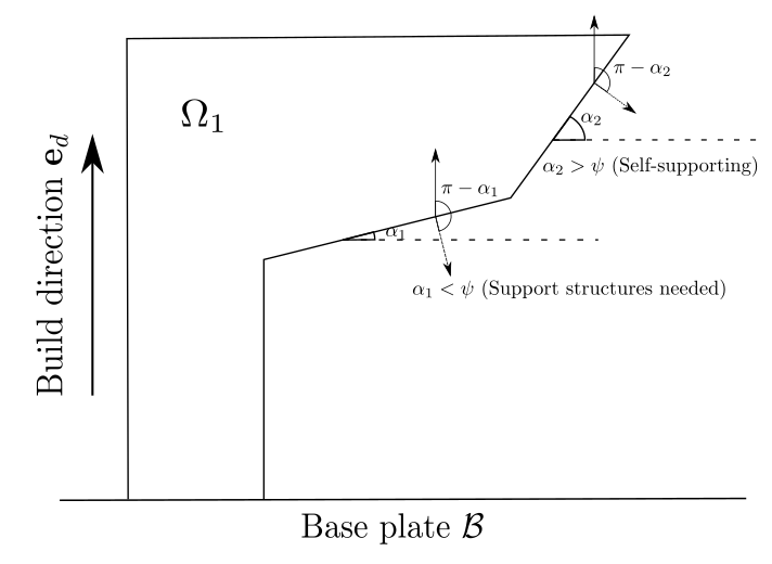
Then, there exists a critical threshold angle where the portion of is self-supporting (resp. requires support structures) if the overhang angle there is greater (resp. smaller) than . Conventional wisdom from practitioners puts the critical angle at [34, 60, 82] with the reasoning that every layer then has approximately 50% contact with the previous layer and thus it is well-supported from below, although there are some authors that propose smaller values for (e.g., in [61, 62]). Exact values of this critical angle also depend on the setting of the 3D printer as well as physical properties of the raw materials used. We mention that other works [67] consider an alternate definition, which is given as the angle from the vertical build direction to the outward unit normal of . Denoting this as , a simple calculation shows that . Then, regions where (typically if ) will require support structures.
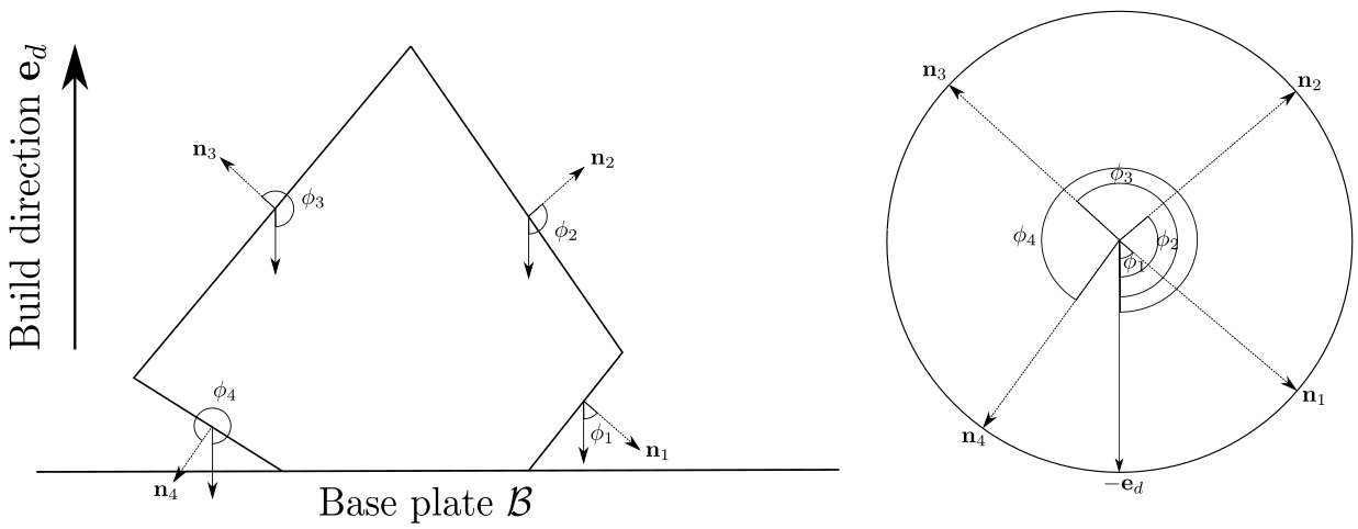
In this work we adopt the latter definition, but choose to define the overhang angle as the angle measured from the negative build direction to the outer unit normal, see Figure 2 and also [4, 30]. Then, given a critical angle threshold (expressed now in radians), the overhang angle constraint in the current context of shape and topology optimization would demand that an optimal geometry for the object has minimal regions where the overhang angles there do not lie in the interval (i.e., should be self-supporting as much as possible), in addition to other mechanical considerations such as minimal compliance.
For structural topology optimization we employ the phase field methodology proposed in [28], later popularized by many authors to other applications such as multi-material structural topology optimization [22, 89], compliance optimization [24, 78], topology optimization with local stress constraints [29], nonlinear elasticity [73], elastoplasticity [6], eigenfrequency maximization [45, 78], graded-material design [32], shape optimization in fluid flow [42, 43, 44], as well as resolution strategies for some inverse identification problems [21, 57]. The key idea is to cast the structural topology optimization problem as a constrained minimization problem for a phase field variable , where the geometry of an optimal design for the object can be realized as a certain level-set of . In the language of optimal control theory, acts as a control and influences a response function, e.g., the elastic displacement of the object, that is the solution to a system of partial differential equations (see (2.3) below). With an appropriate objective functional, for instance, a weighted sum of the mean compliance and a phase field formulation of the overhang constraint (see (2.7) below), we analyze the PDE-constrained minimization problem for an optimal design variable .
In the above references, previous authors employ an isotropic Ginzburg–Landau functional that has the effect of perimeter penalization (see Section 3 for more details), and in the current context this means no particular directions are preferred/discouraged in the optimization process. In this work we follow the ideas first proposed in [4, 34] that use an anisotropic perimeter functional as a geometric constraint for overhangs (see also similar ideas in [2] for support structures), and introduce a suitable anisotropic Ginzburg–Landau functional for the phase field optimization problem to enforce the overhang angle constraint. In one sense, our first novelty is that we generalize earlier works in phase field structural topology optimization by considering anisotropic energies. The precise formulation and details of the problem are given in the next sections. For more details regarding the use of anisotropy in phase field models we refer the reader to [15, 16, 46, 81].
Our second novelty is the analysis of the anisotropic phase field optimization problem. We establish the existence of minimizers (i.e., optimal designs) and derive first-order necessary optimality conditions. It turns out that our proposed approach to the overhang angle constraint requires an anisotropy function that is not continuously differentiable. In turn, the derivation of the associated necessary optimality conditions becomes non-standard. We overcome this difficulty with subdifferential calculus, and provide a characterization result for the subdifferential of convex functionals whose arguments are weak gradients. Then, we perform a formally matched asymptotic analysis for the optimization problem with a differentiable to infer the corresponding sharp interface limit.
Lastly, let us provide a non-exhaustive overview on related works that integrate the overhang angle constraint within a topology optimization procedure. Our closest counterpart is the work [4] which employs an anisotropic perimeter functional in a shape optimization framework implemented numerically with the level-set method. The authors observed that oscillations along the object boundary would develop even though the design complied with the angle constraint. This so-called dripping effect is attributed to instability effects of the anisotropic perimeter functional, brought about by the non-convexity of the anisotropy used in [4], see also Example 3.3 and Figure 10 below and the discussion in [52, Sec. 7.3]. An alternative mechanical constraint based on modeling the layer-by-layer construction process is then proposed to provide a different treatment of the overhangs and seems to suppress the dripping effect (see also [10] for similar ideas), but is computationally much more demanding. These boundary oscillations have also been observed earlier in [75], which used a Heaviside projection based integral to encode the overhang angle constraint within a density based topology optimization framework, and can be suppressed by means of an adaptive anisotropic filter introduced in [66]. Similar projection techniques for density filtering are used in [49], which was combined with an edge detection algorithm to evaluate feasible and non-feasible contours during optimization iterations. In [50], control of overhang angles is achieved by means of filtering with a wedge-shaped support, while in [92] an explicit quadratic function with respect to the design density is used to formulate the self-support constraint. A different approach was proposed in [58, 59] using a spatial filtering which checks element densities row-by-row and remove all elements not supported by the previous row. This idea is then extended in [60, 72, 83] to construct new filtering schemes that include other relevant manufacturing constraints. Another method was proposed in [51] using the frameworks of moving morphable components and moving morphable voids to provide a more explicit and geometric treatment of the problem, and is capable of simultaneously optimizing structural topology and build orientation. Finally, let us mention [85, 86], where a filter is developed based on front propagation in unstructured meshes that has a flexibility in enforcing arbitrary overhang angles. Focusing only on overhang angles in enclosed voids, [65] combined a nonlinear virtual temperature method for the identification of enclosed voids with a logarithmic-type function to constraint the area of overhang regions to zero.
The rest of this paper is organized as follows: in Section 2 we formulate the phase field structural optimization problem to be studied, and in Section 3 we describe our main idea of introducing anisotropy, along with some examples and relevant choices, as well as a useful characterization of the subdifferential of the anisotropic functional. The analysis of the structural optimization problem is carried out in Section 4, where we establish analytical results concerning minimizers and optimality conditions. The connection between our work and that of [4] is explored in Section 5 where we look into the sharp interface limit, and, finally, in Section 6 we present the numerical discretization and several simulations of our approach.
2 Problem formulation
In a bounded domain with Lipschitz boundary that exhibits a decomposition , we consider a linear elastic material that does not fully occupy . We describe the material location with the help of a phase field variable . In the phase field methodology, we use the level set to denote the region occupied by the elastic material, and to denote the complementary void region. These two regions are separated by a diffuse interface layer whose thickness is proportional to a small parameter . Since describes the material distribution within , complete knowledge of allows us to determine the shape and topology of the elastic material.
Notation.
For a Banach space , we denote its topological dual by and the corresponding duality pairing by . For any and , the standard Lebesgue and Sobolev spaces over are denoted by and with the corresponding norms and . In the special case , these become Hilbert spaces and we employ the notation with the corresponding norm . For convenience, the norm and inner product of are simply denoted by and , respectively. For our subsequent analysis, we introduce the space
Let us remark that, despite we employ bold symbols to denote vectors, matrices, and vector- or matrix-valued functions, we do not introduce a special notation to indicate the corresponding Lebesgue and Sobolev spaces. Thus, when those terms occur in the estimates, the corresponding norm is to be intended in its natural setting.
2.1 State system
To obtain a mathematical formulation that can be further analyzed, we employ the ersatz material approach, see [5], and model the complementary void region as a very soft elastic material. This allows us to consider a notion of elastic displacement on the entirety of , leading to the displacement vector and the associated linearized strain tensor
Let and be the fourth order elasticity tensors corresponding to the ersatz soft material and the linear elastic material, respectively, that satisfy the standard symmetric conditions
and assume there exist positive constants and such that for any non-zero symmetric matrices , :
where denotes the Frobenius inner product between two matrices. With the help of the phase field variable , we define an interpolation fourth order elasticity tensor as
where is a monotone function satisfying and . Then, it is clear that in the region (resp. ) we obtain the elasticity tensor (resp. ) by substituting (resp. ) into the definition of . As an example, we can consider
where is a constant and for any symmetric matrix ,
| (2.1) |
with identity matrix and Lamé constants and to obtain a linear interpolating elasticity tensor. Another example for uses a quadratic interpolation function
| (2.2) |
Let denote a body force and denote a surface traction force. On we assign a zero Dirichlet boundary condition for the displacement and on we assign a traction-free boundary condition. This leads to the following elasticity system for the displacement , representing the state system of the problem:
| (2.3a) | |||||
| (2.3b) | |||||
| (2.3c) | |||||
| (2.3d) | |||||
where denotes the outward unit normal to , and is defined as is a function introduced so that the body force only acts on the elastic material (where ) and not on the ersatz material (where ). We extend as if and as if .
The well-posedness of (2.3) is a simple consequence of [22, Thms. 3.1, 3.2], which we summarize as follows:
Lemma 2.1.
For any and , there exists a unique solution to (2.3) satisfying
| (2.4) |
where denotes the -dimensional Hausdorff measure. Moreover, there exists a positive constant , independent of , such that
| (2.5) |
In addition, let and with , and be the associated solution to (2.4). Then, there also exists a positive constant , depending on the data of the system and , but independent of the difference , such that
The above result provides a notion of a solution operator, also referred to as the control-to-state operator, where is the unique solution to (2.4) corresponding to . As such, we may view the phase field variable as a design variable that encodes the elastic response of the associated material distribution through the operator and seek an optimal material distribution that fulfills suitable constraints and minimizes some cost functional.
2.2 Cost functional and design space
We define the design space, i.e., the set of admissible design variables, as
| (2.6) |
where is a fixed constant for the mass constraint, and motivated by the context of additive manufacturing, we propose the following cost functional to be minimized:
| (2.7) |
In (2.7), the second term premultiplied by is the mean compliance functional, while the first term premultiplied by is an anisotropic Ginzburg–Landau functional with anisotropy function . We delay the detailed discussion on to the next section and remark here that for the isotropic case , , it is well-known that the Ginzburg–Landau functional is an approximation of the perimeter functional. Therefore, (2.7) can be viewed as a weighted sum between (anisotropic) perimeter penalization and mean compliance.
Lastly, for the non-negative potential function in (2.7), we require that it has as its global minima. While many choices are available, in light of the design space , we consider as the double obstacle potential
| (2.8) |
It is worth pointing out that it holds for . Then, the structural optimization problem we study can be expressed as the following:
| Minimize subject to and solving (2.3). | (P) |
3 Anisotropic Ginzburg–Landau functional
In the phase field methodology, the (isotropic) Ginzburg–Landau functional reads as
| (3.1) |
where and is a non-negative double-well potential that has as its minima, i.e., . Heuristically, the minimization of (3.1) in results in minimizers that take near constant values close to in large regions of the domain , which are separated by thin interfacial regions with thickness scaling with over which the functions transit smoothly from one value to the other. Formally in the limit these minimizers converge to functions that only take values in . This is made rigorous in the framework of -convergence by the seminal work of Modica and Mortola [68, 69].
To facilitate the forthcoming discussion, we review some basic properties for functions of bounded variations. For a more detailed introduction we refer the reader to [8, 36]. A function is a function of bounded variation in if its distributional gradient is a finite Radon measure. The space of all such functions is denoted as and its endowed with the norm , where for , its total variation is defined as
The space denotes the space of all functions taking values in . We say that a set is a set of finite perimeter, or a Caccioppoli set, if its characteristic function , where if and if , belongs to . The perimeter of a set of finite perimeter in is defined as
while its reduced boundary is the set of all points such that for all , with denoting the ball of radius centered at , and
The unit vector is called the measure theoretical unit inner normal to at , a theorem by De Giorgi yields the connection , see, e.g., [8]. Then, the result of Modica and Mortola [68, 69] can be expressed as follows: The -limit of the extended functional
is equal to
with the constant .
Remark 3.1.
For , setting leads to the relation , and hence
Of particular interest is the following property of -convergence, which states that if (i) is the -limit of , (ii) is a minimizer to for every , (iii) is a precompact sequence, then every limit of a subsequence of is a minimizer for . This provides a methodology to construct minimizers of as limits of minimizers to , provided the associated -limit is precisely .
Returning to our discussion and problem in additive manufacturing, in [4] it was proposed to use anisotropic perimeter functionals to model the overhang angle constraint. In our notation, for a set of bounded variation with as the measure theoretical inward unit normal, these functionals take the form
| (3.2) |
with a function . Two choices were suggested in [4]:
where is a fixed angle threshold, denotes the build direction, and , for , are given pattern functions with . The first choice penalizes the regions of the boundary where the angle between the outward normal and the negative build direction is smaller than , while the second choice compels the unit normal to be close to at least one of the directions .
A phase field approximation of the anisotropic perimeter functional (3.2) is the following anisotropic Ginzburg–Landau functional
| (3.3) |
where as before, is a double well potential with as its minima. Then, for a convex that is positively homogeneous of degree one (see (A1)), one has the analogue of the result by Modica and Mortola for anisotropic energies (see [19, 20, 27, 71], and also Lemma 5.1 below), that is
where the extended functionals and are defined as
| (3.4a) | ||||
| (3.4b) | ||||
This motivates our consideration of the objective functional (2.7) and of the study of the related minimization problem for the overhang angle constraint. Furthermore, let us formally state the corresponding sharp interface limit of the structural optimization problem as:
| Minimize subject to and solving (2.3), | () |
where and
Note that by Lemma 2.1, the solution operator is well-defined for . The connection between (P) and () will be explored in Section 5.
3.1 Anisotropy function, Wulff shape and Frank diagram
Consider an anisotropic density function satisfying
-
(A1)
is positively homogeneous of degree one:
which immediately implies .
-
(A2)
is positive for non-zero vectors:
-
(A3)
is convex:
Note that it is sufficient to assign values of on the unit sphere in , since by the one-homogeneity property (A1) we can define for any with
A consequence of the convexity assumption (A3) is that is continuous (in fact it is even locally Lipschitz continuous, see, e.g., [7, E4.6, p. 129]). Then, from (A2) we have that has a positive minimum on the compact set , and consequently by (A1), for . Thus, (A1)–(A3) yield the following property:
-
(A4)
is Lipschitz continuous and there exists a constant such that
Moreover, with in (A1) and in (A3), it is not difficult to verify that satisfies the triangle inequality. Hence, provided that for all , any satisfying (A1)–(A3) defines a norm on .
For such anisotropy density functions and smooth hypersurfaces with normal vector field , we define the anisotropic interfacial energy as
| (3.5) |
Then, the isoperimetric problem involves finding a hypersurface that minimizes under a volume constraint. This problem has been well-studied by many authors (see for instance [39, 40, 79, 80] and [52] and the references therein) and the solution is given as the boundary of the region called the Wulff shape [90]
| (3.6) |
where is the dual function of defined as
| (3.7) |
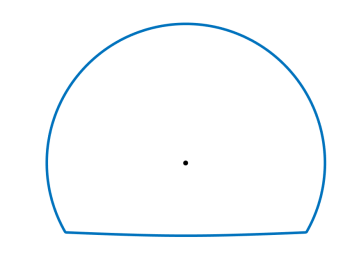
The dual function also satisfies (A1)–(A3) and hence we can view the Wulff shape as the 1-ball of . Besides the Wulff shape, another region of interest that is used to visualize the effects of the anisotropy is the Frank diagram [38], which is defined as the 1-ball of :
| (3.8) |
which, due to (A3), is always a convex subset of . To see how the shape of the boundary of determines which directions of unit sphere in is preferred by the anisotropic density function , let us consider three examples.
Example 3.1 (Isotropic case).
Consider for . Then, the associated Frank diagram is just the unit ball in , with boundary . As all points on the boundary are equidistant to the origin, all directions of the unit sphere in are equally preferable.
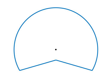
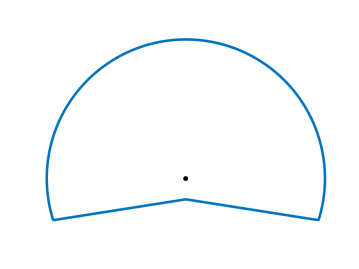
Example 3.2 (Convex example).
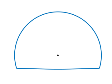
Consider the Frank diagram shown in the left of Figure 3, whose boundary is composed of a circular arc and a horizontal line . The black dot denotes the origin in . For any unit vector in , we denote by the angle it makes with the negative -axis measured anticlockwise (see also Figure 2). Then, there exists such that all unit vectors with angle in are associated with the horizontal line in Figure 3, while all unit vectors with angle in are associated with the circular arc . Notice, if the origin lies on , then , and is the upper semicircle.
Let and be arbitrary, and set , as their unit vectors. It is clear from the figure that , and since , by (A1) we see that
This implies that , and from the viewpoint of minimizing the interfacial energy in (3.5), directions are preferable to directions . Consequently, from the Frank diagram in Figure 3 we can see that the associated anisotropy density function prefers directions with angle in over directions with angle in .
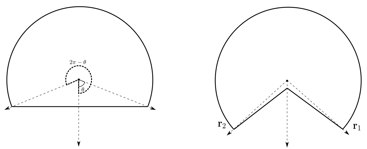
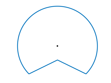
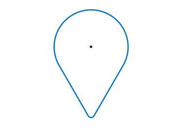
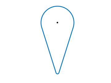
Example 3.3 (Non-convex example).
Consider the Frank diagram shown in the right of Figure 3, whose boundary encloses a non-convex set. Let and denote the two unit vectors whose angles, say and , respectively, associate to the two endpoints of the circular arc. From previous discussions, the anisotropy density function will prefer directions with angles in .
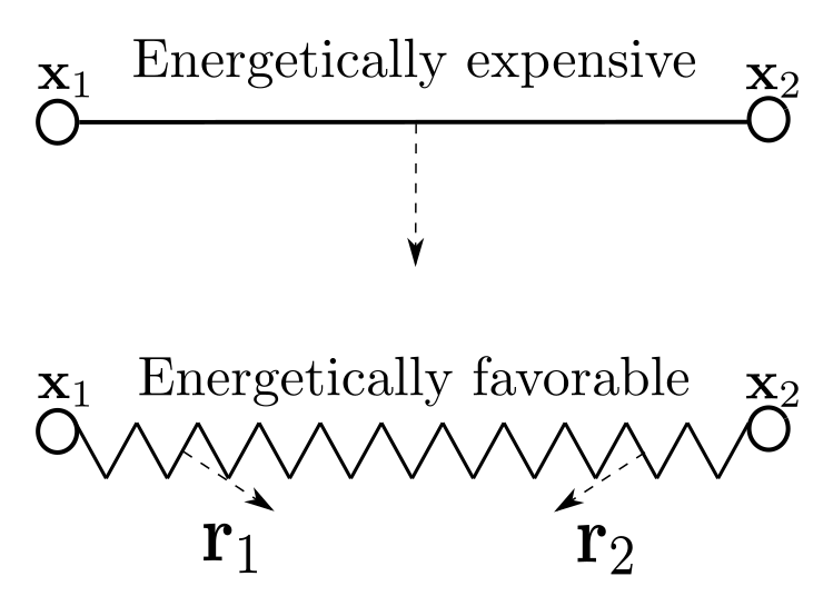
With such , consider two spatial points and at the same height, see Figure 4. Connecting them via a horizontal straight line is energetically expensive since this is associated to a direction with angle zero (where on the boundary of the Frank diagram is closest to the origin). An energetically more favorable connection is a zigzag path from and whose normal vectors oscillate between and . This is similar to a behavior termed “dripping effect” in [4] (see also [75, Fig. 15]), which is the tendency for shapes to develop oscillatory boundaries in order to meet the overhang angle constraints.
3.2 Relevant examples of anisotropic density function
Motivated by the above discussion, in this section we provide some examples of that achieve the Frank diagrams shown in Figure 3.
3.2.1 An example of a convex anisotropy
To fix the ideas, let us begin with the two-dimensional case. For a fixed constant , we consider the function
| (3.9) |
where the set will be determined in the following. To achieve the boundary of the Frank diagram shown in the left of Figure 3, we notice that is a circular arc of radius centered at the origin, while implies which is a horizontal line segment at height . Following the convention in Figure 2 where angles are measured anticlockwise from the negative -axis, we can parameterize the circular arc by for where , see Figure 3. Hence, the set in the definition (3.9) can be characterized as
Remark 3.2.
Note that in the limiting case , the above set is the entire plane . Hence we have the isotropic case for all , and is simply the unit circle.
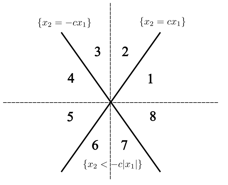
For a parametric characterization of the set , let and consider the two straight lines and dividing into eight regions (see Figure 5), which we label as Region in an anticlockwise direction starting from the positive -axis. Then, the horizontal straight line portion of the Frank diagram at height is contained in Regions 6 and 7, whose union is described by the set , while the circular arc portion is contained in Regions and , whose union is described by the set . Hence, a parameteric characterization of the set in (3.9) is
Generalizing to the -dimensional case, we obtain
| (3.10) |
From (3.10) we see that but it is not continuously differentiable at the points . Furthermore, it is clear that satisfies the assumptions (A1)–(A3) and hence (A4).
3.2.2 An example of a non-convex anisotropy
For completeness, we provide an example of an anisotropic function that yields a non-convex Frank diagram as seen in the right of Figure 3. Referring to the construction of the previous example, we present the two-dimensional case first. Fix and let denote the intersection of the two straight line segments (which we call and respectively) just below the origin. Denoting by the endpoint of the left line segment and by the endpoint of the right line segment that connects to the circular arc of radius , a short calculation shows that .
A choice of tangent vector for is so that a normal vector for is . Consider, for some constant to be identified,
for . This corresponds to Region 6 in the right of Figure 5 that contains the line segment , which can be parameterized as
Notice that satisfies (A1)–(A2) (due to the modulus), and a short calculation shows that for ,
Hence, choosing yields that for . Similarly, a choice of tangent vector for is , so that a normal vector for is . We consider
for which corresponds to Region 7 in Figure 5 that contains the line segment . Then, a short calculation shows that for . Thus, an example of an anisotropic function that give rise to a Frank diagram whose boundary is the right figure in Figure 3 is
| (3.11) |
for , and . Notice that in the limit , we recover the convex anisotropic function defined in (3.10).
To generalize to the -dimensional case, we notice that the lines and in the above discussion are now replaced by the lateral surface of a cone with apex , which can be parameterized as
Then, by similar arguments leading to (3.11), we obtain the function
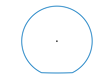
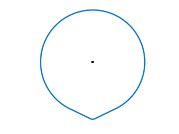
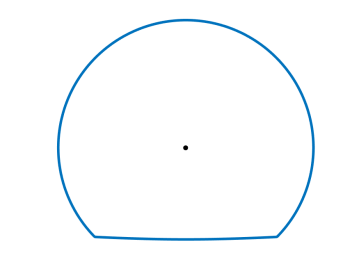
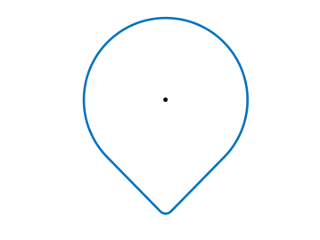
for , , where we can verify that for . In Figure 6 we display the Frank diagrams for non-convex anisotropy functions of the form (3.11) with and .
3.3 Subdifferential characterization
The analysis of the structural optimization problem (P) follows almost analogously as in [22]. The major difference is the anisotropic Ginzburg–Landau functional in (2.7). From the examples of discussed in the previous subsection, our interest lies in anisotropy density functions that are convex and continuous, but not necessarily , which necessitates a non-trivial modification to the analysis performed in [22]. In this subsection we focus only on the gradient part of (2.7) and investigate its subdifferential in preparation for the first-order necessary optimality conditions for (P) (cf. Theorem 4.2).
We define as
| (3.12) |
and from (A1)–(A4), it readily follows that is convex, continuous with , positive for non-zero vectors, positively homogeneous of degree two:
and there exist positive constants and such that
| (3.13) |
Associated to such a function , we consider the integral functional
| (3.14) |
Convexity of immediately imply that is convex, proper and weakly lower semicontinuous in , see, e.g., [35, Thm. 1, §8.2.2]. Consequently, its subdifferential , defined as
is a maximal monotone operator from to (see [13, Thm. 2.43]), which is equivalent to the property that, for any , there exists at least one solution with such that
Let us now provide a useful lemma that characterizes the subdifferential in terms of elements of (see also [13, p. 146, Problem 2.7]). Heuristically, elements of are the negative weak divergences of elements of .
Lemma 3.1.
Consider the map defined by
Then, for , it holds that
Remark 3.3.
If is smooth, convex, coercive with bounded second derivatives, i.e., there exists such that for all and , then the corresponding characterization of the subdifferential of can be found in [35, Thm. 4, §9.6.3]. Namely, is single-valued and .
Proof of Lemma 3.1.
To begin, fix , and let with for almost every satisfying for all . By the definition of the subgradient , we have
Choosing where is arbitrary, and integrating over we infer that
This shows and hence the inclusion .
For the converse inclusion, we show is a maximal monotone operator, and as is maximal monotone we obtain by definition for all . Thus, it suffices to study the solvability of the following problem: For , find a pair such that almost everywhere in and
| (3.15) |
This result can be obtained by following a strategy outlined in [12, Thm. 2.17]. First, from recalling the properties of in (3.13), we deduce that for ,
| (3.16) |
where the first inequality is obtained from applying the relation with the choice , and the second inequality is obtained from the second property of in (3.13) with the choice where is the canonical -th unit vector in . Taking the maximum over and then the supremum over all elements , the second inequality in (3.16) implies
| (3.17) |
Next, for , we introduce the Moreau–Yosida approximation of as
where denotes the identity map. The maximal monotonicity of guarantees that is a well-defined operator and it is bounded independently of (see [35, p. 524, Thms. 1 and 2]). It is well-known that is single-valued, Lipschitz continuous with Lipschitz constant , and is an element of . Then, by (3.16) and (3.17) (cf. [12, p. 84, (2.143)-(2.144)]), we infer from the identity that for all and , with constant from (3.13),
| (3.18a) | ||||
| (3.18b) | ||||
with constants independent of . We now consider the approximation problem: For , find such that
| (3.19) |
It is not difficult to verify that is monotone, demicontinuous (i.e., in implies in as ), and coercive (i.e., for some independent of ), and so by standard results (see, e.g., [12, p. 37, Cor. 2.3]) there exists at least one solution to in .
We then establish uniform estimates for whose weak limit in will be a solution to (3.15), thereby verifying the maximal monotonicity of and hence completing the proof. Choosing in (3.19) and recalling the identity , we obtain
| (3.20) | ||||
From (3.18) we immediately infer
which provides a uniform estimate for in with respect to . On the other hand, also from (3.18), particularly , we observe that
which implies, along a non-relabeled subsequence ,
| (3.21a) | |||||
| (3.21b) | |||||
| (3.21c) | |||||
for some limit functions and satisfying
To show that for almost every , for arbitrary and , we use the inequality
obtained from the relation and the monotonicity of . Then, passing to the limit with (3.21), as well as
we arrive at
Picking , so that , we see that the above reduces to
which implies and almost everywhere in . This shows that is a solution to (3.15) concluding the proof. ∎
4 Analysis of the structural optimization problem
By Lemma 2.1 the solution operator , where is the unique solution to (2.3) corresponding to the design variable , is well-defined. This allows us to consider the reduced functional ,
in the structural optimization problem (P). Invoking [35, Thm. 1, §8.2.2], the convexity of and hence of yields that the gradient term in (2.7) is weakly lower semicontinuous in . Then, following the proof of [22, Thm. 4.1] we obtain the existence of an optimal design to (P).
Proof.
Since the proof is now rather standard, we only sketch some of the essential details. Using the bound (2.5) we infer that the reduced functional is bounded from below in . This allows us to consider a minimizing sequence such that as . Then, again by (2.5) and also (A4) we deduce that is uniformly bounded in , from which we extract a non-relabeled subsequence converging weakly to in . As is a convex and closed set, hence weakly sequentially closed, we infer also and by passing to the limit infimum of , employing the weak lower semicontinuity of the gradient term in (2.7) and also the weak convergence in we infer that , which implies that is a solution to (P). ∎
To derive the first-order optimality conditions, we first take note of the following result concerning the Fréchet differentiability of the solution operator , which can be inferred from [22, Thm. 3.3]:
Lemma 4.1.
Let and . Then is Fréchet differentiable at as a mapping from to . Moreover, for every , and
where is the unique solution to the linearized system
| (4.1) |
for all with .
Then, we introduce the adjoint system for the adjoint variable associated to , whose structure is similar to the state equation (2.3) for :
| (4.2a) | |||||
| (4.2b) | |||||
| (4.2c) | |||||
| (4.2d) | |||||
Via a similar argument (see also [22, Thm. 4.3]), the well-posedness of the adjoint system is straightforward:
Lemma 4.2.
Our main result is the following first-order optimality conditions for the structural optimization problem with anisotropy (P):
Theorem 4.2.
Proof.
Recalling the definition of the functional in (3.14), we introduce
| (4.5) |
so that the reduced functional can be expressed as . Using the differentiability of we infer that is also Fréchet differentiable with derivative at in direction given as
| (4.6) |
where is unique solution to the linearized system (4.1) and . We can simplify this using the adjoint system by testing (4.3) with and testing (4.1) with to obtain the identity
so that, together with the relation , (4.6) becomes
| (4.7) |
On the other hand, the convexity of and the optimality of imply that
holds for all and arbitrary . Dividing by and passing to the limit yields
| (4.8) |
The above inequality allows us to interpret as a solution to the convex minimization problem
| (4.9) |
denotes the indicator function of the set . Using the well-known sum rule for subdifferentials of convex functions, see, e.g., [13, Cor. 2.63], the inequality (4.8) can be interpreted as
where denotes the subdifferential mapping in . This implies the existence of elements and such that
| (4.10) |
For arbitrary , by definition of we have
Then, using Lemma 3.1, there exists with almost everywhere in and
The optimality condition (4.4) is then a consequence of the above and (4.7) with . ∎
Remark 4.1.
An alternate formulation of the optimality condition (4.4) is as follows: There exist , , and a Lagrange multiplier for the mass constraint such that
| (4.11) | ||||
for all . In the above, the subdifferential of the indicator function has the explicit characterization
Indeed, instead of (4.9) we can interpret as a solution to the minimization problem
which then yields the existence of elements and such that
For arbitrary , we test the above equality with , where , and on noting that
this yields (4.11) with Lagrange multiplier .
5 Sharp interface asymptotics
Our interest is to study the behavior of solutions under the sharp interface limit , which connects our phase field approach with the shape optimization approach of [4].
5.1 -convergence of the anisotropic Ginzburg–Landau functional
We begin with the -convergence of the extended anisotropic Ginzburg–Landau functional (3.4a) to the extended anisotropic perimeter functional (3.4b), which is formulated as follows:
Lemma 5.1.
Let be an open bounded domain with Lipschitz boundary. Let satisfy (A1)–(A3), is a double well potential with minima at and define . Then, for any
-
If is a sequence such that and strongly in , then with .
-
Let . Then, there exists a sequence of Lipschitz continuous functions on such that a.e. in , strongly in , for all , and .
-
Let be a sequence satisfying . Then, there exists a non-relabeled subsequence and a limit function such that strongly in with .
The first and second assertions are known as the liminf and limsup inequalities, respectively, while the third assertion is the compactness property. In the following, we outline how to adapt the proofs of [20, Thms. 3.1 and 3.4] for the -convergence result in the multi-phase case. Our present setting corresponds to the case in their notation.
Proof.
For arbitrary , we introduce the associated vector where and . Then, take values in the Gibbs simplex . Setting and , we consider a multiple-well potential satisfying and
| (5.1) |
where the latter relation connects to defined in (2.8). Denoting by the set of 2-by- matrices, we consider a function defined as , where satisfies (A1)–(A3), and denotes the -th row of . Taking for yields that and
| (5.2) |
by the relation and the one-homogeneity of . Assumptions (A1)–(A3) on ensures the function defined above fulfills the corresponding assumptions in [20, p. 80], and thus by [20, Thm. 3.1], the extended functional
-converges in to a limit functional
where the definitions of the set , normal and function can be found in [20, p. 78, p. 81]. It is clear that for , and our aim is to show for . For a fixed vector , let denote the -dimensional cube of side lying in the orthogonal complement centered at the origin. Following [20], a function is -periodic if for every and every , with as directions of the sides of . Setting we denote by the class of all functions which are -periodic and satisfy and . Then, by [20, (6)], the integrand in the -limit functional has the representation formula
where . To simplify the above expression, for a fixed , consider a function of the form for a monotone function such that and satisfies . For the choice we have the explicit solution (known also as the optimal profile)
| (5.3) |
Furthermore, multiplying the equality by and integrating yields the so-called equipartition of energy for all . Then, it is clear that . By (A1), (5.1) and (5.2), as well as Fubini’s theorem, for we have , and
after a change of variables and using the equipartition of energy . Hence, we obtain the identification with constant . Then, for , we define via the relation , and this allows us to identify and consequently . Then, the liminf, limsup and compactness properties follow directly from [20, Thms. 3.1 and 3.4]. ∎
5.2 Formally matched asymptotic analysis
In this section we consider an anisotropy function satisfying (A1)–(A3) in the structural optimization problem (P), as well as a more regular body force . The differentiability of implies the characterization of the subdifferential as the singleton set , where
Then, the corresponding optimality condition for a minimizer to (P) becomes
| (5.4) | ||||
and its strong formulation reads as (see (4.11))
| (5.5a) | ||||
| (5.5b) | ||||
with Lagrange multiplier for the mass constraint. Our aim is to perform a formally matched asymptotic analysis as , similar as in [25, Sec. 5], in order to infer the sharp interface limit of (5.5). The method proceeds as follows, see [31]: formally we assume that the domain admits a decomposition , where is an annular domain and satisfies
| (5.6) |
The zero level set is assumed to converge to a smooth hypersurface as , and that admit an outer expansion in regions in as well as an inner expansion in regions in . We substitute these expansions (in powers of ) in (2.3) and (5.5), collecting terms of the same order of , and with the help of suitable matching conditions connecting these two expansions, we deduce an equation posed on . For an introduction and more detailed discussion of this methodology we refer to [37, 47].
To start, let us collect some useful relations. As is positively homogeneous of degree one, taking the relation for and and differentiating with respect to , and also with respect to leads to
| (5.7) |
with the latter relation showing that is positively homogeneous of degree zero. Then, it is easy to see is positively homogeneous of degree one. Next, from (3.12), we see that is positively homogeneous of degree two. Taking the relation and differentiating with respect to twice leads to
| (5.8) |
where with denoting the Hessian matrix of . Lastly, differentiating the relation with respect to and setting yields
| (5.9) |
5.2.1 Outer expansions
For points in , we assume an outer expansion of the form
where all functions are sufficiently smooth and the summations converge. From (5.6) we deduce that
Setting and , it holds that . Then, substituting the outer expansion into (2.3), we obtain to order the following system of equations
| (5.10a) | |||||
| (5.10b) | |||||
| (5.10c) | |||||
| (5.10d) | |||||
Moreover, from the definition of the Lagrange multiplier we see that
| (5.11) | ||||
It remains to derive the boundary conditions for (5.10) holding on , which can be achieved with the inner expansions.
5.2.2 Inner expansions
We assume the outer boundary and inner boundary of the annular region can be parameterized over the smooth hypersurface . Let denote the unit normal of pointing from to , and we choose a spatial parameter domain with a local parameterization of . Let denote the signed distance function of with if , and denote by the rescaled signed distance. Then, by the smoothness of , there exists such that for all , we have the representation
where . In particular, is the projection of to along the normal direction. This representation allows us to infer the following expansion for gradients and divergences [47]:
| (5.12) |
for scalar functions and vector functions . In the above is the surface gradient on and is the surface divergence. Analogously, for a vector function , we find that
For points close by in , we assume an expansion of the form
5.2.3 Matching conditions
In a tubular neighborhood of , we assume the outer expansions and the inner expansions hold simultaneously. Since are assumed to be graphs over , we introduce the functions such that . Furthermore, we assume an expansion of the form
is valid. As converge to , in the computations below we will deduce the values for . Then, by comparing these two expansions in this intermediate region we infer matching conditions relating the outer expansions to the inner expansions via boundary conditions for the outer expansions. For a scalar function admitting an outer expansion and an inner expansion , it holds that (see [31] and [47, Appendix D])
for . Consequently, we denote the jump of a quantity across as
5.2.4 Analysis of the inner expansions
We introduce the notation for a second order tensor . Plugging in the inner expansions to the state equation (2.3), to leading order we find that
Taking the product with and by the symmetry of we have the relation
Integrating over and by parts, using and by the matching condition leads to
Coercivity of yields that and hence . This implies is constant in and by the matching conditions we obtain
| (5.13) |
Then, using , to the next order we obtain from the state equation (2.3)
| (5.14) |
Integrating over and using the matching condition
we obtain
| (5.15) |
From the optimality condition (5.5a), to leading order we obtain the trivial equality due to . Recalling (5.11) for , to the next order of (5.5a) we have
| (5.16) |
where we again use to see that no terms from the elastic part contribute at order , the expression (5.12) for the divergence in the inner variables, the relation from (5.7), the fact that is positively homogeneous of degree one, so that
as well as the fact that is independent of . We now construct a solution to (5.16) fulfilling the conditions as as per the matching conditions, and also satisfies . Let be the monotone function defined in (5.3) which satisfies the boundary value problem
with and for all . We define , and a short calculation shows that
The property and the matching conditions for provide the identifications
Moreover, since is monotone and is positive, we can infer that . Now, multiplying (5.16) with and integrating over yields the so-called equipartition of energy
after using and . Performing another integration over leads to the relation
| (5.17) |
To the next order , we find that
| (5.18) | ||||
The aim is to multiply the above with and integrate over , but first, let us derive some useful relations. Using the symmetry of the elasticity tensor and , we deduce that, with the shorthand ,
Hence, together with from (5.14) and the matching conditions we obtain the relation
By (5.8), (5.9), (5.16), (5.17) and the matching conditions of , we have
Hence,
and upon multiplying (5.18) with and integrate over , employ the matching conditions leads to the following solvability condition for :
| (5.19) | ||||
Note that the assumed higher regularity allows us to define on . Thus, the sharp interface limit consists of the system (5.10) posed in , along with the boundary conditions (5.13), (5.15) and (5.19) on .
Remark 5.1 (Isotropic case).
In the isotropic case , for unit normals of , we have that and , where is the mean curvature of . Then, choosing so that , we observe that (5.19) simplifies to
which coincides with the formula obtained from [23, (24)] with adjoint , zero eigenstrain , Lagrange multiplier for the mass constraint, and that satisfies thanks to (5.13).
5.3 Relation to shape derivatives derived in [4]
To relate our work with the setting of [4], we first set in (5.10), and neglect all the equations posed in . Then, the state equation [4, (2.1)] can be obtained by writing as , as in (5.10). Note that in this setting the free boundary is identified with the traction-free part of . Furthermore, the normal vector in [4] on is equal to in our notation.
Writing as , the anisotropic perimeter functional defined in [4, (3.1)] can be expressed as in (3.2), and in terms of our notation its shape derivative is given as (compare [4, Prop. 3.1])
for admissible vector fields of sufficient smoothness, where we used that is positively homogeneous of degree zero (cf. (5.7)) and the identity . Here we point out a typo in the manuscript, where written there should in fact be (compare [34, Prop. 8]).
Now, consider the shape optimization problem of minimizing with the mean compliance
Then, with sufficiently smooth solutions, its shape derivative in our notation is (see [4, p. 299])
where in the above we have applied the integration by parts formula
as well as the relation from (5.7) to cancel the terms involving . Hence, the strong formulation of is
This coincides with the identity obtained if we neglect the Lagrange multiplier, set and in (5.19), and also use the relation from (5.15).
6 Numerical approximation
6.1 BGN anisotropies
For the numerical approximation of an optimal design variable to the structural optimization problem (P), we first consider a discretization of the variational inequality (5.4) with differentiable . In general, the term is highly nonlinear, and to facilitate the subsequent discussion regarding its discretization we first consider a matrix-type reformulation of the anisotropy density function introduced by the works of the first and third authors, see, e.g., [14, 15, 16] for more details.
Suppose for some , the anisotropy density function can be expressed as
| (6.1) |
with symmetric positive definite matrices for . Then, a short calculation shows that
and recalling that , we infer also
For close to , we now perform a linearization , where
so that
Furthermore, as are symmetric positive definite, the matrix is also symmetric positive definite for all . We term anisotropies that are of the form (6.1) as BGN anisotropies. Notice that for the definition of the linearized matrix it is sufficient to have anisotropy densities . However, due to our examples (3.10) and (3.11) it will turn out that the corresponding are no longer constant matrices. Thus, inspired by the works [14, 15, 16] we extend their approach to the case where are piecewise constant and dependent on , as shown in the following examples. In our numerical approximation to the optimality condition detailed in the next section we simply replace by , where now involves piecewise constant matrices .
Example 6.1.
The convex anisotropy (3.10) can be expressed as an extended BGN anisotropy
where for ,
In turn, this provides us with the linearization matrix .
Example 6.2.
The nonconvex anisotropy (3.11) can be written as an extended BGN anisotropy
where for ,
Then, the linearized matrix is given by .
For numerical simulations we also consider regularizations of the convex anisotropy in (3.10) of the form
| (6.2) |
for . This can also be expressed as an extended BGN anisotropy with , where we take , ,
The linearization matrix has the form
In Figure 7 we visualize the Frank diagram and Wulff shape of the anisotropy (6.2) in two spatial dimensions with and , , , .
6.2 Finite element discretization
Let be a regular triangulation of into disjoint open simplices. Associated with are the piecewise linear finite element spaces
where we denote by the set of all affine linear functions on . In addition we define the convex subsets
| (6.3) |
where denotes the –inner product on , as well as
| (6.4) |
We now introduce a finite element approximation of the structural optimization problem (P) and the optimality conditions described above. Given , find such that
| (6.5a) | |||
| (6.5b) | |||
Here denotes the time step size, is the usual mass lumped –inner product on , and for any fourth order tensor and any matrices and . We implemented the scheme (6.5) with the help of the finite element toolbox ALBERTA, see [77]. To increase computational efficiency, we employ adaptive meshes, which have a finer mesh size within the diffuse interfacial regions and a coarser mesh size away from them, see [11, 18] for a more detailed description. Clearly, the system (6.5a) decouples, and so we first solve the linear system (6.5a) in order to obtain , and then solve the variational inequality (6.5b) for . We employ the package LDL, see [33], together with the sparse matrix ordering AMD, see [9], in order to solve (6.5a). For the variational inequality (6.5b) we employ a secant method as described in [26] to satisfy the mass constraint , and use a nonlinear multigrid method similar to [55] for solving the variational inequalities over that arise as the inner problems for the secant iterations. The second method always converged in at most five steps. Finally, to increase the efficiency of the numerical computations in this paper, at times we exploit the symmetry of the problem and perform the computations in question only on half of the desired domain . In those cases we prescribe “free-slip” boundary conditions for the displacement field on the symmetry plane , that is, we replace (6.4) with
| (6.6) |
All computations performed in this work are for spatial dimension . For the remainder of the paper we consider the quadratic interpolation function (2.2) in the elasticity tensor , forcing , objective functional weightings and unless further specified.
6.3 Numerical simulations
6.3.1 Optimality condition without elasticity
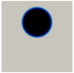
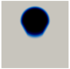
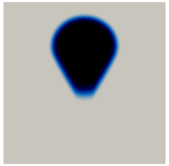
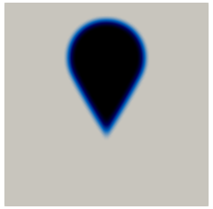
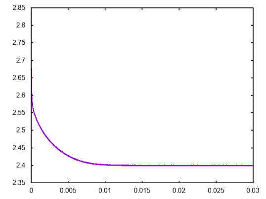
We first investigate the setting with , so that (6.5a) yields and (6.5b) reduces to an Allen–Cahn variational inequality on . From the discussion in Section 3, this is a phase field approximation of the volume preserving anisotropic mean curvature flow (due to the mass constraint), and it is expected that the long time behavior of solutions to display the Wulff shape (3.6) corresponding to the anisotropy , see Figure 7. In Figure 8 we display snapshots of the solution at times , , and with anisotropy (6.2) for parameter values , and . We notice from the bottom plot of the discrete Ginzburg–Landau energy that it is decreasing over time, and on the top right we observe the expected Wulff shape attained near equilibrium.
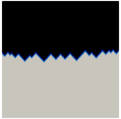
6.3.2 Dripping effect of a straight interface
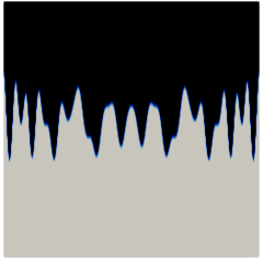
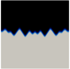
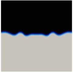
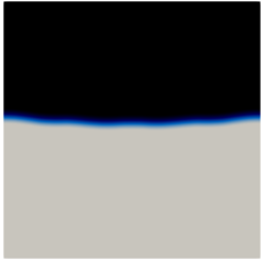
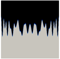
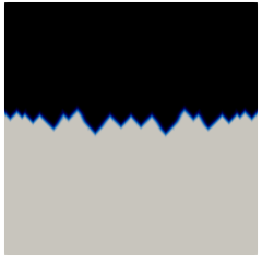
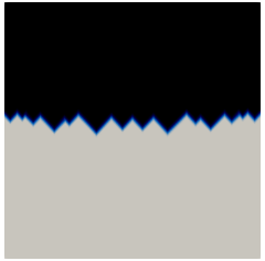
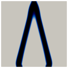
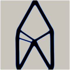
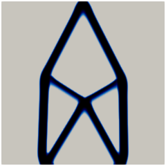
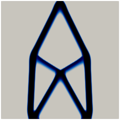
Next, we investigate the role of the convexity/non-convexity of in the generation of the dripping effect [4, 10, 75]. We solve (6.5) with and initial condition taken as some large perturbation of a straight interface. Taking (6.2) as the anisotropy with , and , in Figure 9 we display the snapshots of the solution at times , , and , where it is clear that the oscillations are dampened over time. Thus, with a convex anisotropy the dripping effect is suppressed. In contrast, taking as the non-convex anisotropy (3.11) with now yields Figure 10, where the corresponding snapshots of the solution at times , , , are displayed. Here we clearly observe the behavior described in Example 3.3.
6.3.3 Cantilever beam computation
Inspired by [4, Figure 8], for the state system (2.3), we consider the setting
| (6.7) | ||||
with and a positive constant. Note that the domain we use here is larger than the setting in [4]. This is done to to avoid the influence of the domain boundary on the growth of the interfacial layer . As in [4] we consider an elastic material with a normalized Young’s modulus and a Poisson ratio . The corresponding Lamé constants in the elasticity tensor (2.1) can be calculated through the well-known relations
| (6.8) |
For and , we solve the full optimality condition (6.5) with the convex regularized anisotropy (6.2) and compare the steady states for and a range of . Note that smaller values of indicate a stronger anisotropy. The results are displayed in Figure 11, where we taken random initial data with mass . Note that corresponds to the isotropic case, see Remark 3.2, and as decreases, we observe the interior connecting bridges in the cantilever beam become steeper in slope, up until where a design without interior structure is favored.
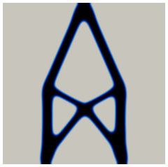
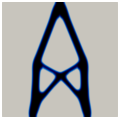
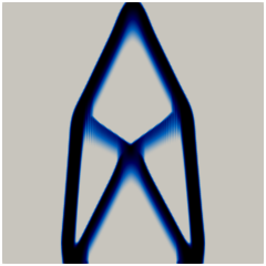
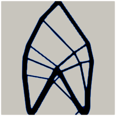
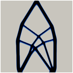
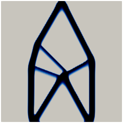
In Figure 12 we provide a more detailed comparison of the cantilever beam designs for the isotropic case and the strongly anisotropic cases with loading magnitudes and . In both situations, the anisotropic designs exhibit less interior structures and connecting bridges with steeper slopes than the isotropic designs, which is to be expected from the construction of . It is worth mentioning that some (but not all) of the interfacial regions (colored deep blue) are thicker for smaller values of . This is attributed to the fact that, from the expression of obtained in the formally matched asymptotic analysis in Section 5.2, the interfacial thickness at a spatial point in the transformed coordinate system is proportional to with unit normal . Recalling the left of Figure 3, the normal vectors with directions associated to the line segment attain higher values of , and thus a thicker interfacial region, compared to directions associated with the circular arc . Smaller values of amplify the thickness as the line segment is closer to the origin, leading to higher values of .
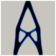
In Figure 13 we display refined designs taking as initial conditions the final states in Figure 12 as well as a smaller value of . The overall designs are similar to Figure 12 with some minor changes, particularly for the isotropic case with . We also note that the thicknesses of the interfacial layers in Figure 13 are smaller than those in Figure 12, particularly for , which is due to the smaller values of used.
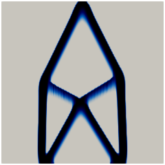
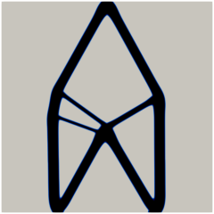
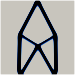
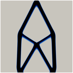
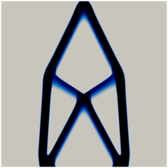
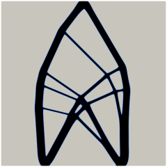
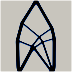
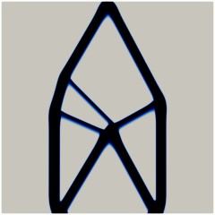
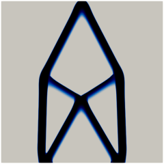
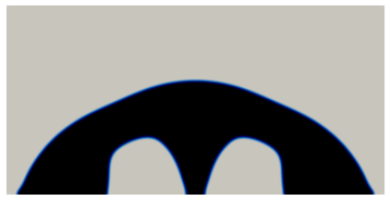
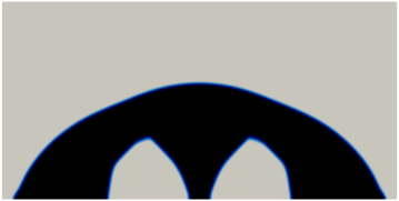
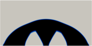
6.3.4 Bridge construction
Our last numerical simulation is inspired by [89, Figure 4], where we use the half-domain setup
For an elastic material with and , we investigate the optimal designs with the convex regularized anisotropy (6.2). In Figure 14 we display results for , , starting from random initial data with mass . Although the overall shapes are rather similar in all three cases, we observe the anisotropic cases (middle and right figures) have sharper corners on the underside of the bridge, whereas the underside of the isotropic case (left figure) is smoother.
Acknowledgments
The work of KFL is supported by the Research Grants Council of the Hong Kong Special Administrative Region, China [Project No.: HKBU 14302218].
References
- [1] O. Abdulhammed, A. Al-Ahmari, W. Ameen and S.H. Mian. Additive manufacturing: Challenges, trends, and applications. Adv. Mech. Engrg. 11 (2019), 1–27
- [2] G. Allaire, M. Bihr and B. Bogosel. Support optimization in additive manufacturing for geometric and thermo-mechanical constraints. Struct. Multidiscip. Optim. 61 (2020) 2377–2399
- [3] G. Allaire and B. Bogosel. Optimizing supports for additive manufacturing. Struct. Multidiscip. Optim. 58 (2018) 2493–2515
- [4] G. Allaire, C. Dapogny, R. Estevez, A. Faure and G. Michailidis. Structural optimization under overhang constraints imposed by additive manufacturing technologies. J. Comput. Phys. 351 (2017) 295–328
- [5] G. Allaire, F. Jouve and A.-M. Toader. Structural optimization using sensitivity analysis and a level-set method. J. Comput. Phys. 194 (2004) 363–393
- [6] S. Almi and U. Stefanelli. Topology optimization for incremental elastoplasticity: A phase-field approach. SIAM J. Control Optim. 59 (2021) 339–364
- [7] H.W. Alt. Linear Functional Analysis: An Application-Oriented Introduction. Springer-Verlag London, 2016
- [8] L. Ambrosio, N. Fusco and D. Pallara. Functions of Bounded Variation and Free Discontinuity Problems. Oxford mathematical monographs. Clarendon Press, 2000
- [9] P.R. Amestoy, T.A. Davis and I.S. Duff. Algorithm 837: AMD, an approximate minimum degree ordering algorithm. ACM Trans. Math. Software 30 (2004) 381–388
- [10] O. Amir and Y. Mass. Topology optimization for staged construction. Struct. Multidiscip. Optim. 57 (2017) 1679–1694
- [11] L. Baňas and R. Nürnberg. Finite element approximation of a three dimensional phase field model for void electromigration. J. Sci. Comp. 37 (2008) 202–232
- [12] V. Barbu. Nonlinear Differential Equations of Monotone Types in Banach Spaces. Springer Science & Business Media, 2010
- [13] V. Barbu and T. Precupanu. Convexity and Optimization in Banach Spaces. Springer Netherlands, 2012; 4th edition
- [14] J.W. Barrett, H. Garcke and R. Nürnberg. Numerical approximation of anisotropic geometric evolution equations in the plane. IMA J. Numer. Anal. 28 (2008) 292–330
- [15] J.W. Barrett, H. Garcke and R. Nürnberg. On the stable discretization of strongly anisotropic phase field models with applications to crystal growth. ZAMM Z. Angew. Math. Mech. 93 (2013) 719–732
- [16] J.W. Barrett, H. Garcke and R. Nürnberg. Stable phase field approximations of anisotropic solidification. IMA J. Numer. Anal. 34 (2014) 1289–1327
- [17] J.W. Barrett, H. Garcke and R. Nürnberg. Parametric finite element approximations of curvature driven interface evolutions. Handb. Numer. Anal. 21 (2020) 275–423
- [18] J.W. Barrett, R. Nürnberg and V. Styles. Finite element approximation of a phase field model for void electromigration. SIAM J. Numer. Anal. 42 (2004) 738–772
- [19] A.C. Barroso and I. Fonseca. Anisotropic singular perturbations - the vectorial case. Proc. Roy. Soc. Edinburgh Sect. A 124 (1994) 527–571
- [20] G. Bellettini, A. Braides and G. Riey. Variational approximation of anisotropic functionals on partitions. Annali di Matematica 184 (2005) 75–93
- [21] E. Beretta, L. Ratti and M. Verani. Detection of conductivity inclusions in a semilinear elliptic problem arising from cardiac electrophysiology. Commun. Math. Sci. 16 (2018) 1975–2002
- [22] L. Blank, H. Garcke, M. Hassan Farshbaf-Shaker and V. Styles. Relating phase field and sharp interface approaches to structural topology optimization. ESAIM: Control Optim. Calc. Var. 20 (2014) 1025–1058
- [23] L. Blank, H. Garcke, C. Hecht and C. Rupprecht. Sharp interface limit for a phase field model in structural optimization. SIAM J. Control Optim. 54 (2016) 1558–1584
- [24] L. Blank, H. Garcke, L. Sarbu, T. Srisupattarawanit, V. Styles and A. Voigt. Phase-field approaches to structural topology optimization, in Constrained optimization and optimal control for partial differential equations, vol. 160 of Internat. Ser. Numer. Math., Birkhäuser/Springer Basel AG, Basel, 2012, 245–256
- [25] L. Blank, H. Garcke, L. Sarbu and V. Styles. Primal-dual active set methods for Allen–Cahn variational inequalities with non-local constraints. Numer. Methods Partial Differential Equations 29 (2013) 999–1030
- [26] J.F. Blowey and C.M. Elliott. Curvature dependent phase boundary motion and parabolic double obstacle problems, in Degenerate diffusions (Minneapolis, MN, 1991), vol. 47 of IMA Vol. Math. Appl., Springer, New York, 1993, 19–60
- [27] G. Bouchitté. Singular Perturbations of Variational Problems Arising from a Two-Phase Transition Model. Appl. Math. Optim. 21 (1990) 289–314
- [28] B. Bourdin and A. Chambolle. Design-dependent loads in topology optimization. ESAIM: Control Optim. Cal. Var. 9 (2003) 19–48
- [29] M. Burger and R. Stainko. Phase-field relaxation of topology optimization with local stress constraints. SIAM J. Control Optim. 45 (2006) 1447–1466
- [30] S. Cacace, E. Cristiani and L. Rocchi. A Level Set Based Method for Fixing Overhangs in 3D Printing. Appl. Math. Model. 44 (2017) 446–455
- [31] J. Cahn, C.M. Elliott and A. Novick-Cohen. The Cahn–Hilliard equation with a concentration dependent mobility: motion by minus the Laplacian of the mean curvature. Euro. J. Appl. Math. 7 (1996) 287–301
- [32] M. Carraturo, E. Rocca, E. Bonetti, D. Hömberg, A. Reali and F. Auricchio. Graded-material design based phase-field and topology optimization. Comput. Mech. 64 (2019) 1589–1600
- [33] T.A. Davis, Algorithm 849: a concise sparse Cholesky factorization package. ACM Trans. Math. Software 31 (2005) 587–591
- [34] C. Dapogny, A. Faure, G. Michailidis, G. Allaire, A. Couvelas and R. Estevez. Geometric constraints for shape and topology optimization in architectural design. Comput. Mech. 59 (2017) 933–965
- [35] L.C. Evans. Partial Differential Equations. Vol. 19 of Graduate Studies in Mathematics, AMS, 2010
- [36] L.C. Evans and R. Gariepy. Measure Theory and Fine Properties of Functions. Math. Chem. Ser. CRC Press, Boca Raton, FL. 1992
- [37] P.C. Fife and O. Penrose. Interfacial dynamics for thermodynamically consistent phase-field models with nonconserved order parameter. J. Differential Equations 16 (1995) 1–49
- [38] F.C. Frank. The geometrical thermodynamics of surfaces. Am. Soc. Metals (1963) 1–15
- [39] I. Fonseca. The Wulff Theorem revisited. Proc. Roy. Soc. London 432 (1991) 125–145
- [40] I. Fonseca and S. Müller. A uniqueness proof for the Wulff Theorem. Proc. Roy. Soc. Edinburgh: Sec. A Math. 119 (1991) 125–136
- [41] H. Garcke, The -limit of the Ginzburg–Landau energy in an elastic medium. AMSA 18 (2008) 345–379
- [42] H. Garcke and C. Hecht. Apply a phase field approach for shape optimization of a stationary Navier-Stokes flow. ESAIM: Control Optim. Cal. Var. 22 (2016) 309–337
- [43] H. Garcke and C. Hecht. Shape and topology optimization in Stokes flow with a phase field approach. Appl. Math. Optim. 73 (2016) 23–70
- [44] H. Garcke, C. Hecht, M. Hinze, C. Kahle and K.F. Lam. Shape optimization for surface functionals in Navier–Stokes flow using a phase field approach. Interfaces Free Bound. 18 (2016) 219–261
- [45] H. Garcke, P. Hüttl and P. Knopf. Shape and topology optimization involving the eigenvalues of an elastic structure: A multi-phase-field approach. Adv. Nonlinear Anal. 11 (2022) 159–197
- [46] H. Garcke, B. Nestler and B. Stoth. On anisotropic order parameter models for multi0phase systems and their sharp interface limits. Phys. D 115 (1998) 87–108
- [47] H. Garcke and B. Stinner. Second order phase field asymptotics for multi-component systems. Interfaces Free Bound. 8 (2006) 131–157
- [48] N. Gardan and A. Schneider. Topological optimization of internal patterns and support in additive manufacturing. J. Manuf. Syst. 37 (2014) 417–425
- [49] A. Garaigordobil, R. Ansola, J. Santamaría and I. Fernández de Bustos. A new overhang constraint for topology optimization of self-supporting structures in additive manufacturing. Struct. Multidiscip. Optim. 58 (2018) 2003–2017
- [50] A.T. Gaynor and J.K. Guest. Topology optimization considering overhang constraints: Eliminating sacrificial support material in additive manufacturing through design. Struct. Multidiscip. Optim. 54 (2016) 1157–1172
- [51] X. Guo, J. Zhou, W. Zhang, Z. Du, C. Liu and Y. Liu. Self-supporting structure design in additive manufacturing through explicit topology optimization. Comput. Methods Appl. Mech. Engrg. 323 (2017) 27–63
- [52] M.E. Gurtin. Thermomechanics of evolving phase boundaries in the plane. Oxford University Press, 1993
- [53] A. Hussein, L. Hao, C. Yan, R. Everson and P. Young. Advanced lattice support structures for metal additive manufacturing. J. Mater. Process. Technol. 213 (2013) 1019–1026
- [54] J. Jiang, X. Xu and J. Stringer. Support Structures for Additive Manufacturing: A Review. J. Manuf. Mater. Process. 2 (2008) 64 (23 pages)
- [55] R. Kornhuber. Monotone multigrid methods for elliptic variational inequalities II. Numer. Math. 72 (1996) 481–499
- [56] Y.-H. Kuo, C.-C. Cheng, Y.-S. Lin and C.-H. San. Support structure design in additive manufacturing based on topology optimization. Struct. Multidiscip. Optim. 57 (2018) 183–195
- [57] K.F. Lam and I. Yousept. Consistency of a phase field regularisation for an inverse problem governed by a quasilinear Maxwell system. Inverse Problems 36 (2020) 045011
- [58] M. Langelaar. Topology optimization of 3D self-supporting structures for additive manufacturing. Addit. Manuf. 12 (2016) 60–70
- [59] M. Langelaar. An additive manufacturing filter for topology optimization of print-ready designs. Struct. Multidiscip. Optim. 55 (2017) 871–883
- [60] M. Langelaar. Combined optimization of part topology, support structure layout and build orientation for additive manufacturing. Struct. Multidiscip. Optim. 57 (2018) 1985–2004
- [61] M. Leary, M. Babaee, M. Brandt and A. Subic. Feasible build orientations for self-supporting fused deposition manufacture: a novel approach to spacefilling tessellated geometries. Adv. Mater. Res. 633 (2013) 148–168
- [62] M. Leary, L. Merli, F. Torti, M. Mazur and M. Bandt. Optimal topology for additive manufacture: A method for enabling additive manufacture of support-free optimal structures. Mater. Des. 63 (2014) 678–690
- [63] J. Liu and H. Yu. Self-Support Topology Optimization With Horizontal Overhangs for Additive Manufacturing. J. Manuf. Sci. Eng. 142 (2020) 091003 (14 pages)
- [64] L. Lu, A. Sharf, H.S. Zhao, Y. Wei, Q.N. Fan, X.L. Chen, Y. Savoye, C. Tu, D. Cohen-Or and B. Chen. Build-to-Last: Strength to Weight 3D Printed Objects. ACM Trans. Graph. 33 (2014) 1–10
- [65] Y. Luo, O. Sigmund, Q. Li and S. Liu. Additive manufacturing oriented topology optimization of structures with self-supported enclosed voids. Comput. Methods Appl. Mech. Engrg. 372 (2020) 113385
- [66] F. Mezzadri and X. Qian. A second-order measure of boundary oscillations for overhang control in topology optimization. J. Comput. Phys. 410 (2020) 109365
- [67] A.M. Mirzendehdel and K. Suresh. Support Structure Constrained Topology Optimization for Additive Manufacturing. Comput. Aided Des. 1 (2016) 1–13
- [68] L. Modica. The gradient theory of phase transitions and minimal interface criterion. Arch. Rat. Mech. Anal. 98 (1987) 123–142
- [69] L. Modica and S. Mortola. Un esempio di -convergenza. (Italian) Boll. Un. Mat. Ital. B (5) 14 (1977) 285–299
- [70] H.D. Morgan, J.A. Cherry, S. Jonnalagadda, D. Ewing and J. Sienz. Part orientation optimisation for the additive layer manufacture of metal components. Int. J. Adv. Manuf. Technol. 86 (2016) 1679–1687
- [71] N.C. Owen and P. Sternberg. Nonconvex variational problems with anisotropic perturbations. Nonlinear Anal. 16 (1991) 705–719
- [72] J. Pellens, G. Lombaert, B. Lazarov and M. Schevenels. Combined length scale and overhang angle control in minimum compliance topology optimization for additive manufacturing. Struct. Multidiscip. Optim. 59 (2019) 2005–2022
- [73] P. Penzler, M. Rumpf and B. Wirth. A phase-field model for compliance shape optimization in nonlinear elasticity. ESAIM Control Optim. Cal. Var. 18 (2012) 229–258
- [74] H. Proff and A. Staffen. Challenges of Additive Manufacturing. Why companies don’t use Additive Manufacturing in serial production. Deloitte report (2019), https://www2.deloitte.com/content/dam/Deloitte/de/Documents/operations/Deloitte_Challenges_of_Additive_Manufacturing.pdf
- [75] X. Qian. Undercut and Overhang Angle Control in Topology Optimization: a Density Gradient based Integral Approach. Int. J. Numer. Methods Eng. 111 (2017) 247–272
- [76] C. Rupprecht. Projection type methods in Banach space with application in topology optimization. PhD thesis. University of Regensburg, Regensburg, 2016
- [77] A. Schmidt and K.G. Siebert. Design of Adaptive Finite Element Software: The Finite Element Toolbox ALBERTA. vol. 42 of Lecture Notes in Computational Science and Engineering, Springer-Verlag, Berlin, 2005
- [78] A. Takezawa, S. Nishiwaki and M. Kitamura. Shape and topology optimization based on the phase field method and sensitivity analysis. J. Comput. Phys. 229 (2010) 2697–2718
- [79] J.E. Taylor. Existence and structure of solutions to a class of nonelliptic variational problems. Sympos. Math. 14 (1974) 499–508
- [80] J.E. Taylor. Unique structure of solutions to a class of nonelliptic variational problems. Proc. Sympos. Pure Math. 27 (1975) 419–427
- [81] J.E. Taylor and J.W. Cahn. Linking anisotropic sharp and diffuse surface motion laws via gradient flows. J. Statist. Phys. 77 (1994) 183–197
- [82] D. Thomas. The development of design rules for selective laser melting. University of Wales Institute, PhD thesis (2009)
- [83] C.-J. Thore, H. Alm Grundström, B. Torstenfelt and A. Klarbring. Penalty regulation of overhang in topology optimization for additive manufacturing. Struct. Multidiscip. Optim. 60 (2019) 59–67
- [84] F. Tröltzsch. Optimal Control of Partial Differential Equations. Theory, Methods and Applications. Grad. Stud. in Math. 112, AMS, Providence, RI, 2010
- [85] E. van de Ven, R. Maas, C. Ayas, M. Langelaar and F. van Keulen. Continuous front propagation-based overhang control for topology optimization with additive manufacturing. Struct. Multidiscip. Optim. 57 (2018) 2075–2091
- [86] E. van de Ven, R. Maas, C. Ayas, M. Langelaar and F. van Keulen. Overhang control based on front propagation in 3D topology optimization for additive manufacturing. Comput. Methods Appl. Mech. Engrg. 369 (2020) 113169
- [87] J. Vanek, J.A.G. Galicia and B. Benes. Clever support: Efficient support structure generation for digital fabrication. Comput. Graph. Forum 33 (2014) 117–125
- [88] C. Wang and X. Qian. Simultaneous optimization of build orientation and topology for additive manufacturing. Addit. Manuf. 34 (2020) 101246
- [89] M.Y. Wang and S. Zhou. Phase field: a variational method for structural topology optimization. CMES Comput. Model. Eng. Sci. 6 (2004) 547–566
- [90] G. Wulff. Zur Frage der Geschwindigkeit des Wachstums und der Auflösung der Kristallflächen. Z. Krist. 34 (1901) 449–530
- [91] X. Zhang, X. Le, A. Panotopoulou, E. Whiting and C.C.L. Wang. Perceptual models of preference in 3D printing direction. ACM Trans. Graph. 34 (2015) 1–12
- [92] D. Zhao, M. Li and Y. Liu. A novel application framework for self-supporting topology optimization. Vis. Comput. 37 (2021) 1169–1184