Overcoming Class Imbalance: Unified GNN Learning with Structural and Semantic Connectivity Representations
Abstract
Class imbalance is pervasive in real-world graph datasets, where the majority of annotated nodes belong to a small set of classes (majority classes), leaving many other classes (minority classes) with only a handful of labeled nodes. Graph Neural Networks (GNNs) suffer from significant performance degradation in the presence of class imbalance, exhibiting bias towards majority classes and struggling to generalize effectively on minority classes. This limitation stems, in part, from the message passing process, leading GNNs to overfit to the limited neighborhood of annotated nodes from minority classes and impeding the propagation of discriminative information throughout the entire graph. In this paper, we introduce a novel Unified Graph Neural Network Learning (Uni-GNN) framework to tackle class-imbalanced node classification. The proposed framework seamlessly integrates both structural and semantic connectivity representations through semantic and structural node encoders. By combining these connectivity types, Uni-GNN extends the propagation of node embeddings beyond immediate neighbors, encompassing non-adjacent structural nodes and semantically similar nodes, enabling efficient diffusion of discriminative information throughout the graph. Moreover, to harness the potential of unlabeled nodes within the graph, we employ a balanced pseudo-label generation mechanism that augments the pool of available labeled nodes from minority classes in the training set. Experimental results underscore the superior performance of our proposed Uni-GNN framework compared to state-of-the-art class-imbalanced graph learning baselines across multiple benchmark datasets.
1 Introduction
Graph Neural Networks (GNNs) have exhibited significant success in addressing the node classification task (Kipf & Welling, 2017; Hamilton et al., 2017; Veličković et al., 2018) across diverse application domains from molecular biology (Hao et al., 2020) to fraud detection (Zhang et al., 2021). The efficacy of GNNs has been particularly notable when applied to balanced annotated datasets, where all classes have a similar number of labeled training instances. The performance of GNNs experiences a notable degradation when confronted with an increasingly imbalanced class distribution in the available training instances (Yun et al., 2022). This decline in performance materializes as a bias towards the majority classes, which possess a considerable number of labeled instances, resulting in a challenge to generalize effectively over minority classes that have fewer labeled instances (Park et al., 2021; Yan et al., 2023). The root of this issue lies in GNNs’ reliance on message passing to disseminate information across the graph. Specifically, when the number of labeled nodes for a particular class is limited, GNNs struggle to propagate discriminative information related to that class throughout the entire graph. This tendency leads to GNNs’ overfitting to the confined neighborhood of labeled nodes belonging to minority classes (Tang et al., 2020; Yun et al., 2022; Li et al., 2023). This is commonly denoted as the ‘under-reaching problem’ (Sun et al., 2022) or ‘neighborhood memorization’ (Park et al., 2021).
Class-imbalanced real-world graph data are widespread, spanning various application domains such as the Internet of Things (Wang et al., 2022), Fraud Detection (Zhang et al., 2021), and Cognitive Diagnosis (Wang et al., 2023). Consequently, there is a critical need to develop GNN models that demonstrate robustness to class imbalance, avoiding biases towards majority classes while maintaining the ability to generalize effectively over minority classes. Traditional methods addressing class imbalance, such as oversampling (Chawla et al., 2002) or re-weighting (Yuan & Ma, 2012), face limitations in the context of graph-structured data as they do not account for the inherent graph structure. Consequently, several approaches have been proposed to specifically tackle class imbalance within the realm of semi-supervised node classification. Topology-aware re-weighting methods, which consider the graph connectivity when assigning weights to labeled nodes, such as TAM (Song et al., 2022), have demonstrated improved performance compared to traditional re-weighting methods. However, these methods still exhibit limitations as they do not effectively address issues related to neighborhood memorization and the under-reaching problem. Node oversampling methods, including ImGAGN (Qu et al., 2021), GraphSMOTE (Zhao et al., 2021), and GraphENS (Park et al., 2021), generate new nodes and establish connections with the existing graph through various mechanisms. Despite their potential, these methods face an open challenge in determining the optimal way to connect synthesized nodes to the rest of the graph. Additionally, they often fall short in harnessing the untapped potential of the substantial number of unlabeled nodes present in the graph.
In this study, we present a novel Unified Graph Neural Network Learning (Uni-GNN) framework designed to tackle the challenges posed by class-imbalanced node classification tasks. Our proposed framework leverages both structural and semantic connectivity representations, specifically addressing the under-reaching and neighborhood memorization issues. To achieve this, we construct a structural connectivity based on the input graph structure, complemented by a semantic connectivity derived from the similarity between node embeddings. Within each layer of the Uni-GNN framework, we establish a dedicated message passing layer for each type of connectivity. This allows for the propagation of node messages across both structural and semantic connectivity types, resulting in the acquisition of comprehensive structural and semantic representations. The Uni-GNN framework’s unique utilization of both structural and semantic connectivity empowers it to effectively extend the propagation of node embeddings beyond the standard neighborhood. This extension reaches non-direct structural neighbors and semantically similar nodes, facilitating the efficient dissemination of discriminative information throughout the entire graph. Moreover, to harness the potential of unlabeled nodes in the graph, we introduce a balanced pseudo-label generation method. This method strategically samples unlabeled nodes with confident predictions in a class-balanced manner, effectively increasing the number of labeled instances for minority classes. Our experimental evaluations on multiple benchmark datasets underscore the superior performance of the proposed Uni-GNN framework compared to state-of-the-art Graph Neural Network methods designed to address class imbalance.
2 Related Works
2.1 Class Imbalanced Learning
Class-imbalanced learning methods generally fall into three categories: re-sampling, re-weighting, and data augmentation. Re-sampling involves adjusting the original imbalanced data distribution to a class-balanced one by either up-sampling minority class data or down-sampling majority class data (Wallace et al., 2011; Mahajan et al., 2018). Re-weighting methods assign smaller weights to majority instances and larger weights to minority instances, either in the loss function or at the logits level (Ren et al., 2020; Menon et al., 2021). Data augmentation methods either transfer knowledge from head classes to augment tail classes or apply augmentation techniques to generate additional data for minority classes (Chawla et al., 2002; Kim et al., 2020; Zhong et al., 2021; Ahn et al., 2023). Traditional oversampling methods do not consider the graph structure when generating synthesized samples, making them unsuitable for graph data. Self-training methods for semi-supervised class imbalanced learning address class imbalance by supplementing the labeled set with unlabeled nodes predicted to belong to the minority class (Wei et al., 2021). However, GNNs’ bias towards majority classes can introduce noise in pseudo-labels, necessitating the development of new methods to mitigate the bias under class imbalance.
2.2 Class Imbalanced Graph Learning
Traditional class imbalance methods assume independently distributed labeled instances, a condition not met in graph data where nodes influence each other through the graph structure. Existing class imbalanced graph learning can be categorized into three groups: re-weighting, over-sampling, and ensemble methods. Re-weighting methods assign importance weights to labeled nodes based on their class labels while considering the graph structure. Topology-Aware Margin (TAM) adjusts node logits by incorporating local connectivity (Song et al., 2022). However, re-weighting methods have limitations in addressing the under-reaching or neighborhood memorization problems (Park et al., 2021; Sun et al., 2022). Graph over-sampling methods generate new nodes and connect them to the existing graph. GraphSMOTE uses SMOTE to synthesize minority nodes in the learned embedding space and connects them using an edge generator module (Zhao et al., 2021). ImGAGN employs a generative adversarial approach to balance the input graph by generating synthetic nodes with semantic and topological features (Qu et al., 2021). GraphENS generates new nodes by mixing minority class nodes with others in the graph, using saliency-based node mixing for features and KL divergence for structure information (Park et al., 2021). However, these methods increase the graph size, leading to higher computational costs. Long-Tail Experts for Graphs (LTE4G) is an ensemble method that divides training nodes based on class and degree into subsets, trains expert teacher models, and uses knowledge distillation to obtain student models (Yun et al., 2022). It however comes with a computational cost due to training multiple models.
3 Method
In the context of semi-supervised node classification with class imbalance, we consider a graph , where represents the set of nodes, and denotes the set of edges within the graph. is commonly represented by an adjacency matrix of size . This matrix is assumed to be symmetric (i.e. for undirected graphs), and it may contain either weighted or binary values. Each node in the graph is associated with a feature vector of size , while the feature vectors for all the nodes are organized into an input feature matrix . The set of nodes is partitioned into two distinct subsets: , comprising labeled nodes, and , encompassing unlabeled nodes. The labeled nodes in are paired with class labels, and this information is encapsulated in a label indicator matrix . Here, signifies the number of classes, and is the number of labeled nodes. Further, can be subdivided into non-overlapping subsets, denoted as , where each subset corresponds to the labeled nodes belonging to class . It is noteworthy that exhibits class imbalance, characterized by an imbalance ratio . This ratio, defined as , is considerably less than 1. Such class imbalance problem introduces challenges and necessitates specialized techniques in the development of effective node classification models.
This section introduces the proposed Unified Graph Neural Network Learning (Uni-GNN) framework designed specifically for addressing class-imbalanced semi-supervised node classification tasks. The Uni-GNN framework integrates both structural and semantic connectivity to facilitate the learning of discriminative, unbiased node embeddings. Comprising two node encoders—structural and semantic—Uni-GNN ensures joint utilization of these two facets. The collaborative efforts of the structural and semantic encoders converge in the balanced node classifier, which effectively utilizes the merged output from both encoders to categorize nodes within the graph. Notably, a weighted loss function is employed to address the challenge of class-imbalanced nodes in the graph, ensuring that the classifier is robust and capable of handling imbalanced class distributions. To harness the potential of unlabeled nodes, we introduce a balanced pseudo-label generation strategy. This strategy generates class-balanced confident pseudo-labels for the unlabeled nodes, contributing to the overall robustness and effectiveness of the Uni-GNN framework. In the rest of this section, we delve into the details of both the Uni-GNN framework and the balanced pseudo-label generation strategy, as well as the synergies between them.
3.1 Unified GNN Learning Framework
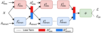
The Unified GNN Learning (Uni-GNN) framework comprises three crucial components: the structural node encoder, the semantic node encoder and the balanced node classifier. The structural node encoder is dedicated to constructing a graph adjacency matrix founded on structural connectivity, facilitating the propagation of node embeddings beyond the immediate structural neighbors of nodes. Concurrently, the semantic node encoder generates adjacency matrices based on semantic connectivity where it connects nodes to their semantically similar neighboring nodes, transcending structural distances. This facilitates the linking of nodes that are spatially distant in the graph but are from the same class, and enables message propagation between distantly located yet similar nodes, enriching the encoding process with learned node embeddings. At every layer in both the structural and semantic encoders, we propagate the integrated structural and semantic embeddings of the nodes along the corresponding connectivity, alleviating bias induced by each single type of connectivity. Ultimately, a balanced node classifier utilizes the acquired node embeddings from both the structural and semantic encoders for node classification. The overall framework of Uni-GNN is illustrated in Figure 1.
3.1.1 Structural Node Encoder
The objective of the structural encoder is to learn an embedding of the nodes based on structural connectivity. Instead of directly using the input adjacency matrix , we construct a new structural connectivity-based graph adjacency matrix that extends connections beyond the immediate neighbors in the input graph. This matrix is determined by the distances between pairs of nodes, measured in terms of the number of edges along the shortest path connecting the respective nodes, such that
| (1) |
where is the shortest path distance function that measures the distance between pairs of input nodes in terms of the number of edges along the shortest path in the input graph . The hyper-parameter governs the maximum length of the shortest path distance to be considered. In , edges connecting node pairs are assigned weights that are inversely proportional to the length of the shortest path between them. This design ensures that the propagated messages carry importance weights, scaling the messages based on the corresponding edge weights between connected nodes. The constructed structural connectivity enables us to directly propagate messages to nodes beyond a node’s immediate structural neighbors in the original graph. This is beneficial for expanding the influence of labeled minority nodes towards more distant neighboring nodes within the graph, particularly when there are under-reaching problems induced by sparse connectivities in the original graph.
The structural node encoder, denoted as , consists of message propagation layers. In each layer of the structural node encoder, denoted as , the node input features comprise the learned node embeddings, and , from the previous layer of both the structural encoder and the semantic encoder, respectively. As a consequence, the propagated messages encode both semantic and structural information facilitating the learning of more discriminative node embeddings. The constructed structural connectivity matrix is employed as the adjacency matrix for message propagation within each layer. We employ the conventional Graph Convolution Network (GCN) (Kipf & Welling, 2017) as our message-passing layer, given its simplicity, efficiency and ability to handle weighted graph structures, in the following manner:
| (2) | ||||
Here, represents the non-linear activation function, denotes the feature concatenation operation, is the matrix of learnable parameters for , is the adjusted adjacency matrix with self-connections, and is the diagonal node degree matrix of such that . In the case of the first layer of , the node input features are solely represented by the input feature matrix .
3.1.2 Semantic Node Encoder
The objective of the semantic node encoder is to learn node embeddings based on the semantic connectivity. The semantic node encoder, denoted as , comprises message passing layers. In each layer of the semantic node encoder, represented by , a semantic-based graph adjacency matrix is constructed based on the similarity between the embeddings of nodes from the previous layer of the semantic and structural node encoders, measured in terms of clustering assignments. For each layer , the following fine-grained node clustering is performed:
| (3) |
which clusters all the graph nodes into () clusters. Here, is the fine-grained clustering assignment matrix obtained from the clustering function . The row indicates the cluster to which node is assigned. The fine-grained clustering function takes as input the concatenation of the structural and semantic node embeddings from layer , along with the number of clusters , and outputs the cluster assignments . The clustering function is realized by performing K-means clustering to minimize the following least squares clustering loss:
| (4) |
where represents the mean vector for the cluster , and has a binary value (0 or 1) that indicates whether node is assigned to cluster . Based on the fine-grained clustering assignment matrix , the construction of the semantic connectivity-based graph adjacency matrix is detailed as follows:
| (5) |
In the construction of , nodes assigned to the same cluster are connected, establishing edges between them, while nodes assigned to different clusters are not connected, resulting in an adjacency matrix that encapsulates the semantic connectivity encoded within the fine-grained clusters. This process enables message propagation among nodes that share semantic similarities in the graph, irrespective of their structural separation. This is instrumental in addressing the issue of under-reaching of minority nodes. Moreover, by constructing individual semantic adjacency matrix for each layer, we can prevent adherence to fixed local semantic clusters and enhance both robustness and adaptivity. The semantic connectivity matrix of the first layer of the semantic encoder, , is constructed based on the input features matrix . Furthermore, to balance efficiency with stability during the training process, an update mechanism is introduced. Specifically, is periodically updated by re-clustering the nodes based on the updated node embeddings along the training process. The update is performed at intervals of training iterations. This adaptive strategy ensures that the semantic connectivity information remains relevant and adapts to the evolving node embeddings during the training process.
Each layer of the semantic node encoder, , takes the concatenation of node embeddings, , from the previous layer of both the structural encoder and the semantic encoder as input, aiming to gather richer information from both aspects, but propagates messages with the constructed semantic adjacency matrix . For the first layer of , the input node features are simply the input features matrix . We opt for the conventional Graph Convolution Network (GCN) (Kipf & Welling, 2017) as our message-passing layer again, which is employed in the following manner:
| (6) | ||||
Here, again represents the non-linear activation function; is the matrix of learnable parameters for ; is the adjusted adjacency matrix with self-connections; and the diagonal node degree matrix is computed as .
3.1.3 Balanced Node Classifier
We define a balanced node classification function , which classifies the nodes in the graph based on their structural and semantic embeddings learned by the Structural Encoder and Semantic Encoder respectively. In particular, the balanced node classification function takes as input the output of the -th layers of the structural and semantic node encoders, denoted as and , respectively:
| (7) |
where is the predicted class probability matrix of all the nodes in the graph. Given the class imbalance in the set of labeled nodes , the node classification function is trained to minimize the following weighted node classification loss on the labeled nodes:
| (8) |
Here, denotes the standard cross-entropy loss function. For a given node , represents its predicted class probability vector, and is the true label indicator vector if is a labeled node. The weight associated with each node is introduced to balance the contribution of data from different classes in the supervised training loss. It gives different weights to nodes from different classes. In particular, the class balance weight is calculated as follows:
| (9) |
where denotes the class index of node , such that ; and is the size of class in the labeled nodes— i.e., the number of labeled nodes from class . Since is inversely proportional to the corresponding class size, it enforces that larger weights are assigned to nodes from minority classes with fewer labeled instances in the supervised node classification loss, while smaller weights are assigned to nodes from majority classes with abundant labeled nodes. Specifically, through the incorporation of this class weighting mechanism, each class contributes equally to the supervised loss function, irrespective of the quantity of labeled nodes associated with it within the training set, thereby promoting balanced learning across different classes.
| # Min. Class | 3 | 5 | |||||||||||
|---|---|---|---|---|---|---|---|---|---|---|---|---|---|
| 10% | 5% | 10% | 5% | ||||||||||
| bAcc. | Macro-F1 | G-Means | bAcc. | Macro-F1 | G-Means | bAcc. | Macro-F1 | G-Means | bAcc. | Macro-F1 | G-Means | ||
| Cora | GCN | ||||||||||||
| Over-sampling | |||||||||||||
| Re-weight | |||||||||||||
| SMOTE | |||||||||||||
| Embed-SMOTE | |||||||||||||
| GraphSMOTE | |||||||||||||
| GraphENS | |||||||||||||
| LTE4G | |||||||||||||
| Uni-GNN | |||||||||||||
| CiteSeer | GCN | ||||||||||||
| Over-sampling | |||||||||||||
| Re-weight | |||||||||||||
| SMOTE | |||||||||||||
| Embed-SMOTE | |||||||||||||
| GraphSMOTE | |||||||||||||
| GraphENS | |||||||||||||
| LTE4G | |||||||||||||
| Uni-GNN | |||||||||||||
| # Min. Class | 1 | 2 | |||||||||||
| 10% | 5% | 10% | 5% | ||||||||||
| PubMed | GCN | ||||||||||||
| Oversampling | |||||||||||||
| Re-weight | |||||||||||||
| SMOTE | |||||||||||||
| Embed-SMOTE | |||||||||||||
| GraphSMOTE | OOM | OOM | OOM | OOM | OOM | OOM | OOM | OOM | OOM | OOM | OOM | OOM | |
| LTE4G | |||||||||||||
| Uni-GNN | |||||||||||||
3.2 Balanced Pseudo-Label Generation
To leverage the unlabeled nodes in the graph, a balanced pseudo-label generation mechanism is proposed. The objective is to increase the number of available labeled nodes in the graph while considering the class imbalance in the set of labeled nodes. The goal is to generate more pseudo-labels from minority classes and fewer pseudo-labels from majority classes, thus balancing the class label distribution of the training data. In particular, for each class , the number of nodes to pseudo-label, denoted as , is set as the difference between the largest labeled class size and the size of class , aiming to balance the class label distribution over the union of labeled nodes and pseudo-labeled nodes:
| (10) |
The set of unlabeled nodes that can be confidently pseudo-labeled to class can be determined as:
| (11) |
where is a hyperparameter determining the confidence prediction threshold. Balanced sampling is then performed on each set by selecting the top nodes, denoted as , with the most confident pseudo-labels based on the predicted probability . This results in a total set of pseudo-labeled nodes, denoted as , from all classes:
| (12) |
The Unified GNN Learning framework is trained to minimize the following node classification loss over this set of pseudo-labeled nodes :
| (13) |
where again is the standard cross-entropy loss function, is the predicted class probability vector with classifier , and is a one-hot pseudo-label vector with a single 1 at the predicted class entry . This pseudo-labeling mechanism aims to augment the labeled node set, particularly focusing on addressing class imbalances by generating more pseudo-labels for minority classes.
Training Loss
The unified GNN Learning framework is trained on the labeled set and the selected pseudo-labeled set in an end-to-end fashion to minimize the following integrated total loss:
| (14) |
where is a hyper-parameter. The training procedure is provided in the Appendix.
4 Experiments
4.1 Experimental Setup
Datasets & Baselines
We conduct experiments on three datasets (Cora, CiteSeer and PubMed) (Sen et al., 2008). To ensure a fair comparison, we adhere to the evaluation protocol used in previous studies (Zhao et al., 2021; Yun et al., 2022). The datasets undergo manual pre-processing to achieve the desired imbalance ratio (). Specifically, each majority class is allocated 20 labeled training nodes, while each minority class is assigned labeled training nodes. For validation and test sets, each class is assigned 25 and 55 nodes, respectively. Following the protocol of (Yun et al., 2022), we consider two imbalance ratios (), and two different numbers of minority classes: 3 and 5 on Cora and CiteSeer, and 1 and 2 on the PubMed dataset. Additionally, for Cora and CiteSeer, we also adopt a long-tail class label distribution setup. Here, low-degree nodes from minority classes are removed from the graph until the desired imbalance ratio () of 1% and class label distribution are achieved, similar to (Park et al., 2021; Yun et al., 2022). We compare the proposed Uni-GNN with the underlying GCN baseline, as well as various traditional and graph-based class-imbalanced learning baselines: Over-sampling, Re-weight (Yuan & Ma, 2012), SMOTE (Chawla et al., 2002), Embed-SMOTE (Ando & Huang, 2017), GraphSMOTE (Zhao et al., 2021), GraphENS (Park et al., 2021), and LTE4G (Yun et al., 2022).
Implementation Details Graph Convolution Network (GCN) (Kipf & Welling, 2017) implements the message passing layers in our proposed framework and all the comparison baselines. The semantic and structural encoders consist of 2 message passing layers each, followed by a ReLU activation function. The node classifier is composed of a single GCN layer, followed by ReLU activation, and then a single fully connected linear layer. Uni-GNN undergoes training using an Adam optimizer with a learning rate of and weight decay of over 10,000 epochs. We incorporate an early stopping criterion with a patience of 1,000 epochs and apply a dropout rate of 0.5 to all layers of our framework. The size of the learned hidden embeddings for all layers of structural and semantic encoders is set to 64. The hyperparameter is assigned the value 1. For the hyperparameters , , , and , we explore the following ranges: , , , and , respectively. Each experiment is repeated three times, and the reported performance metrics represent the mean and standard deviation across all three runs. For results for comparison methods on Cora and CiteSeer, we refer to the outcomes from (Yun et al., 2022).
| Cora-LT | CiteSeer-LT | |||||
|---|---|---|---|---|---|---|
| bAcc. | Macro-F1 | G-Means | bAcc. | Macro-F1 | G-Means | |
| GCN | ||||||
| Over-sampling | ||||||
| Re-weight | ||||||
| SMOTE | ||||||
| Embed-SMOTE | ||||||
| GraphSMOTE | ||||||
| GraphENS | ||||||
| LTE4G | ||||||
| Uni-GNN | ||||||
4.2 Comparison Results
| (# Min. Class, ) | Cora (3, 10%) | CiteSeer (3, 10%) | Cora (LT, 1%) | CiteSeer (LT, 1%) | ||||||||
|---|---|---|---|---|---|---|---|---|---|---|---|---|
| bAcc. | Macro-F1 | G-Means | bAcc. | Macro-F1 | G-Means | bAcc. | Macro-F1 | G-Means | bAcc. | Macro-F1 | G-Means | |
| GCN | ||||||||||||
| Uni-GNN | ||||||||||||
| Ind. Enc. | ||||||||||||
| Drop | ||||||||||||
| Semantic Enc. | ||||||||||||
| Structural Enc. | ||||||||||||
| Imbalanced PL | ||||||||||||
| Fixed | ||||||||||||

We evaluate the performance of Uni-GNN framework on the semi-supervised node classification task under class imbalance. Across the three datasets, we explore four distinct evaluation setups by manipulating the number of minority classes and the imbalance ratio (). Additionally, we explore the long-tail class label distribution setting for Cora and CiteSeer with an imbalance ratio of . We assess the performance of Uni-GNN using balanced Accuracy (bAcc), Macro-F1, and Geometric Means (G-Means), reporting the mean and standard deviation of each metric over 3 runs. Table 1 summarizes the results for different numbers of minority classes and imbalance ratios on all three datasets, while Table 2 showcases the results under long-tail class label distribution on Cora and CiteSeer.
Table 1 illustrates that the performance of all methods diminishes with decreasing imbalance ratio () and increasing numbers of minority classes. Our proposed framework consistently outperforms the underlying GCN baseline and all other methods across all three datasets and various evaluation setups. The performance gains over the GCN baseline are substantial, exceeding 10% in most cases for Cora and CiteSeer datasets and 13% for most instances of the PubMed dataset. Moreover, Uni-GNN consistently demonstrates superior performance compared to all other comparison methods, achieving notable improvements over the second-best method (LTE4G) by around 3%, 5%, and 11% on Cora, CiteSeer with 3 minority classes and , and PubMed with 1 minority class and , respectively. Similarly, Table 2 highlights that Uni-GNN consistently enhances the performance of the underlying GCN baseline, achieving performance gains exceeding 8% and 12% on Cora-LT and CiteSeer-LT datasets, respectively. Furthermore, Uni-GNN demonstrates remarkable performance gains over all other class imbalance methods, surpassing 3% and 6% on Cora-LT and CiteSeer-LT, respectively. These results underscore the superior performance of our framework over existing state-of-the-art class-imbalanced GNN methods across numerous challenging class imbalance scenarios.
4.3 Ablation Study
We conducted an ablation study to discern the individual contributions of each component in our proposed framework. In addition to the underlying GCN baseline, eight variants were considered: (1) Independent Node Encoders (Ind. Enc.): each node encoder exclusively propagates its own node embeddings, instead of propagating the concatenated semantic and structural embeddings. Specifically, solely propagates while solely propagates . (2) Drop : excluding the balanced pseudo-label generation. (3) : structural connectivity considers only immediate neighbors of nodes (). (4) Semantic Encoder only (Semantic Enc.): it discards the structural encoder. (5) Structural Encoder only (Structural Enc.): it discards the semantic encoder. (6) Imbalanced Pseudo-Labeling: it generates pseudo-labels for all unlabeled nodes with confident predictions without considering class imbalance. (7) Fixed : it does not update the semantic connectivity during training. (8) : it assigns equal weights to all labeled nodes in the training set. Evaluation was performed on Cora and CiteSeer datasets, each with 3 minority classes and imbalance ratio () of 10%, and with long-tail class label distribution and imbalance ratio () of 1%. The results are reported in Table 3.
Table 3 illustrates performance degradation in all variants compared to the full proposed framework. The observed performance decline in the Independent Node Encoders (Ind. Enc.) variant underscores the importance of simultaneously propagating semantic and structural embeddings across both the semantic and structural connectivity. This emphasizes the need for incorporating both aspects to effectively learn more discriminative node embeddings. The performance drop observed in the Semantic Enc. and Structural Enc. variants underscores the significance and individual contribution of each connectivity type to the proposed Uni-GNN framework. This highlights the critical role that each type of connectivity plays in the overall performance of the proposed framework. The variant’s performance drop emphasizes the importance of connecting nodes beyond their immediate structural neighbors, enabling the propagation of messages across a larger portion of the graph and learning more discriminative embeddings. The performance degradation in Drop and Imbalanced Pseudo-Labeling variants validates the substantial contribution of our balanced pseudo-label generation mechanism. The variant underscores the importance of assigning weights to each node in the labeled training set based on their class frequency. The consistent performance drops across both datasets for all variants affirm the essential contribution of each corresponding component in the proposed framework.
4.4 Hyper-Parameter Sensitivity
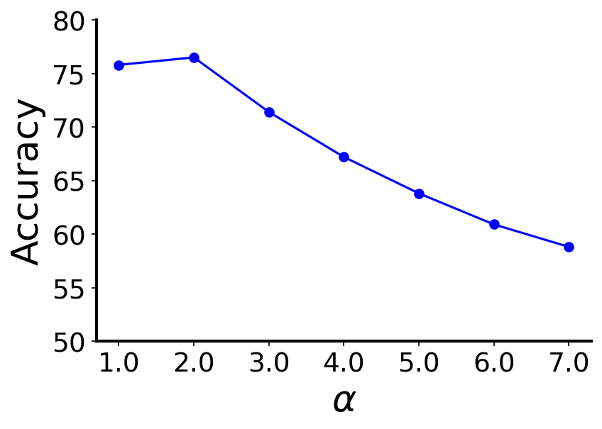
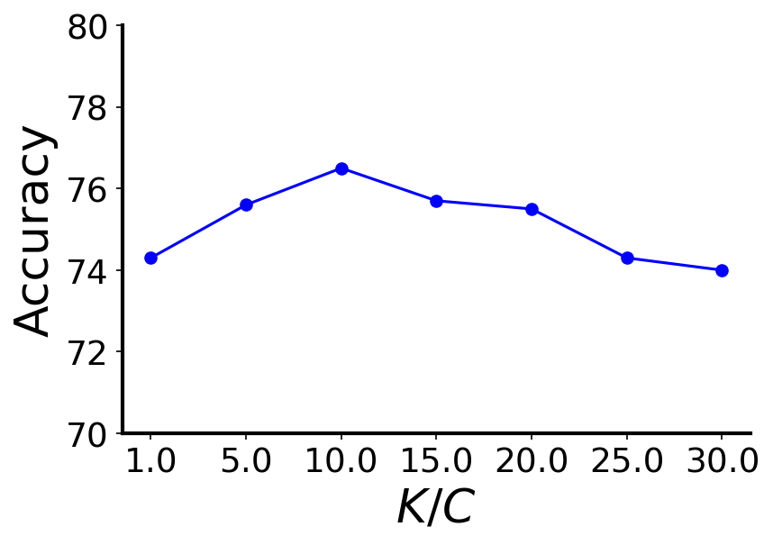
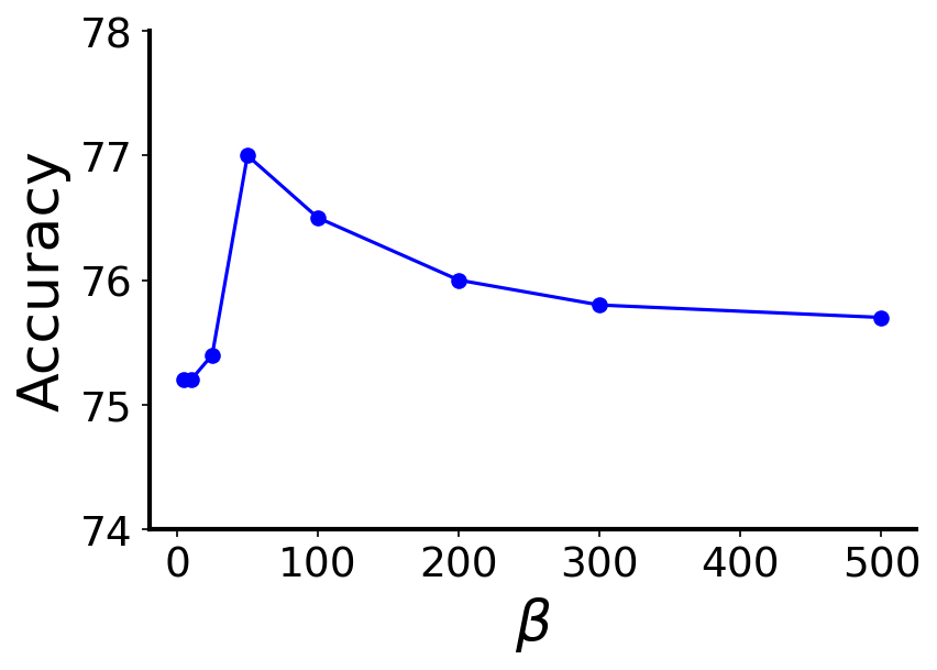
To investigate the impact of the hyper-parameters in Uni-GNN framework, we present the results of several sensitivity analyses on the Cora dataset with 3 minority classes and an imbalance ratio of 10% in Figure 2. Figures 2(a), 2(b), 2(c), and 2(d) depict the accuracy of Uni-GNN as we independently vary the max SPD distance in (), the number of clusters (), the pseudo-label confidence threshold () and the rate of updating (), respectively. Larger values for result in performance degradation due to over-smoothing as the graph becomes more densely connected. Optimal performance is achieved with . Uni-GNN exhibits robustness to variations in the hyperparameters , , and within a broad range. It consistently outperforms state-of-the-art methods across diverse settings of these hyperparameters, as depicted by the corresponding results presented in Table 1. Small values lead to noisy clusters with mixed-class nodes, while large values result in over-segmented clusters with sparse semantic connectivity. Optimal performance is achieved when falls within the range of to . Inadequately small values for result in the utilization of noisy pseudo-label predictions in the training process, while excessively large values exclude reasonably confident pseudo-labeled nodes from selection. The optimal range for lies between 0.4 and 0.7. Extremely small values for lead to frequent updates of the semantic connectivity, preventing Uni-GNN from learning stable discriminative embeddings. Values around 100 training epochs yield the best results.
5 Conclusion
In this paper, we introduced a novel Uni-GNN framework for class-imbalanced node classification. The proposed framework harnesses the combined strength of structural and semantic connectivity through dedicated structural and semantic node encoders, enabling the learning of a unified node representation. By utilizing these encoders, the structural and semantic connectivity ensures effective propagation of messages well beyond the structural immediate neighbors of nodes, thereby addressing the under-reaching and neighborhood memorization problems. Moreover, we proposed a balanced pseudo-label generation mechanism to incorporate confident pseudo-label predictions from minority unlabeled nodes into the training set. Our experimental evaluations on three benchmark datasets for node classification affirm the efficacy of our proposed framework. The results demonstrate that Uni-GNN adeptly mitigates class imbalance bias, surpassing existing state-of-the-art methods in class-imbalanced graph learning.
References
- Ahn et al. (2023) Ahn, S., Ko, J., and Yun, S.-Y. Cuda: Curriculum of data augmentation for long-tailed recognition. In International Conference on Learning Representations (ICLR), 2023.
- Ando & Huang (2017) Ando, S. and Huang, C. Y. Deep over-sampling framework for classifying imbalanced data. In European Conf. on Machine Learn. and Principles and Practice of Knowledge Dis. in Databases (ECML PKDD), 2017.
- Chawla et al. (2002) Chawla, N. V., Bowyer, K. W., Hall, L. O., and Kegelmeyer, W. P. Smote: synthetic minority over-sampling technique. In Journal of Artificial Intelligence Research, 2002.
- Hamilton et al. (2017) Hamilton, W., Ying, Z., and Leskovec, J. Inductive representation learning on large graphs. In Advances in Neural Information Processing Systems (NIPS), 2017.
- Hao et al. (2020) Hao, Z., Lu, C., Huang, Z., Wang, H., Hu, Z., Liu, Q., Chen, E., and Lee, C. Asgn: An active semi-supervised graph neural network for molecular property prediction. In SIGKDD International Conference on Knowledge Discovery & Data Mining (KDD), 2020.
- Kim et al. (2020) Kim, J., Jeong, J., and Shin, J. M2m: Imbalanced classification via major-to-minor translation. In Conference on Computer Vision and Pattern Recognition (CVPR), 2020.
- Kipf & Welling (2017) Kipf, T. N. and Welling, M. Semi-supervised classification with graph convolutional networks. In Inter. Conference on Learning Representations (ICLR), 2017.
- Li et al. (2023) Li, W.-Z., Wang, C.-D., Xiong, H., and Lai, J.-H. Graphsha: Synthesizing harder samples for class-imbalanced node classification. In SIGKDD Conference on Knowledge Discovery and Data Mining (KDD), 2023.
- Mahajan et al. (2018) Mahajan, D., Girshick, R., Ramanathan, V., He, K., Paluri, M., Li, Y., Bharambe, A., and Van Der Maaten, L. Exploring the limits of weakly supervised pretraining. In European conference on Computer Vision (ECCV), 2018.
- Menon et al. (2021) Menon, A. K., Jayasumana, S., Rawat, A. S., Jain, H., Veit, A., and Kumar, S. Long-tail learning via logit adjustment. In International Conference on Learning Representations (ICLR), 2021.
- Park et al. (2021) Park, J., Song, J., and Yang, E. Graphens: Neighbor-aware ego network synthesis for class-imbalanced node classification. In International Conference on Learning Representations (ICLR), 2021.
- Qu et al. (2021) Qu, L., Zhu, H., Zheng, R., Shi, Y., and Yin, H. Imgagn: Imbalanced network embedding via generative adversarial graph networks. In SIGKDD Conf. on Knowledge Discovery & Data Mining (KDD), 2021.
- Ren et al. (2020) Ren, J., Yu, C., Ma, X., Zhao, H., Yi, S., et al. Balanced meta-softmax for long-tailed visual recognition. In Advances in Neural Information Processing Systems (NeurIPS), 2020.
- Sen et al. (2008) Sen, P., Namata, G., Bilgic, M., Getoor, L., Galligher, B., and Eliassi-Rad, T. Collective classification in network data. In AI magazine, 2008.
- Song et al. (2022) Song, J., Park, J., and Yang, E. Tam: topology-aware margin loss for class-imbalanced node classification. In International Conference on Machine Learning (ICML), 2022.
- Sun et al. (2022) Sun, Q., Li, J., Yuan, H., Fu, X., Peng, H., Ji, C., Li, Q., and Yu, P. S. Position-aware structure learning for graph topology-imbalance by relieving under-reaching and over-squashing. In International Conference on Information & Knowledge Management (CIKM), 2022.
- Tang et al. (2020) Tang, X., Yao, H., Sun, Y., Wang, Y., Tang, J., Aggarwal, C., Mitra, P., and Wang, S. Investigating and mitigating degree-related biases in graph convoltuional networks. In International Conference on Information & Knowledge Management (CIKM), 2020.
- Veličković et al. (2018) Veličković, P., Cucurull, G., Casanova, A., Romero, A., Liò, P., and Bengio, Y. Graph attention networks. In International Conference on Learning Representations (ICLR), 2018.
- Wallace et al. (2011) Wallace, B. C., Small, K., Brodley, C. E., and Trikalinos, T. A. Class imbalance, redux. In International Conference on Data Mining (ICDM), 2011.
- Wang et al. (2022) Wang, K., An, J., Zhou, M., Shi, Z., Shi, X., and Kang, Q. Minority-weighted graph neural network for imbalanced node classification in social networks of internet of people. In IEEE Internet of Things Journal, 2022.
- Wang et al. (2023) Wang, S., Zeng, Z., Yang, X., and Zhang, X. Self-supervised graph learning for long-tailed cognitive diagnosis. In AAAI Conf. on Artificial Intelligence, 2023.
- Wei et al. (2021) Wei, C., Sohn, K., Mellina, C., Yuille, A., and Yang, F. Crest: A class-rebalancing self-training framework for imbalanced semi-supervised learning. In Conference on Computer Vision and Pattern Recognition (CVPR), 2021.
- Yan et al. (2023) Yan, L., Zhang, S., Li, B., Zhou, M., and Huang, Z. Unreal: Unlabeled nodes retrieval and labeling for heavily-imbalanced node classification. In arXiv preprint arXiv:2303.10371, 2023.
- Yuan & Ma (2012) Yuan, B. and Ma, X. Sampling+ reweighting: Boosting the performance of adaboost on imbalanced datasets. In International Joint Conference on Neural Networks (IJCNN), 2012.
- Yun et al. (2022) Yun, S., Kim, K., Yoon, K., and Park, C. Lte4g: long-tail experts for graph neural networks. In International Conference on Information & Knowledge Management (CIKM), 2022.
- Zhang et al. (2021) Zhang, G., Wu, J., Yang, J., Beheshti, A., Xue, S., Zhou, C., and Sheng, Q. Z. Fraudre: Fraud detection dual-resistant to graph inconsistency and imbalance. In International Conference on Data Mining (ICDM), 2021.
- Zhao et al. (2021) Zhao, T., Zhang, X., and Wang, S. Graphsmote: Imbalanced node classification on graphs with graph neural networks. In International conference on web search and data mining (WSDM), 2021.
- Zhong et al. (2021) Zhong, Z., Cui, J., Liu, S., and Jia, J. Improving calibration for long-tailed recognition. In Conf. on Computer Vision and Pattern Recognition (CVPR), 2021.
Appendix A Training Procedure
The details of the training procedure of the Unified GNN Learning framework are presented in algorithm 2.
Appendix B Datasets
The specifics of the benchmark datasets are detailed in Table 4. Detailed class label distribution information for the training sets in all evaluation setups on all datasets are provided in Table 5.
| Dataset | # Nodes | # Edges | # Features | # Classes |
|---|---|---|---|---|
| Cora | 2,708 | 5,278 | 1,433 | 7 |
| CiteSeer | 3,327 | 4,552 | 3,703 | 6 |
| PubMed | 19,717 | 44,324 | 500 | 3 |
| Dataset | # Min. Class | ||||||||
|---|---|---|---|---|---|---|---|---|---|
| Cora | 3 | 10% | 20 | 20 | 20 | 20 | 2 | 2 | 2 |
| 5% | 20 | 20 | 20 | 20 | 1 | 1 | 1 | ||
| 5 | 10% | 20 | 20 | 2 | 2 | 2 | 2 | 2 | |
| 5% | 20 | 20 | 1 | 1 | 1 | 1 | 1 | ||
| LT | 1% | 341 | 158 | 73 | 34 | 15 | 7 | 3 | |
| CiteSeer | 3 | 10% | 20 | 20 | 20 | 2 | 2 | 2 | - |
| 5% | 20 | 20 | 20 | 1 | 1 | 1 | - | ||
| 5 | 10% | 20 | 2 | 2 | 2 | 2 | 2 | - | |
| 5% | 20 | 1 | 1 | 1 | 1 | 1 | - | ||
| LT | 1% | 371 | 147 | 58 | 32 | 9 | 3 | - | |
| PubMed | 1 | 10% | 20 | 20 | 2 | - | - | - | - |
| 5% | 20 | 20 | 1 | - | - | - | - | ||
| 2 | 10% | 20 | 2 | 2 | - | - | - | - | |
| 5% | 20 | 1 | 1 | - | - | - | - |