Out-of-equilibrium Monte Carlo simulations of a classical gas with Bose-Einstein statistics
Abstract
Algorithms to determine transition probabilities in Monte Carlo simulations are tested using a system of classical particles with effective interactions which reproduce Bose-Einstein statistics. The system is appropriate for testing different Monte Carlo simulation methods in out-of-equilibrium situations since non equivalent results are produced. We compare mobility numerical results obtained with transition probabilities derived from Glauber and Metropolis algorithms. Then, we compare these with a recent method, the interpolation algorithm, appropriate for non-equilibrium systems in homogeneous substrata and without phase transitions. The results of mobility obtained from the interpolation algorithm are qualitatively verified with molecular dynamics simulations for low concentrations.
I Introduction
If transition probabilities between different states of a system are known, then the kinetic Monte Carlo algorithm can be used to numerically reproduce a correct description of the transient or non-equilibrium behavior Bortz et al. (1975); Fichthorn and Weinberg (1991); Voter (2005); Jansen (2012). Nevertheless, it is not uncommon that the information available is restricted to the state’s energy, and transition probabilities have to be estimated using, for example, Glauber or Metropolis algorithms. Such algorithms guarantee a correct description of the equilibrium state, but not of the out-of-equilibrium transient. Convergence towards equilibrium is ensured by imposing the detailed balance condition on the transition probabilities, see for example Binder (1997); Binder and Heermann (2010).
Let us consider a system of particles, at temperature , divided into cells; transition probabilities describe jumps of one particle between neighboring cells. In Refs. Suárez et al. (2015); Martínez and Hoyuelos (2018, 2019a), it has been shown that the detailed balance condition can be used to derive a class of transition probabilities characterized by an interpolation parameter . If , the transition probability depends on the one-particle potential in the origin cell; if , it depends on the potential in the target cell; and if , it depends on the potential energy change (a frequent choice in Monte Carlo simulations). The interpolation algorithm consists in the implementation of the kinetic Monte Carlo method using transition probabilities that are obtained from the potential and the interpolation parameter Suárez et al. (2015); Martínez and Hoyuelos (2018, 2019a). The purpose of this paper is to verify that this algorithm correctly describes an out-of-equilibrium system. To do this we select a specific example. The chosen system is a gas of classical particles with an effective attractive interaction which reproduces Bose-Einstein statistics. The main reason for this choice is that this system exhibits clear differences among the results generated by the mentioned numerical algorithms, in contrast, as shown below, with purely repulsive interaction of hard core.
So, we consider the following stationary non-equilibrium state. A constant force is applied along direction ; the external potential is , where is the position of cell . The system has periodic boundary conditions along the axis and, after some time, a stationary current is established. Particles have a mean velocity proportional to and the proportionality constant is the mobility . We consider (for small values of ) as the parameter which characterizes the non-equilibrium state, and analyze its dependence on the density for the different algorithms.
This article is organized as follows. In Sec. II, the three algorithms used for transition probabilities: Glauber, Metropolis and interpolation, are described. In Sec. III, the hard-core interaction is briefly analyzed. In Sec. IV, the basic formulae for the Bose-Einstein gas are derived. In Sec. V, we present numerical and analytical results of the mobility using Glauber, Metropolis and interpolation algorithms for the Bose-Einstein gas. The Monte Carlo simulations are performed in a one-dimensional lattice gas with periodic boundary conditions. For completeness and as a verification, in Sec. VI, we compare the previous results with the ones obtained through Molecular Dynamics. This corresponds to a more detailed kinetic description, where the position and velocity of each particle inside the cells are considered sup Finally, conclusions are presented in Sec. VII.
II Algorithms for transition probabilities
According to the Glauber algorithm Glauber (1963), in a Monte Carlo step the transition from state to state , with energies and respectively, has a probability
| (1) |
where .
In the Metropolis or Metropolis-Hastings algorithm Hastings (1970), the probability is
| (2) |
Note that Metropolis algorithm is faster: if , we have and . We have to take this difference into account to have the same time scale in both cases. If is the number of jump attempts per unit time, then the transition probabilities are
| (3) | ||||
| (4) |
where a factor 2 is included in to compensate the speed difference between algorithms.
The energy of a given configuration is
| (5) |
where represents the interaction energy (or configuration energy) among the particles in the cell, in local equilibrium, and is an external potential. Only processes where one particle jumps to a neighboring cell are allowed.
A different perspective is adopted for the interpolation algorithm. Instead of using the state energy, the mean field potential for one particle, produced by all the other particles in the cell, is considered. We call the interpolation parameter in cell . The transition probability from cell to cell is given by
| (6) |
where and . See Ref. Vattulainen et al. (1998) for a related approach in which the transition probability depends on the sum of energies in origin and target sites. Note that and can be functions of the number of particles, , in a cell .
A relationship between and has to be established. This can be done using the equilibrium distribution of particles . From the transition probabilities (6), a Fokker-Planck equation can be derived, whose equilibrium solution is
| (7) |
where is the chemical potential, see Ref. Suárez et al. (2015). On the other hand, can also be obtained from the grand partition function for cell with energy . Combining both results, it can be shown Suárez et al. (2015) that
| (8) |
where is evaluated at the average number ( is a continuous function of but, when implementing the algorithm for specific realizations, has to be evaluated only at integer values of ).
The interpolation parameter can be simplified in the definition of transition probabilities (6) using the following relationship that holds in the absence of a phase transition:
| (9) |
where is the the derivative of with respect to the number of particles. The demonstration of (9) can be found in Ref. Martínez and Hoyuelos (2019b); it is obtained from the fact that the energy difference between final and initial states is equal to the difference between the energy barriers (the exponents in ) of the forward and backward processes. The transition probability form cell to becomes
| (10) |
In summary, transition probabilities in the interpolation algorithm are not obtained directly from the state energy, but are functions of the potential that is obtained from (8). The method is more involved than Glauber or Metropolis, and it only applies to system of particles with local interactions, where the energy can be written as in (5). The advantage is that it holds out of equilibrium.
Here, models where is a simple function of are considered. Long range interactions, such as the Coulomb potential, can not be represented by these methods, where the energy of one cell, given by , does not depend on the number of particles in nearby cells. Interaction between particles in different cells is neglected. For a specific (short range) interaction potential, the configuration energy in general has to be obtained numerically. If the interaction potential is , with the position of particles in cell , the configuration energy is given by
| (11) |
where average is computed with the probability distribution of non-interacting particles (that is, particles randomly distributed).
III Hard-core interaction
The main purpose of this paper is to check the different algorithms with an effective Bose-Einstein interaction. But before that, we wish to briefly analyze other simple potential: hard core. These potentials represent two extreme situations: purely attractive or purely repulsive interactions. It is shown in this section that the mobility of hard spheres against concentration is the same independently of the simulation algorithm. Any of the three options, Glauber, Metropolis or interpolation, can be used for the description of the out-of-equilibrium behavior of hard spheres in a discrete lattice.
The hard-core interaction is given by
| (12) |
Hard core imposes that, in any cell, takes values 0 or 1 only. Let us consider a jump from cell to cell . The energy of the initial configuration is , and the energy of the final configuration is . The external energy change is , with the cell size. Then, the energy change is
| (15) |
where it was assumed that so that the jump process from to is possible (there must be a particle to make the jump).
Let us call the mean velocity of particles when a force is applied. Analytical expressions for the mobility, defined as , can be derived for the three algorithms to compare with numerical results. Mobility is obtained from the mean current:
| (16) |
since , so that . We call the mobilities for Glauber and Metropolis algorithms and respectively. In the ideal system, where effects of interactions are neglected, the mobility is given by the Einstein relation: , where is the diffusivity.
First, for the Metropolis algorithm, the transition probability for a jump from to , assuming that , is
| (17) |
expression that can be written as
| (18) |
And, for the jump from to ,
| (19) |
where it is assumed that the force and the cell size satisfy so that ; this approximation is necessary to get a linear relation between mean velocity and force , from which the mobility is obtained; the approximation corresponds to the linear regime of non equilibrium thermodynamics. Using (18) and (19) to evaluate the current (16), we get
| (20) |
and the mobility is
| (21) |
It is convenient to present the mobility relative to , so that the result is independent of the jump rate or the cell size . In the last expressions, subindex is not used for the mean number of particles, , since a homogeneous system is considered.
For the Glauber algorithm, using the definition (1), it can be shown that
| (22) | ||||
| (23) |
Using (16), the result for the current turns out to be equal to , and, of course, also the mobility:
| (24) |
For the interpolation algorithm, the first step is to calculate . We have that
| (27) | ||||
| (28) |
then, from Eq. (8), we have
| (29) |
and
| (30) |
When replacing this expressions in Eq. (10) for the transition probability, as mentioned before, and have to be evaluated at integer values of . Then, using also that
| (31) |
it can be shown that the transition probabilities for the interpolation algorithm are equal to those of the Glauber algorithm:
| (32) | ||||
| (33) |
Therefore, the mobility is also the same,
| (34) |
Figure 1 shows numerical results of the mobility using Metropolis and Glauber (or interpolation) algorithms for the hard-core interaction. The results match the expression obtained for .

In summary, hard spheres are not useful to discriminate among algorithms. Any of them seems to work. This is not the case for the attractive interaction of a classical Bose-Einstein gas, and this is the main reason why we focus our attention on it.
IV Basic formulae for the Bose-Einstein gas
In the lattice gas description, the system is divided into cells of size much smaller than the characteristic length of particle density variations. Temperature and chemical potential are homogeneous. Interaction energy between particles in different cells is neglected. Since spatial variations are smooth, cells are point-like in the continuous limit, and local thermal equilibrium holds. This means that each cell can be considered as an equilibrium system, although the whole system is out of equilibrium. We can write the classical grand partition function of cell as
| (35) |
where the energy in cell is .
We consider a configuration energy
| (36) |
to reproduce Bose-Einstein statistics, since in this case we have
| (37) |
and the average number of particles is
| (38) |
If we know that the system has a total number of particles , the chemical potential is obtained from the relationship , where the sum is performed in all cells. From Ec. (38), the chemical potential is
| (39) |
Let us consider a cell in which the potential takes a value , i.e. a reference chemical potential. Then, in the previous expression, we can recognize the ideal and residual parts of the chemical potential:
| (40) |
This simplified description in terms of jumps between neighboring cells is intended to correctly reproduce the behavior of a system of particles which move with given velocities and interact with a space dependent potential. The effective potential, also known as statistical potential, between two bosons at distance is
| (41) |
where determines the range of the interaction (it is equal to the de Broglie wavelength in the quantum case) (Pathria and Beale, 2011, p. 138). Notice that here we use the term “boson” to informally refer to classical particles with Bose-Einstein statistics. The statistical potential holds for small concentration, so we can expect descriptions to agree only in this limit. The concentration of a cell (in local equilibrium) is . Also, in the limit of small concentration, we can use the cluster expansion to obtain the chemical potential:
| (42) |
where is the coefficient of two-particle clusters given by
| (43) |
see for example Eq. (5.32) in Ref. Kardar (2007). The cluster expansion is based on the quantity as a convenient expansion parameter, with the interaction potential. For short-range hard-core interactions, it is equal to for and decays to zero for increasing . In our case, it takes the value for and vanishes exponentially as increases.
From Eqs. (42) and (43) we have that the chemical potential is
| (44) |
where, as in Eq. (40), we can identify the ideal and residual parts.
By imposing the condition in which the chemical potential in the lattice gas description, Eq. (40), is equal to the chemical potential in the kinetic description, Eq. (44), more specifically, by matching the residual parts of the chemical potential, we have that , and therefore,
| (45) |
But setting this condition poses a problem in the calculation of the grand partition function, since in Eq. (35) interactions with particles in neighboring cells are neglected. This approximation is valid as long as is much larger than the interaction range, i.e. , a condition that is not fulfilled in (45). Still, the qualitative behavior of the chemical potential is the same in both descriptions. We expect equivalent qualitative behaviors also for the mobility although, due to the inconsistency of approximations, we can not expect quantitative agreement.
V Mobility from Glauber, Metropolis and interpolation algorithms
The energy change for a jump from cell to with effective Bose-Einstein interaction is
| (46) |
where the condition has to be fulfilled in order to have the possibility of a jump from cell (for cells with there is no jump process and no need to calculate ).
With fixed boundary conditions and an external force, particles accumulate on one side of the system and, in equilibrium, they have the Bose-Einstein distribution given by Eq. (38). We have verified that Metropolis or Glauber algorithms converge to the Bose Einstein distribution in this case, as shown in Fig. 2.

Now we turn to the non-equilibrium situation. Instead of fixed boundary conditions, let us consider periodic boundary conditions. After some time, the system is in a stationary non-equilibrium state. The mean velocity of a particle in terms of the transition probabilities between cells of size is
| (47) |
For small concentration (ideal gas), interactions can be neglected and . It can be shown that for both algorithms, Glauber and Metropolis, the mean velocity for small concentration is . For Metropolis at small concentration and a positive force , transition probabilities are
Replacing in (47), we obtain
For the Glauber algorithm we have
And, again, replacing in (47), we obtain
The mobility, , is defined as . The previous results for the velocity, for both algorithms, are consistent with the Einstein relation; in both cases, is obtained. Subindex 0 identifies the small concentration regime.
As mentioned before, mobility is obtained from the mean current, Eq. (16). It can be shown that, for the Glauber algorithm,
| (48) |
and that the corresponding expression for the Metropolis algorithm can be simplified to
| (49) |
see the Appendix for details.
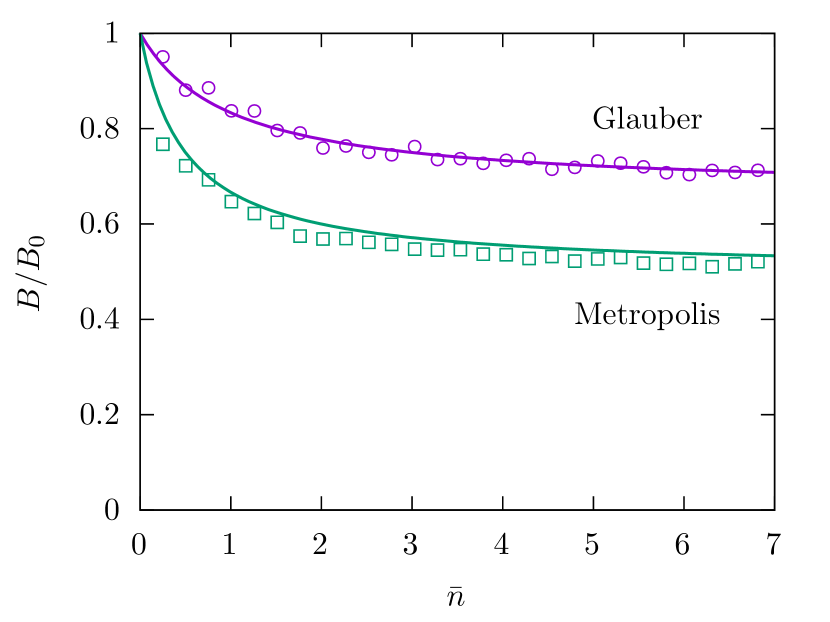
In Fig. 3, we show the numerical results of the mobility obtained with both algorithms, compared with the analytical expressions (V) and (49). The agreement between numerical and analytical results supports their validity. Both algorithms coincide in the limit of small concentration, where and interactions can be neglected. But as the mean number of particles is increased, discrepancies grow. There is a quantitative difference of about 30% between both predictions of for larger . It is well known that we can not expect a correct description of a non-equilibrium state with these algorithms. Nevertheless, it is interesting to determine how far from the correct result they are. This is the purpose of the next paragraphs.
For the interpolation algorithm, using Eq. (36) for in (8), we have
| (50) |
Notice that is equal to the residual part of the chemical potential, see Eq. (40), and Eq. (8) corresponds to the Widom insertion method, where is the insertion energy, i.e. the interaction energy needed to insert one particle. Using this result for , and its derivative, in (10), the transition probability is
| (51) |
With this information, we can calculate the mobility for the interpolation algorithm (see the Appendix). The result is
| (52) |
As in the previous results, a homogeneous system, in which , is considered for the calculation of mobility. Figure 4 shows a good agreement between this theoretical result and kinetic Monte Carlo simulations.

The result for the mobility obtained with the interpolation algorithm is qualitatively different from the results of Glauber and Metropolis algorithms. While for the interpolation algorithm we have a mobility which increases with , for the other algorithms it decreases (see Fig. 3). As mentioned before, we know that Glauber and Metropolis algorithms are designed to give the correct equilibrium state; they should not be applied to non-equilibrium situations, but it is interesting to evaluate the error. According to the interpolation algorithm, which is designed for non-equilibrium states (with limitations that are summarized in the conclusions), the error increases with concentration. Glauber and Metropolis algorithms give the correct result for the mobility only in the limit of small , where interactions can be neglected.
VI Molecular dynamics
The objective of this section is to obtain the mobility of a boson gas in the context of a classical kinetic description which includes velocity of particles, and compare with the results of the previous sections.
The method is to numerically obtain the self-diffusivity and use the Einstein relation to calculate the mobility . The Green-Kubo formula (see for example (Kubo et al., 1998, Sec. 4.6.2) or (Reichl, 1998, Sec. S10.G)) is used to obtain the self-diffusivity from the velocity autocorrelation function:
| (53) |
We wish to emphasize that with this method the mobility is obtained from simulations of the system in equilibrium, without a force applied. The main purpose of this paper is to check algorithms for Monte Carlo simulations out of equilibrium. The motivation of this section is to obtain mobility using molecular dynamics, and in this context we can choose the method based on simplicity.
To compare with results of the previous sections, we have to calculate the mobility relative to its value for the ideal gas, . From the kinetic theory of transport in dilute gases (see for example (McQuarrie, 2000, Sec. 16-1)), we know that the self-diffusivity in the ideal case, and therefore , behaves as , where is the particle density. The proportionality constant, between and , is numerically set in our results so as to have for .
Then, we perform molecular dynamic simulations of a system of particles with a given density , in equilibrium, which interact among them with the statistical potential of Eq. (41). We do this for different densities and obtain the mobility through the velocity autocorrelation function. We focus our attention on the slope of the mobility for small concentrations, since this is the limit for which the statistical potential (41) holds.

VII Conclusions
We study mobility in a system of classical particles with interactions. Two different approaches are possible: a lattice gas with transition probabilities among cells, or a kinetic description in a continuous space. A fundamental problem of the lattice gas description is to determine transition probabilities when only state energies are known. Monte Carlo simulations with Glauber or Metropolis algorithms correctly describe the equilibrium state but they are not supposed to hold out of equilibrium. Instead, the interpolation algorithm was recently introduced Suárez et al. (2015); Martínez and Hoyuelos (2018, 2019a, 2019b) in order to obtain transition probabilities that hold out of equilibrium; it is summarized in Eqs. (8) and (10). Limitations of the method are: the system should be in local thermal equilibrium (i.e. deviations from equilibrium have a characteristic length much larger than the cell size), no phase transition occur and the interaction is local [more precisely, the interaction energy can be written as in (5)]. Also, the information provided by the algorithm is incomplete if the jump rate has a non-trivial dependence on concentration, as it happens, for example, for diffusion in a solid Martínez and Hoyuelos (2019b).
We calculate the mobility in a non-equilibrium stationary state: a force is applied to a one-dimensional array of cells with periodic boundary conditions and homogeneous density. For hard core interaction, the same results are obtained for Glauber, Metropolis or interpolation algorithms. Instead, for an attractive potential such that the Bose-Einstein statistics is reproduced, important differences are obtained among algorithms. There is a difference of about 30% between the Glauber and Metropolis predictions for large concentration; in both cases, mobility decreases with concentration towards an asymptotic value. The mobility obtained from the interpolation algorithm qualitatively differs from the ones of the other methods. Instead of decreasing with concentration, it increases. This means an unbounded increasing error for the Glauber and Metropolis algorithms. They can be used to calculate mobility only in the limit of small concentration, where .
The lattice gas description should be consistent with the kinetic description. So, we also consider particles moving in a continuous space and interacting with a statistical potential (41) which corresponds to the Bose-Einstein distribution. The mobility obtained from molecular dynamics simulations, Fig. 5, is in qualitative agreement with the prediction of the interpolation algorithm.
Acknowledgements.
The authors acknowledge discussions with H. Mártin which were useful for the development of these ideas. This work was partially supported by Consejo Nacional de Investigaciones Científicas y Técnicas (CONICET, Argentina, PIP 112 201501 00021 CO). This work used computational resources from CCAD – Universidad Nacional de Córdoba cca , in particular the Mendieta Cluster, which is part of SNCAD – MinCyT, República Argentina.Appendix
In this appendix, the expressions (V) and (49) for the mobility for Glauber and Metropolis algorithms are derived.
Using (46) for the energy change, the transition probabilities for the Glauber algorithm are
| (54) | ||||
| (55) |
Replacing these expressions in the current , with
| (56) |
and making approximations for , we have
| (57) |
The first term of the right side cancels due to the symmetry of the homogeneous stationary state. Knowing that and that , we have
| (58) |
The probability of having particles knowing that the average value is , for the Bose-Einstein distribution, is given by
| (59) |
see for example (Pathria and Beale, 2011, p. 152). Using this probability, we obtain Eq. (V) for the mobility in the Glauber algorithm. Actually, a correction of order should be added to to use the probability which corresponds to the stationary non-equilibrium state, since Eq. (59) holds in equilibrium. But this correction cancels when only terms up to order are kept in the equation for the current.
A similar process is applied to obtain the mobility for the Metropolis algorithm. Replacing the expression (46) for in the Metropolis transition probabilities, we have
| (60) |
Assuming that and considering all possible combinations of and , we get
| (61) |
The average of this expression can be written as
| (62) |
These sums can be simplified. Replacing with , and using a symbolic manipulator such as Maxima Maxima, a Computer Algebra System , we obtain
| (63) |
Using the relationship between current and mobility, , Eq. (49) is immediately obtained.
Finally, the calculation of the mobility for the interpolation algorithm is simpler. We have the transition probabilities in (51), and the mean current is
| (64) |
where it was considered that and that fluctuations in different cells are independent, so . From this equation for , the result for the mobility (52) is obtained.
References
- Bortz et al. (1975) A. B. Bortz, M. H. Kalos, and J. L. Lebowitz, “A new algorithm for Monte Carlo simulation of Ising spin systems,” J. Comp. Phys. 17, 10 (1975).
- Fichthorn and Weinberg (1991) K. A. Fichthorn and W. H. Weinberg, “Theoretical foundations of dynamical Monte Carlo simulations,” J. Chem. Phys. 95, 1090 (1991).
- Voter (2005) A. F. Voter, “Introduction to the kinetic monte carlo method,” in Radiation Effects in Solids, edited by K. E. Sickafus and E. A. Kotomin (Springer, 2005).
- Jansen (2012) A. P. J. Jansen, An Introduction to Kinetic Monte Carlo Simulations of Surface Reactions (Springer, Berlin, Heidelberg, 2012).
- Binder (1997) K. Binder, “Applications of Monte Carlo methods to statistical physics,” Rep. Prog. Phys. 60, 487 (1997).
- Binder and Heermann (2010) K. Binder and D. W. Heermann, Monte Carlo Simulation in Statistical Physics (Springer, Berlin, Heidelberg, 2010).
- Suárez et al. (2015) G. Suárez, M. Hoyuelos, and H. Mártin, “Mean-field approach for diffusion of interacting particles,” Phys. Rev. E 92, 062118 (2015).
- Martínez and Hoyuelos (2018) M. Di Pietro Martínez and M. Hoyuelos, “Mean-field approach to diffusion with interaction: Darken equation and numerical validation,” Phys. Rev. E 98, 022121 (2018).
- Martínez and Hoyuelos (2019a) M. Di Pietro Martínez and M. Hoyuelos, “From diffusion experiments to mean-field theory simulations and back,” J. Stat. Mech.: Theory Exp. 2019, 113201 (2019a).
- (10) See Supplemental Material at site, which includes Refs. difcode; Large-scale Atomic/Molecular Massively Parallel Simulator ; Plimpton (1993); lammpsdoc; Pathria and Beale (2011); mdcode, for the details about the numerical implementation and the codes used to obtain the mobility results shown in this article.
- Glauber (1963) R. J. Glauber, “Time‐dependent statistics of the Ising model,” J. Math. Phys. 4, 294 (1963).
- Hastings (1970) W. K. Hastings, “Monte Carlo sampling methods using Markov chains and their applications,” Biometrika 57, 97 (1970).
- Vattulainen et al. (1998) I. Vattulainen, J. Merikoski, T. Ala-Nissila, and S. C. Ying, “Adatom dynamics and diffusion in a model of O/W(110),” Phys. Rev. B 57, 1896 (1998).
- Martínez and Hoyuelos (2019b) M. Di Pietro Martínez and M. Hoyuelos, “Diffusion in binary mixtures: an analysis of the dependence on the thermodynamic factor,” Phys. Rev. E 100, 022112 (2019b).
- Pathria and Beale (2011) R. K. Pathria and P. D. Beale, Statistical Mechanics, 3rd ed. (Elsevier, 2011).
- Kardar (2007) M. Kardar, Statistical Physics of Particles (Cambridge University Press, Cambridge, 2007).
- Kubo et al. (1998) R. Kubo, M. Toda, and N. Hashitsume, Statistical Physics II, 2nd ed. (Springer, 1998).
- Reichl (1998) L. E. Reichl, A Modem Course in Statistical Physics, 2nd ed. (Wiley, 1998).
- McQuarrie (2000) D. A. McQuarrie, Statistical Mechanics (University Science Books, Sausalito, 2000).
- (20) Large-scale Atomic/Molecular Massively Parallel Simulator, http://lammps.sandia.gov.
- Plimpton (1993) Steve Plimpton, Fast parallel algorithms for short-range molecular dynamics, Tech. Rep. (Sandia National Labs., Albuquerque, NM (United States), 1993).
- (22) CCAD – UNC: http://ccad.unc.edu.ar/.
- (23) Maxima, a Computer Algebra System, http://maxima.sourceforge.net/.