Oscillatory motions in the Restricted 3-Body Problem: A Functional Analytic Approach
Abstract.
A fundamental question in Celestial Mechanics is to analyze the possible final motions of the Restricted -body Problem, that is, to provide the qualitative description of its complete (i.e. defined for all time) orbits as time goes to infinity. According to the classification given by Chazy back in 1922, a remarkable possible behaviour is that of oscillatory motions, where the motion of the massless body is unbounded but returns infinitely often inside some bounded region:
In contrast with the other possible final motions in Chazy’s classification, oscillatory motions do not occur in the -body Problem, while they do for larger numbers of bodies. A further point of interest is their appearance in connection with the existence of chaotic dynamics.
In this paper we introduce new tools to study the existence of oscillatory motions and prove that oscillatory motions exist in a particular configuration known as the Restricted Isosceles -body Problem (RI3BP) for almost all values of the angular momentum. Our method, which is global and not limited to nearly integrable settings, extends the previous results [GPSV21] by blending variational and geometric techniques with tools from nonlinear analysis such as topological degree theory. To the best of our knowledge, the present work constitutes the first complete analytic proof of existence of oscillatory motions in a non perturbative regime.
Key words and phrases:
Restricted -body problem, parabolic motions, oscillatory motions, chaotic dynamics2020 Mathematics Subject Classification:
34C28, 37B10, 70G75 70F07, 37C83, 70K44.1. Introduction
One of the oldest questions in Dynamical Systems is to understand the mechanisms driving the global dynamics of the -body problem, which models the motion of three bodies interacting through Newtonian gravitational force. The -body Problem is called restricted if one of the bodies has mass zero and the other two have strictly positive masses. In this limit problem, the massless body is affected by, but does not affect, the motion of the massive bodies. A fundamental question concerning the global dynamics of the Restricted -body Problem is the study of its possible final motions, that is, the qualitative description of its complete (defined for all time) orbits as time goes to infinity. In 1922 Chazy gave a complete classification of the possible final motions of the Restricted -body Problem [Cha22]. To describe them we denote by the position of the massless body in a Cartesian reference frame with origin at the center of mass of the primaries.
Theorem 1.1 ([Cha22]).
Every solution of the Restricted -body Problem defined for all (future) times belongs to one of the following classes
-
•
B (bounded): .
-
•
P (parabolic) and as .
-
•
H (hyperbolic): and as .
-
•
O (oscillatory) and .
Notice that this classification also applies for . We distingish both cases adding a superindex or to each of the cases, e.g. and .
Bounded, parabolic and hyperbolic motions also exist in the -body Problem, and examples of each of these classes of motion in the Restricted -body Problem were already known by Chazy. However, the existence of oscillatory motions in the Restricted -body Problem was an open question for a long time. Their existence was first established by Sitnikov in a particular configuration of the Restricted -body Problem nowadays known as the Sitnikov problem.
1.1. The Moser approach to the existence of oscillatory motions
After Sitnikov’s work, Moser gave a new proof of the existence of oscillatory motions in the Sitnikov problem [Mos01]. His approach makes use of tools from the geometric theory of dynamical systems, in particular, hyperbolic dynamics. More concretely, Moser considered an invariant periodic orbit “at infinity” (see Section 1.3) which is degenerate (the linearized vector field vanishes) but posseses stable and unstable invariant manifolds. Then, he proved that its stable and unstable manifolds intersect transversally. Close to this intersection, he built a section transverse to the flow and established the existence of a (non trivial) locally maximal hyperbolic set for the Poincaré map induced on . The dynamics of restricted to is moreover conjugated to the shift
acting on the space of infinite sequences. Namely, is a horseshoe with ”infinitely many legs” for the map . By construction, sequences for which (respectively ) correspond to complete motions of the Sitnikov problem which are oscillatory in the future (in the past).
Moser’s ideas have been very influential. In [LS80a] Simó and Llibre implemented Moser’s approach in the Restricted Circular -body Problem (RC3BP) in the region of the phase space with large Jacobi constant provided the values of the ratio between the masses of the massive bodies is small enough. Their result was later extended by Xia [Xia94] and closed by Guardia, Martín and Seara in [GMS16] where oscillatory motions for the RC3BP for all mass ratios are constructed in the region of the phase space with large Jacobi constant. The same result is obtained in [CGM+21] for low values of the Jacobi constant relying on a computer assisted proof. In [GSMS17] and [SZ20], the Moser approach is applied to the Restricted Elliptic -body Problem and the Restricted 4 Body Problem respectively. For the -body Problem, results in certain symmetric configurations (which reduce the dimension of the phase space) were obtained in [Ale69] and [LS80b]. Another interesting result, which however holds for non generic choices of the 3 masses, is obtained in [Moe07]. In the recent preprint [GMPS22], the first author together with Guardia, Martín and Seara, has proved the existence of oscillatory motions in the planar -body Problem (5 dimensional phase space after symplectic reductions) for all choices of the masses (except all equal) and large total angular momentum.
The first main ingredient in Moser’s strategy is the detection of a transversal intersection between the invariant manifolds of the periodic orbit at infinity. Yet, checking the occurrence of this phenomenon in a physical model is rather problematic, and in general little can be said except for perturbations of integrable systems with a hyperbolic fixed point whose stable and unstable manifolds coincide along a homoclinic manifold. As far as the authors know, all the previous works concerning the existence of oscillatory motions in the -body Problem (restricted or not) adopt a perturbative approach to prove the existence of transversal intersections between the stable and unstable manifolds of infinity. In some cases the perturbative regime is obtained by assuming that certain parameter related to the motion of the massive bodies (in general the ratio between the masses of the massive bodies or the eccentriticy of their orbit) is small, and others by working in a region of the phase space where the massless body is located far away from the primaries. The latter situation falls in what is usually called singular perturbation theory and (in general) needs a much more involved analysis than the former one, usually referred to as regular perturbation theory.
The second key ingredient is the construction of a horseshoe close to the transversal intersections of the invariant manifolds. For the Sitnikov and Isosceles Restricted -body Problem (which is introduced in Section 1.3) are non autonomous Hamiltonian systems with degrees of freedom ( dimensional phase space), its dynamics can be reduced to the study of a two dimensional area preserving map in which the periodic orbit at infinity becomes a fixed point which, despite being degenerate, behaves as a hyperbolic fixed point. The same happens in the RC3BP after reducing by rotational symmetry and in certain symmetric configurations of the 3BP. In all of these problems Moser’s ideas for constructing a horseshoe close to the transverse intersections between the invariant manifolds of the parabolic fixed point can be implemented directly. In the planar -body Problem, the dynamics can be reduced to a 4 dimensional symplectic map and the parabolic fixed point becomes a 2 dimensional (degenerate) normally hyperbolic invariant manifold. Due to the existence of central directions the construction of the horseshoe in [GMPS22] becomes much more involved. In [Moe07], the author analyzes orbits which pass close to triple collision. In this setting, the close encounters with triple collision, produce stretching also in the central directions.
An approach different in nature from Moser’s is developed by Galante and Kaloshin in [GK11]. By making use of Aubry-Mather theory and semi-infinite regions of instability, the authors prove the existence of oscillatory orbits for the RC3BP with a realistic value of the mass ratio.
1.2. The fundamental question in Celestial Mechanics
Besides the question of its existence, is the question of their abundance. In the conference in honor of the 70th anniversary of Alexeev, Arnol’d posed the following question (cfr [GK11]).
Question 1.2.
Is the Lebesgue measure of the set of oscillatory motions positive?
This question was considered by Arnol’d to be the fundamental issue of Celestial Mechanics. It has been conjectured by Alexeev that the Lebesgue measure is zero. Neverthless, this conjecture remains wide open. The only partial results in this direction are due to Gorodetski and Kaloshin [GK12]. They consider the RC3BP and the Sitnikov problem and prove that for both problems and a Baire generic subset of an open set of parameters (eccentricity in the Sitnikov problem and mass ratio in the RC3BP), the Hausdorff dimension of the set of oscillatory motions is maximal.
1.3. The Isosceles configuration of the Restricted -body Problem
In the present work we consider a particular configuration of the Restricted -body Problem known as the Restricted Isosceles -body Problem. In this configuration, the two primaries have equal masses and move periodically on a degenerate ellipse of eccentricity one (a line), according to the Kepler laws for the motion of the -body Problem. The massless particle moves on the plane perpendicular to the line along which the primaries move (see Figure 1.1).
In the plane of motion of the massless body we fix a Cartesian reference frame with origin at the point where the line along which the primaries move intersects the plane. Then, in Cartesian coordinates , the motion of the massless body is given by the Hamiltonian system
where is a half of the distance between the primaries.
Remark 1.
One can obtain an explicit expression of the function after introducing the change of variables , commonly known as the Kepler equation. When expressed in terms of the new variable (which is the eccentric anomaly) we have . Yet, our analysis does not require to have an explicit expression of the function , so we work directly with the original variable .

It will be convenient for our analysis to introduce polar coordinates where and denote the conjugate momenta to . In polar coordinates, the Hamiltonian of the Restricted Isosceles -body Problem reads
| (1.1) |
We inmediately notice that is a conserved quantity for the flow of (1.1). It is therefore natural to consider the one-parameter family of Hamiltonian systems
| (1.2) |
Since , for all the Hamiltonian (1.2) posses a periodic orbit at infinity
| (1.3) |
In [GPSV21], the first author together with M. Guardia, T. Seara and C.Vidal, proved the following result.
Theorem 1.3 ([GPSV21]).
Theorem 1.3 is proved by exploiting the fact that for large enough, in a suitable region of the phase space, the Hamiltonian can be studied as a perturbation of the (integrable) -body Problem. This allowed the authors to prove that the periodic orbit posses global stable and unstable invariant manifolds which intersect transversally (see Theorem 4.1). As a corollary of this result, a rather straightforward implementation of Moser’s ideas shows the truth of Theorem 1.3.
The following is the first main result of the present work.
Theorem 1.4.
To the best of our knowledge, Theorem 1.4 is the first complete analytic proof of the existence of oscillatory motions relying upon a global analytical approach rather than on perturbative techniques. Some interesting related works, where the existence of oscillatory motions is obtained in a setting which is not close to integrable, are [Moe07] and [CGM+21]. While in [Moe07] the author shows the existence of oscillatory motions in the -body Problem close to triple collision (small values of the total angular momentum), in [CGM+21] the authors obtain a computer assisted proof of the existence of oscillatory motions in the Restricted Circular -body Problem for small values of the Jacobi constant.
Theorem 1.4 is indeed obtained as a consequence of the following result.
Theorem 1.5.
Let be an increasing sequence and define the time intervals . Then, for almost all , all and all sufficiently large, there exists an orbit of (1.2) homoclinic to and a constant such that if the sequence satisfies , then, for any sequence there exists an orbit of (1.1) such that , if
and if
Moreover, if has only a finite number of non zero entries, then is a homoclinic solution.
Theorem 1.5 can be read as follows. For almost all there exist an orbit of (1.2) homoclinic to such that the following holds. Let , let and denote by the Poincaré map induced on the section by the flow to the Hamiltonian (1.2). Then, for any and any sequence there exists a point and a sequence such that 111By we mean the set .. The statement in Theorem 1.5 is indeed stronger since it also provides control on the orbit in all the intervals .
The following corollary of Theorem 1.5 can obtained by nowadays well known arguments (see for example [MNT99] and [Koz83]).
Corollary 1.6.
For almost all the Restricted Isosceles -body Problem is not integrable and has positive topological entropy.
1.4. Outline of the proof: new tools for the study of oscillatory motions
As in Moser’s approach, the first main step in our construction is to prove the existence of a homoclinic orbit to . Yet, in the setting of Theorem 1.5, geometric perturbation theory is not available since the Hamiltonian system in (1.2) is not nearly integrable. Instead, we will adopt a global approach and deploy the powerful machinery of the theory of calculus of variations. In particular, we rephrase the problem of existence of homoclinic orbits to as that of the existence of critical points of a certain action functional (cfr 4.2) defined in a suitable Hilbert space (cfr (4.1)). The existence of critical points of the action functional is obtained by a minmax argument tailored made for the present problem. The use of minmax techniques to study the existence and multiplicity results for homoclinic orbits in Hamiltonian systems has already been widely exploited in the literature (see for example [Sér92, CZES90, CZR91] and [MNT99]). In the variational approach to our problem, we face two main difficulties at this step: the phase space is not compact and the vector field presents singularities (corresponding to possible collision with the massive bodies). In order to overcome the first difficulty we make use of a renormalized action functional (see Remark 4) defined on a appropriately chosen functional space . In order to avoid singularities and gain compactness we then perform a constrained deformation argument. With these techniques, together with a compactness property of the map (Struwe’s monotonicity trick), we are able to show that, for almost all values of the angular momentum 222See the discussion at the beginning of Section 4.2.1., there exists a Palais-Smale sequence in which converges to a critical point of the action functional . This proves the existence of an orbit homoclinic to , which actually correspond to a doubly parabolic motion of our problem. It is worthwhile pointing out that half parabolic and hyperbolic motions for the -body problem have been obtained using variational methods in [MV09, MV20] with a different technique.
The homoclinc orbit obtained in this way is associated with an intersection between the stable and unstable manifolds of the periodic orbit . To proceed further, though we can not tell whether this intersection is transversal or not, we may rely on our minmax construction to deduce some topological transversality. This can be achieved by a topological degree argument based on a general result by Hofer ([Hof86]). More precisely, we exploit the mountain pass characterization of to show that for almost all values of the angular momentum (except possibly a finite set of values) there exists a (possibly different) critical point of the action functional for which the Leray-Schauder index of the map at is well defined and different from zero 333In Proposition 5.10 show that the topological degree being non zero implies that the intersection between the invariant manifolds of at is topologically transverse.. This allows us to shadow finite segments of the homoclinic orbit . The proof of Theorem 1.5 is then obtained by combining a suitable parabolic version of the Lambda lemma close to with the outer dynamics wich shadows finite segments of .
1.5. Organization of the paper
In Section 2 we recall some well known facts about the -body Problem. Then, in Section 3 we analyze the dynamics around the periodic orbit . In particular, the existence of stable and unstable manifolds and a parabolic version of the lambda lemma close to . In Section 4 we introduce the variational formulation and prove the existence of a homoclinic orbit to by means of a minmax argument. Then, in Section 5 we obtain a (possibly different) homoclinic orbit associated with a topologically transverse intersection between . Finally in Section 6 we combine the parabolic Lambda lemma of Section 3 together with the robustness of the topological degree under perturbations to construct “multibump” homoclinics and finish the proof of Theorem 1.5.
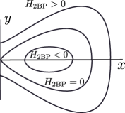
2. The -body Problem
In this section we recall some well known facts about the -body Problem (2BP) which will be used in the following. In polar coordinates, the Hamiltonian of the 2BP reads (compare (1.1))
| (2.1) |
As for (1.1), the rotational symmetry implies that is a conserved quantity, so we look at (2.1) as a one-parameter family of Hamiltonian functions . For each the Hamiltonian is integrable and the motion can be classified in terms of the value of the energy: negative values correspond to elliptic motions, positive energies correspond to hyperbolic motions and for zero energy the motion is parabolic.
It is also straightforward to check that for all
is a fixed point for the flow of (2.1)444To analyze this fixed point properly one should work in McGehee coordinates, which are introduced in Section 3.2.. Moreover, for all the fixed point posses stable and unstable manifolds which coincide along a one dimensional homoclinic manifold . The homoclinic orbit is indeed the parabolic orbit of the 2BP with angular momentum .
Lemma 2.1.
There exist real analytic functions and , defined for all , such that
| (2.2) |
Moroever, for all and
In addition, for any we have
Remark 2.
Proof.
A proof of the first two items can be found in [MP94], where the authors also show that
One can check that for the second equality admits the unique inverse
which for large yields that
Therefore, as
and the conclusion follows. ∎
Define the local stable and unstable manifolds555One can prove that orbits starting at points in (respectively ) are confined in the region for all positive times (respectively in the region for all negative times).
It is a standard fact that are exact Lagrangian submanifolds so they can therefore be parametrized in terms of a generating function.
Lemma 2.2.
There exists , which satisfies
and such that
3. The dynamics close to
In this section we study the dynamics in a neighbourhood of the periodic orbit at infinity defined in (1.3). Despite being degenerate (the linearized vector field vanishes at ) the flow close to the periodic orbit behaves in a similar way to the flow on a neighbourhood of a hyperbolic periodic orbit.
3.1. The local invariant manifolds
Let be the time flow associated with the Hamiltonian defined in (1.2). It is a classical result by McGehee [McG73] (see also [BF04]) that posses local stable and unstable invariant manifolds (by we denote the projection on the and coordinates of a point )
| (3.1) |
It is also a standard fact that are exact Lagrangian submanifolds so they can be parametrized in terms of a generating function. The following result follows directly from the arguments in the proof of Theorem 4.4. in [GPSV21] (see Remark 3).
Proposition 3.1 ([GPSV21]).
Remark 3.
In Theorem 4.4. in [GPSV21] the authors only show the existence of the generating functions for large values of . The reason is that, under the hypothesis of large , they can extend the generating functions to a common domain where they can measure their diference. However, if we are only concerned with the existence and behaviors of the generating functions close to infinity, the problem is already perturbative, and the very same arguments apply to obtain the conlcusion in Proposition 3.1.
Define the global stable and unstable invariant manifolds
| (3.2) |
The analytic dependence of the functions on and will be key to prove that transversal intersections (whenever they exist) between the global stable and unstable invariant manifolds (3.2) are topologically transverse except for (possibly) a finite subset of values of . This is key for the multibump construction. On the other hand, the estimate as will be needed in the proof of certain technical steps in Lemma 5.5 (see Appendix A).
3.2. The parabolic Lambda Lemma
We now analyze the topology of the flow lines close to the periodic orbit . For that, it is convenient to introduce the McGehee transformation in which the equations of motion associated with the Hamiltonian system in (1.2) read
In this variables, the periodic orbit at infinity (1.3) now corresponds to the periodic orbit . Following Moser [Mos01], we now straighten the stable and unstable directions associated with this periodic orbit. To that end, we introduce the change of variables
In these coordinates
| (3.3) |
so it is clear that the local stable and unstable invariant manifolds associated with the periodic orbit , which, by the work of McGehee [McG73] (see also Proposition 3.1) we already know exist, are close (for small ) to and respectively. Let now, for sufficiently small , define the set
and, let and be graph parametrizations of these local invariant manifolds. Introduce new variables on given by
From the invariance equation satisfied by one can deduce their Taylor expansion around . Then, an easy computation, shows that
| (3.4) |
so in coordinates the local stable and unstable manifolds are the sets and respectively. Define now, for the sections (see Figure 3.2)
and the associated Poincaré map , associated with the flow (3.3), whenever is well defined. Lemma 3.2 shows that a parabolic version of the Lambda Lemma holds for the degenerate periodic orbit . In order to build orbits whose final motions are hyperbolic, we also introduce the outer sections
The proof of the following proposition follows plainly from the arguments in Chapter IV of [Mos01], where an analogous result is proved for the Sitnikov problem. See also Theorem 5.4. in [GMPS22].
Lemma 3.2.
Fix any . Then, there exists sufficiently large and sufficiently small such that for any and any the Poincaré map
is well defined. Moreover, for any sufficiently large there exist unique and , which satisfy
for which .
In addition, for any (respectively ), the orbit of (3.4) with initial condition (respectively ) is defined for all forward (respectively backward) times and satisfies
The first item in Lemma 3.2 shows that the iterates of curves which are transversal to the local stable manifold accumulate along the unstable manifold (see also Figure 3.2). The second item ensures that orbits with initial conditions on (respectively ) have forward (respectively backward) hyperbolic final motions. We now translate these results to the original coordinates. To that end we introduce the sections
and the map whenever is well defined. We also define the sections leading to hyperbolic final motions
Lemma 3.3.
Fix any . Then, there exist sufficiently large such that for any there exists such that for all the Poincaré map
is well defined for and some . There exists such that for any there exist unique such that . Moreover, for any there exists such that, if and , then
In addition, the orbit of (1.2) with initial condition (respectively ), is defined for all forward (respectively backward) times and satisfies
4. Existence of homoclinic orbits to
In this section we establish the existence of orbits of the Hamiltonian (1.1), which are homoclinic to . For , the Hamiltonian (1.1) can be considered as a perturbation of the integrable 2BP, in which there exists a homoclinic manifold to (see Lemma 2.1). Therefore, for , one can use geometric perturbation theory to prove that the global invariant manifolds and defined in (3.2) intersect transverally. This was the approach used in [GPSV21] where the following result was proved.
Theorem 4.1 ([GPSV21]).
There exists such that for all such that the global stable and unstable manifolds and defined in (3.2), intersect transversally.
Yet, for a fixed , the Hamiltonian (1.1) is not close to the 2BP. Therefore, geometric perturbation theory cannot help to study the existence of transversal intersections between and . We however exploit the variational formulation of the problem, in which the powerful techniques from nonlinear functional analysis are available.
More concretely, in Section 4.1 we introduce a suitable action functional, defined on a suitable Hilbert space, whose critical points are indeed orbits of (1.1) which are homoclinic to . Then, in Section 4.2 we establish the existence of a critical point of the aforementioned action functional using a minmax argument. The minmax characterization of the critical point obtained is crucial for the construction in Section 6.
4.1. The Variational Formulation
We introduce the vector space of real valued functions
| (4.1) |
In the following, we will write (i.e. is the weak derivative of ). It is easy to chek that
defines an inner product on for which the functional space equiped with this inner product is a Hilbert space. We write
for the induced norm. Notice that for all and all
After the introduction of the functional space it is an easy computation to show that the existence of orbits of (1.2) homoclinic to the periodic orbit at infinity is equivalent to the existence of critical points of the action functional given by
| (4.2) |
where
| (4.3) |
stands for the effective potential
| (4.4) |
and with being the parabolic orbit of the 2BP with angular momentum (see Remark 5).
Remark 4.
is indeed a renormalized Lagrangian, that is, we have substracted the term in the integrand of what would be the “natural” action functional. The reason behind the definition of (4.2) is that the action of a parabolic orbit is infinite. Indeed, the Lagrangian of the 2BP reads
and for a parabolic orbit for .
Remark 5.
It might seem surprising that when defining the renormalized Lagrangian , we let be an independent parameter instead of taking . The reason is that in this way, for a fixed and fixed the function is monotonely decreasing. This will allow us to use a monotonicity trick due to Struwe which is key to obtain uniform bounds for certain (Palais-Smale) sequences for which (see Section 4.2.1 and, in particular, 4.7). On the other hand, the asymptotic behavior of parabolic solutions as becomes independent of the value of the angular momentum (see Lemma 2.1) so the definition of the renormalized Lagrangian makes sense for .
Remark 6.
Throughout the rest of the paper the value will be fixed. Thus, we omit the dependence of all quantities on . Having fixed , we state results for (or full measure subsets of this set). This choice is completely arbitrary: the results proved below are certainly true if we replace by any other bounded subset. However, since we have always the freedom to choose as large as we want it is enough to state results for .
The following observation will play an important role in our construction.
Lemma 4.2.
Let and define the translation operator
Then, for all
We now state a technical lemma which will prove useful in later compactness arguments.
Lemma 4.3.
Let and let be the weighted space with norm given by
Then, is continuously embedded in for and compactly embedded in for .
Proof.
The proof of the continuous embedding for is obtained by the very same argument used in the proof of Proposition 3.2. in [BDFT21] taking into account that for and . We now prove that the embedding for is compact. Take any bounded sequence such that weakly in . In particular pointwise for all . Since, for any and any we have
we obtain that for all
Therefore, a direct application of the dominated convergence theorem shows that
∎
We now show that is continuous and has a continuous differential on a suitable subset .
Lemma 4.4.
Let and be two fixed constants and define
Then, for any we have .
Proof.
Let and make use of the mean value theorem to write
| (4.5) |
where for some . On one hand,
as . On the other hand, since for
and convergence in implies uniform convergence in compact intervals, we have, taking into account the expression of (4.4), that
pointwise as . Moreover, for
so, from the definition of in (4.4), a straightforward computation shows that for
Thus, using again that , we obtain the existence of depending only on and such that for all
Therefore,
and the continuity of the map is implied by Lemma 4.3. The proof that is a continuous map follows from similar arguments. ∎
Lemma 4.5.
Let and be two fixed constants and let be the subset defined in Lemma 4.4. Then, for any for any , is a compact perturbation of the identity. In partiuclar, this implies that for any compact set the set is compact.
Proof.
We write
| (4.6) |
where we have introduced the functional
Thanks to Lemma 4.3 we can take
as an equivalent inner product in . It follows from Lemma 4.4 that for all , and are continuous linear functionals and thanks to Riesz representation theorem, for every there exist unique such that
and . After writing
a tedious but straightforward computation shows that for any
| (4.7) |
what implies that is a compact operator (recall that the embedding of in is compact). The second item in the lemma plainly follows after writing
Indeed, for a sequence whose image under is contained in a compact subset there exists a subsequence (which we do not relabel) for which is convergent in . Then, the proof is finished since being a compact operator and implies that (up to passing to a further subsequence) is also convergent in . ∎
From now on we will omit the subscript in the inner product and norm defined in .
4.2. Existence of critical points of the action functional
In this section we prove the existence of critical points of the action functional defined in (4.2) using a minmax argument. In particular, we will employ a constrained version of the celebrated mountain pass theorem of Ambrosetti and Rabinowitz [AR73]. The first step is to verify that the level sets of have a mountain pass geometry. This is the content of the following proposition.
Proposition 4.6.
Take any constant . Then, for all there exist such that
Moreover, there exists such that if we take , then for any curve joining and there exist a point for which
Proof.
Let so
It follows from Fatou’s lemma that
On the other hand, take . Then, for some finite (and uniform for ) we have
Using that for (this can be deduced from the proof of Lemma 2.1) one can easily check that
The first part of the lemma is proven by taking with large enough and with . In order to prove the second item of the lemma we let be such that
and denote by the value of for which for all such that . Notice that exists because of the convexity of for large values of , which can be checked explicitely from the expression of in (4.4). We now take such that . We claim that so the lemma follows since, by continuity, for all joining and there exist a point for which
We now prove the claim. Lemma 4.2 implies that, withouth lost of generality, we can suppose that the minimum is attained at the interval . We express
where
and
For the first term, after applying the mean value theorem twice, we obtain that
with , and , . Since
we have by the definition of . For the second term we use that and that for all we have so we obtain
for some which depends only on . An analogous computation shows that for the third term we have
for some which depends only on . Therefore
for depending only on and the result follows after enlarging (if necessary) while keeping fixed. ∎
We now have established the existence of the mountain pass geometry for the level sets of the functional . The next natural step would be to apply the classical deformation lemma to obtain a Palais-Smale (PS) sequence for the functional . There are however two difficulties. The first one is that, a priori, a suboptimal path, might contain points for which , at which the functional is not continuous. The second difficulty is that, even if we can guarantee that for all in the region where we carry the deformation argument, without further constraints we are not able to show that the PS sequence obtained is precompact. For that reason, we take large enough and we carry the deformation argument in the region
| (4.8) |
In Lemma 4.11 we show that on a suitable subset , the functional is bounded and coercive, from where we deduce a uniform bound for when . This will be crucial to obtain uniformly bounded PS sequences.
4.2.1. The deformation argument
We now introduce the set of curves
| (4.9) |
and for large enough the candidate to critical value
| (4.10) |
The first step in the deformation argument is to prove that there exists a positive such that for all bounded , we have . To that end we notice that
| (4.11) |
with
| (4.12) |
and apply a monotonicity trick due to Struwe (see [Str88] and [Str00]) to show that for almost every , the functional is bounded if is small enough (see Remark 7). The following version of the monotonicity trick was proved in [Jea99]. We provide the proof for the sake of self completeness.
Lemma 4.7.
There exists a full measure subset such that for all there exists constants and for which if then .
Proof.
Since it follows from expression (4.11) and the definition of in (4.10) that is a monotone decreasing function. Therefore, it is differentiable on a subset whose complement has zero measure. Let , and take such that . Take now , then, by decreasing (if necessary) the value of we can assume that
Then
By the hypothesis on there exists an open neighbourhood around for which
and the lemma is proven. ∎
Boundedness of the functional allows us to obtain an a priori estimate for if is bounded.
Lemma 4.8.
Let be such that . Then, there exists a constant , depending only on such that
Proof.
Suppose there exists such that . Since it holds that and we can assume without loss of generalitiy that for all . Take now and write . Then, by the fundamental theorem of calculus, for any
and Hölder’s inequality implies
∎
Remark 7.
In Lemma 5.1, we show that for all , we have for orbits of (1.2) which are homoclinic to . However, that argument does not allow us to conclude that there exist such that for all bounded we have . Therefore, is not clear how to incorporate the a priori estimate in Lemma 5.1 to obtain a minmax critical point.
Assume now that is such that . Therefore, thanks to Lemmas 4.7 and 4.8 it is possible to obtain an inequality of the form
| (4.13) |
for some . Thus, if we moreover assume that and that happens for we can obtain a uniform bound for the norm of . In general, in problems in which the action functional is invariant under integer time translations, the latter assumption introduces no loss of generality and this argument can be employed to obtain uniformly bounded PS sequences.
However, in the present problem, the translation operator , for which we have , is not an isometry in . This introduces certain technicalities in the deformation argument. In order to overcome this technical annoyance we introduce the following definition.
Definition 4.9.
Given we define its barycenter as the functional given by
The following properties of the barycenter functional will be crucial for the deformation argument.
Lemma 4.10.
Proof.
The proof of the first part is a trivial computation. For the second one we express
with
First we notice that there exists such that for all we have and . Indeed, for all
so there exists , depending only on , such that
for all . Therefore, for depending only on ,
The uniform bound from below for follows since there exists and , depending only on , such that
for all . Take now and write
Let . Then for we can write
On one hand for all
and it follows that
The same computation shows that there exists such that
and the lemma is proven. ∎
Together, Lemma 4.7 and Lemma 4.10 imply the following result, which is key in our constrained deformation argument.
Lemma 4.11.
Proof.
Let
We claim that under the hypothesis of the lemma there exists such that
Suppose not, then, by continuity, there exist and sequences , such that in , and
By invariance of the action functional under translation (see Lemma 4.2) and the fact that
the sequence , satisfies
However, the first two properties imply the existence of such for all . Indeed, by the construction of , for all we have
Moreover, since and , Lemma 4.7 implies that there exists such that for all . Therefore, it is easy to check that there exists such that
for all . Thus, since and is bounded, the sequence must be uniformly bounded. It is easy to check that the existence of such that is in contradition with being unbounded.
Once we know that the claim holds, we obtain that for all . Therefore, since , we have that
for some depending only on and . The result follows since now we can show that for all we have
for some uniform on . ∎
In Proposition 4.13 we show the existence of a PS sequence contained in for large enough values of and . Notice that in particular, thanks to Lemma 4.11 this sequence will be uniformly bounded.
We split the proof of Proposition 4.13 in two parts. First, we assume by contradiction that there exists no critical point of the action functional in . Under this assumption, we build a pseudo gradient vector field for , this is the content of Proposition 4.12. Then, in Proposition 4.13 we use this pseudo gradient vector field to build a localized deformation which yields points for which , a contradiction.
Before stating Proposition 4.12 some definitions are in order. Let and where is the constant in Lemma 4.7. For we want the flow along the pseudogradient vector field to leave positively invariant, we express it as the convex combination of two localized vector fields: a gradient-like vector field supported on
| (4.15) |
and a vector field supported on
| (4.16) |
for which is positively invariant. This construction is made explicit in the following proposition.
Proposition 4.12.
Let be the subset obtained in Lemma 4.7. Let be the constant in Lemma 4.7 and take large enough. Assume that for all there exists for which
Then, there exists such that for all there exists a Lipschitz pseudogradient vector field such that
-
•
,
-
•
There exists a constant such that
-
•
The region is positively invariant under the flow of .
Proof.
Let , define the sets
and the function
which satisfies on and on . We also introduce
and define the function
which satisfies on and on . Take now a sufficiently small open neighbourhood , . Notice that by Lemma 4.11, there exists such that
Then, since , Lemmas 4.7 and 4.8, impy that there exists such that
Therefore, by Lemma 4.4 we have that , what implies the existence of a constant such that . We introduce now the pseudogradient vector field
| (4.17) |
where is the constant vector field given by the constant . Notice that for a large enough fixed , and for all there exists such that
| (4.18) |
Indeed
and the claim follows since for large enough the integrand is non positive and moreover it is strictly negative on a positive measure subset of the real line since (thanks to Lemma 4.11) there exists such that . It is straightforward to chek that the pseudogradient vector field introduced in (4.17) satisfies the properties listed in the statement in the lemma with .
∎
Proposition 4.13.
Proof.
Let be the set defined in (4.9). Let and take a suboptimal path for which for all such that . For all we define the set
Notice that for each , the set is a compact subset of . Denote by
and consider the translated path for . It satisfies that
Let be the pseudogradient vector field built in Proposition 4.12 and denote by its time flow. Notice that since is Lipschitz the flow is well defined at least for sufficiently small . Let be the constant in Proposition 4.12. We claim that the deformed path with satisfies
To verify the claim we first notice that the maximal displacement is bounded by
Therefore, applying Lemma 4.10, we obtain that for any (taking sufficiently large)
Thus, since the region is forward invariant by the flow and
in order to verify the claim, it is enough to check that there does not exist
for which where is the set defined in (4.15). This is clearly not possible since for we have
so
a contradiction. Now that the claim is verified consider the path
It satisfies that
and
If the proposition is proved. In the case we repeat the argument above with the path to obtain a path satisfying
and
The result follows after repeating the construction no more than steps. ∎
Finally, we obtain the existence of a critical point of the functional at a level .
Theorem 4.14.
Let be the subset obtained in Lemma 4.7. Then, for all there exists a critical point of the action functional at the level .
5. Topological transversality between the stable and unstable manifolds
For the choice of was arbitrary, Theorem 4.14 implies that for any compact subset of the real line, there exists a full measure subset such that for all there exists an orbit of (1.1) which is homoclinic to . Another way of rephrasing Theorem 4.14 is that the invariant manifolds manifolds defined in (3.2) intersect for almost all values of in . However, Theorem 4.14 contains no information about the geometry of the intersection, in particular wether it is transversal or not.
Theorem 4.1, proved in [GPSV21], shows that the intersection between is transverse for all sufficiently large. Moreover, the local stable manifolds (see (3.1)) depend analytically on and (see Proposition 3.1). We want to exploit this facts to deduce that the intersection of the manifolds (which, by Theorem 4.14 we already know that exists for almost all values of ) must be topologically transverse for almost all values of in .
Remark 8.
In the following we fix a sufficiently large value of and work with .
The first step is to obtain an a priori estimate from below for .
Lemma 5.1.
Let and let be an orbit of of the Hamiltonian in (1.1) which is homoclinic to . Then, for all we have
Proof.
Since is an orbit of of the Hamiltonian we have that
| (5.1) |
Let now be an interval in which for all . Then, multiplying (5.1) by , for all we obtain
that is, the energy
is non increasing on the interval . Let be a maximal interval in which is decreasing: we distinguish between two alternatives, either
-
•
, and , and , or
-
•
and , and
for some . In the first case we have
In the second case, using that , and the inequality (5.1), we obtain
Therefore, in both cases, for all we have , which implies that
∎
Lemma 5.1 implies that for , homoclinic orbits do not intersect the section . This fact allows us to exploit the analytic dependence of the Hamiltonian in the parameter to prove the following result.
Lemma 5.2.
The set of values of for which , is finite.
Proof.
Fix any and let be the constant in Theorem 4.1 and let be such that for all the generating function associated with the local stable manifold (see 3.1) is well defined for all . Define the set
Whenever it exists, denote by the connected component of associated with the first backwards intersection of with (see Figure 5.1). Define now the set
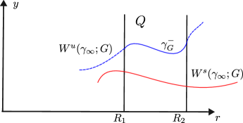
Clearly, where
In view of Lemma 5.1, for all
| (5.2) |
so is a closed set. Moreover, since the Hamiltonian (1.2) depends analytically on , and, by (5.2), for all the vector field associated with (1.2) is analytic on a neighbourhood of , there exists an open subset such that and in which . Define now the function given by
which satisfies for all and . Suppose now that . Then, for all and we obtain a contradiction with the fact that for the manifolds , intersect transversally (see Theorem 4.1). Therefore, . We now show that, moreover, cannot contain any accumulation point. To see this suppose that there exists such that
Since there exists an open interval such that . Then, the fact that implies that and since is an acuumulation point of we conclude that on . Then , so there exists such that , a contradiction with the definition of . ∎
Lemma 5.3.
For all the set is isolated in .
Proof.
Following [MNT99], we define the map given by
We now show that the set is isolated in . Suppose on the contrary that there exists an accumulation point , then, there exist and such that , and
Thus, there exist infinitely many different homoclinic points contained in the piece of the local stable manifold for any . This would imply the existence of , such that intersect at infinitely many points, where .However, and are compact analytic curves, and since they cannot intersect at infinitely many points.
By Lemma 3.3. in [MNT99], the function is continuous, so the lemma is proven, for if it were to be false there would exist an accumulation point . ∎
The fact that the critical points are isolated implies the following non-degeneracy property at, at least, one of the critical points of at the level . We say that has a local mountain pass structure if, for all neighbourhood of , the set is not path connected. The following result is a direct consequence of Lemma 5.3 and Theorem 1 in [Hof86].
Proposition 5.4.
For all there exists such that which has a local mountain pass structure.
Remark 9.
In all the forthcoming sections we fix where is the set defined in (5.3) and omit the dependence on .
5.1. The reduced action functional
For we denote by the usual Sobolev space consisting of functions defined on the interval with one weak derivative in and introduce the restriction operator
| (5.4) | ||||
Then, for a sufficiently small neighbourhood of a point where and a sufficiently large (depending on ) we define the reduced action functional given by
where the renormalized Lagrangian is defined in (4.3) and are the generating functions of the local stable and unstable manifolds which were obtained in Proposition 3.1. Notice that for sufficiently large (depending on ) and sufficiently close to the values are contained in .
We now want to translate the results we have obtained for the functional , in particular Proposition 5.4, in results for the functional . To that end, given any constant and we introduce the functional spaces
and
Define also the weakly closed subsets
Then, we define the asymptotic actions
| (5.5) |
Lemma 5.5.
For all there exists such that for all there exists a unique such that
Moreover,
Proof.
A simple computation shows that
from where we easily deduce that there exists such that, if
then, the functional in (5.5) is strictly convex on the strictly convex set . Therefore, there exists a unique minimizer for which
Moreover, is easy to check that is a critical point of the functional . Consequently, is an orbit of (1.1) asymptotic in the future to .
Let now be the generating function of the local stable manifold introduced in Proposition 3.1. By uniqueness of the local stable manifold, the function satisfies that
for all . In particular, since moreover Lemma A.2 in Appendix A implies that as and since as , we can integrate by parts to obtain
On the other hand,
where we have used that and the fact that
which is also proved in Lemma A.2. ∎
Introduce now the extension operator
| (5.6) |
where
From the proof of Lemma 5.5 we deduce the following.
Lemma 5.6.
Let , let sufficiently large, let and let a sufficiently small neighbourhood of . Then, the extension operator (5.6) is well defined on .
The proof of the following Lemma is an straightforward consequence of the definition of the extension operator .
Lemma 5.7.
Let . Then, for sufficiently large and all contained in a sufficiently small neigubourhood of
Also, for all in a sufficiently small neighbourhood of
Moreover, for such that we have .
We can now translate the result for stated in Proposition 5.3 in an analogous result for .
Proposition 5.8.
There exists and which is a critical point of and has a local mountain pass structure.
Proof.
The proof is a simple combination of the proof of Theorem 1 in [Hof86] together with the relationship between the functionals and which was obtained in Lemma 5.7. We sketch here the details for the sake of completeness.
Denote by where is the critical value defined in (4.10). Lemma 5.3 implies, in particular, that is an isolated subset in . Moreover, fixing sufficiently large where was defined in (4.8). Let now and be a suboptimal path at level . Then, intersects a finite number of elements in , which we denote by for some finite . Let now sufficiently small and denote by the ball of radius around . Without loss of generality we can assume that intersects each only once so we can define (see Figure 5.2)

and and . Let now large enough and small enough so the restricition operator in(5.4) is well defined on . Let . Again, without loss of generality, we can assume that for all , have minimizing tails, that is, is the unique minimizer of on and is the unique minimizer of on . Now, define the paths
for , and the points , which are indeed critical points of the reduced action functional . Suppose the point does not have a local mountain pass structure. Then, we can build (see Lemma 1 in [Hof86]) a continuous deformation such that
where by we denote the closure of the ball . Write , which satisfies
and
Now, for the extension operator is well defined on (shrinking if necessary) and , we can define the path which, by construction, satisfies
and
The proposition is therefore proved for, if none of the points posses a local mountain pass structure, the continuous path defined by gluing (in the obvious way) the segments with the segments satisfies , a contradiction. ∎
Proposition 5.8 entails a non degeneracy condition for the intersection of the invariant manifolds and at the homoclinic orbit associated with . We now make use of topological degree theory to exploit this non degeneracy condition. Let be the critical point obtained in Proposition 5.8 and consider a sufficiently small neighbourhood such that . By definition of the functional , and the fact that
the differential is a continuous linear functional and, for any and any , we can express
| (5.7) |
where we have introduced the functional (compare expression (4.6) in the proof of Lemma 4.5)
Since and the interval is compact, the expression
defines an equivalent inner product on . For , denote by the unique element of such that for all
| (5.8) |
From (5.7) one easily deduces that the map is a compact perturbation of the identity. Therefore, for any subset and any point such that the Leray-Schauder degree 666The Leray-Schauder degree is a generalization of the Brouwer degree to maps between infinite dimensional spaces wich are of the form identity+compact. Details about its definition and properties can be found in [Kie12]. associated with the triple , which we denote by
is well defined. Proposition 5.8, together with Theorem 2 in [Hof86], imply the following result.
Proposition 5.9.
Let be the critical point of which was obtained in Proposition 5.8 and, for , denote by the ball of radius centered at . Then, there exists such that for all ,
As a consequence of Proposition 5.9 we can prove that the manifolds and intersect transversally for . First, we introduce some notation which will be useful in the proof of Proposition 5.10 and in Section 6. Let , then, we denote by the evaluation operator given by
In addition we denote by the unique element such that for all
Proposition 5.10.
For all there exists a topologically transverse intersection between and .
Proof.
Let be the critical point obtained in Proposition 5.8. Then, there exists such that for all
In particular, there exists such that
Define now, for , the one parameter family of maps given by
Then, it is possible to find such that is an admissible homotopy for so by invariance of the degree under admissible homotopies
We now show how this implies the desired conclusion. Let . Then, denoting by the projections onto the coordinates of a point , and by the flow at time associated to Hamiltonian (1.2) we have that
for . This completes the proof. ∎
6. Construction of multibump solutions
We now show how Proposition 5.9 together with the parabolic lambda Lemma 3.2 can be used to the deduce the existence of homoclinic orbits to which perform any arbitrary number of “bumps”. We start by stating the following lemma, which is nothing but a reformulation of the parabolic lambda Lemma 3.3.
Lemma 6.1.
There exists large enough such that for there exists such that for all there exists a unique orbit of (1.1) for which and . Moreover, for all there exists such that for all the unique solution satisfies
6.1. Proof of Theorem 1.5
We are now ready to build the multibump solutions. By proposition 5.9 we know that there exists a critical point of and such that for all ,
where stands for the ball of radius centered at . For any , introduce now the map
| (6.1) | ||||
where the maps , are given by
and for (this set is empty for )
The proof of the following result follows inmediately after from Proposition 5.9 and Lemma 6.1.
Theorem 6.2.
There exists , and such that for all
In particular, for any sequence there exists such that
Theorem 6.2 shows the truth of the first item in Theorem 1.5 for sequences with finite, but arbitrarily large number of nonzero entries. For the time interval in the definition of (6.1) does not depend on , the existence of solutions such that has infinitely many non-zero entries follows by a standard diagonal argument in the topology. In order to deduce the second item, namely the existence of infinitely many periodic orbits, we define the functional
| (6.2) | ||||
with periodic boundary conditions
and such that for (this set is empty for ) has the same expression as in in the non periodic case. The proof of Theorem 1.5 is complete.
6.2. Proof of Theorem 1.4
From the proof of Theorem 1.5 it follows that
for any possible combination of and . We now show that (the proof for the other combinations being similar). The following result is implied by the second part of Lemma 3.3.
Lemma 6.3.
There exists large enough and such that for all and all there exists a unique orbit of (1.1) for which
Moreover, is defined for all and satisfies
Given and we denote by
where is the orbit segment found in Lemma 6.3. Fix . The fact that follows from the fact that the functional
where the maps , are given by
and for (this set is empty for )
In order to prove that we take and argue as in the proof of Theorem 1.5. In order to show that we impose periodic boundary conditions. The proof of Theorem 1.4 is complete.
Appendix A Proof of of the technical claims in Lemma 5.5
We first prove the following result, which will be needed for the proof of Lemma A.2.
Lemma A.1.
Let be the generating function defined in Lemma 2.2. Then, for any we have that
Proof.
Denote by the unique function such that, for all , the component of the parametrization (2.2) is given by . Writing we observe that satisfies
Using now that for large we obtain that
so
as was to be shown. ∎
The claims in Lemma 5.5 follow from the following result.
Lemma A.2.
Suppose that for there exists an orbit of the Hamiltonian in(1.2) which is homoclinic to and, for some satisfies
Then,
and, in particular
Proof.
We write
On one hand, it follows from the last item in Lemma 3.1 that as
On the other hand, it follows from the mean value theorem, the definition of and the hypothesis in the statement of the lemma that as
for . Also, from Lemma 2.2 we deduce that
The proof of the first item follows combining the estimates for and integrating. The second part follows from the obtained estimate and straightforward computations. ∎
References
- [Ale69] V. M. Alekseev. Quasirandom dynamical systems. mat. Zametki, 6:489–498, 1969.
- [AR73] Antonio Ambrosetti and Paul H. Rabinowitz. Dual variational methods in critical point theory and applications. J. Functional Analysis, 14:349–381, 1973.
- [BDFT21] Alberto Boscaggin, Walter Dambrosio, Guglielmo Feltrin, and Susanna Terracini. Parabolic orbits in celestial mechanics: a functional-analytic approach. Proc. Lond. Math. Soc. (3), 123(2):203–230, 2021.
- [BF04] I. Baldomá and E. Fontich. Stable manifolds associated to fixed points with linear part equal to identity. J. Differential Equations, 197(1):45–72, 2004.
- [CGM+21] Maciej J Capiński, Marcel Guardia, Pau Martín, Tere Seara, and Piotr Zgliczyński. Oscillatory motions and parabolic manifolds at infinity in the planar circular restricted three body problem. arXiv preprint arXiv:2106.06254, 2021.
- [Cha22] Jean Chazy. Sur l’allure du mouvement dans le problème des trois corps quand le temps croît indéfiniment. Ann. Sci. École Norm. Sup. (3), 39:29–130, 1922.
- [CZES90] Vittorio Coti Zelati, Ivar Ekeland, and Éric Séré. A variational approach to homoclinic orbits in Hamiltonian systems. Math. Ann., 288(1):133–160, 1990.
- [CZR91] Vittorio Coti Zelati and Paul H. Rabinowitz. Homoclinic orbits for second order Hamiltonian systems possessing superquadratic potentials. J. Amer. Math. Soc., 4(4):693–727, 1991.
- [GK11] Joseph Galante and Vadim Kaloshin. Destruction of invariant curves in the restricted circular planar three-body problem by using comparison of action. Duke Math. J., 159(2):275–327, 2011.
- [GK12] A. Gorodetski and V Kaloshin. Hausdorff dimension of oscillatory motions for restricted three body problems. Preprint, available at http://www.terpconnect.umd.edu/ vkaloshi, 2012.
- [GMPS22] Marcel Guardia, Pau Martín, Jaime Paradela, and Tere M. Seara. Hyperbolic dynamics and oscillatory motions in the 3 body problem, 2022.
- [GMS16] Marcel Guardia, Pau Martín, and Tere M. Seara. Oscillatory motions for the restricted planar circular three body problem. Invent. Math., 203(2):417–492, 2016.
- [GPSV21] Marcel Guardia, Jaime Paradela, Tere M Seara, and Claudio Vidal. Symbolic dynamics in the restricted elliptic isosceles three body problem. Journal of Differential Equations, 294:143–177, 2021.
- [GSMS17] Marcel Guardia, Tere M. Seara, Pau Martín, and Lara Sabbagh. Oscillatory orbits in the restricted elliptic planar three body problem. Discrete Contin. Dyn. Syst., 37(1):229–256, 2017.
- [Hof86] Helmut Hofer. The topological degree at a critical point of mountain-pass type. In Nonlinear functional analysis and its applications, Part 1 (Berkeley, Calif., 1983), volume 45 of Proc. Sympos. Pure Math., pages 501–509. Amer. Math. Soc., Providence, RI, 1986.
- [Jea99] Louis Jeanjean. On the existence of bounded Palais-Smale sequences and application to a Landesman-Lazer-type problem set on . Proc. Roy. Soc. Edinburgh Sect. A, 129(4):787–809, 1999.
- [Kie12] Hansjörg Kielhöfer. Bifurcation theory, volume 156 of Applied Mathematical Sciences. Springer, New York, second edition, 2012. An introduction with applications to partial differential equations.
- [Koz83] V. V. Kozlov. Integrability and nonintegrability in Hamiltonian mechanics. Uspekhi Mat. Nauk, 38(1(229)):3–67, 240, 1983.
- [LS80a] Jaume Llibre and Carles Simó. Oscillatory solutions in the planar restricted three-body problem. Mathematische Annalen, 248(2):153–184, 1980.
- [LS80b] Jaume Llibre and Carlos Simó. Some homoclinic phenomena in the three-body problem. J. Differential Equations, 37(3):444–465, 1980.
- [McG73] Richard McGehee. A stable manifold theorem for degenerate fixed points with applications to celestial mechanics. J. Differential Equations, 14:70–88, 1973.
- [MNT99] Piero Montecchiari, Margherita Nolasco, and Susanna Terracini. A global condition for periodic Duffing-like equations. Trans. Amer. Math. Soc., 351(9):3713–3724, 1999.
- [Moe07] R. Moeckel. Symbolic dynamics in the planar three-body problem. Regul. Chaotic Dyn., 12(5):449–475, 2007.
- [Mos01] Jürgen Moser. Stable and random motions in dynamical systems. Princeton Landmarks in Mathematics. Princeton University Press, Princeton, NJ, 2001. With special emphasis on celestial mechanics, Reprint of the 1973 original, With a foreword by Philip J. Holmes.
- [MP94] Regina Martínez and Conxita Pinyol. Parabolic orbits in the elliptic restricted three body problem. J. Differential Equations, 111(2):299–339, 1994.
- [MV09] E. Maderna and A. Venturelli. Globally minimizing parabolic motions in the Newtonian -body problem. Arch. Ration. Mech. Anal., 194(1):283–313, 2009.
- [MV20] Ezequiel Maderna and Andrea Venturelli. Viscosity solutions and hyperbolic motions: a new PDE method for the -body problem. Ann. Math. (2), 192(2):499–550, 2020.
- [Sér92] Eric Séré. Existence of infinitely many homoclinic orbits in Hamiltonian systems. Math. Z., 209(1):27–42, 1992.
- [Str88] Michael Struwe. The existence of surfaces of constant mean curvature with free boundaries. Acta Math., 160(1-2):19–64, 1988.
- [Str00] Michael Struwe. Variational methods, volume 34 of Ergebnisse der Mathematik und ihrer Grenzgebiete. 3. Folge. A Series of Modern Surveys in Mathematics [Results in Mathematics and Related Areas. 3rd Series. A Series of Modern Surveys in Mathematics]. Springer-Verlag, Berlin, third edition, 2000. Applications to nonlinear partial differential equations and Hamiltonian systems.
- [SZ20] Tere M. Seara and Jianlu Zhang. Oscillatory orbits in the restricted planar four body problem. Nonlinearity, 33(12):6985–7015, 2020.
- [Xia94] Zhihong Xia. Arnold diffusion and oscillatory solutions in the planar three-body problem. J. Differential Equations, 110(2):289–321, 1994.