Oscillator strengths and excited-state couplings for double excitations in time-dependent density functional theory
Abstract
Although useful to extract excitation energies of states of double-excitation character in time-dependent density functional theory that are missing in the adiabatic approximation, the frequency-dependent kernel derived earlier [J. Chem. Phys. 120, 5932 (2004)] was not designed to yield oscillator strengths. These are required to fully determine linear absorption spectra and they also impact excited-to-excited-state couplings that appear in dynamics simulations and other quadratic response properties. Here we derive a modified non-adiabatic kernel that yields both accurate excitation energies and oscillator strengths for these states. We demonstrate its performance on a model two-electron system, the Be atom, and on excited-state transition dipoles in the LiH molecule at stretched bond-lengths, in all cases producing significant improvements over the traditional approximations.
The challenge of describing excited states of double-excitation character has grown from being a relatively minor nuisance in certain regions of linear response spectra to being a real hindrance in our ability to simulate photo-excited dynamics in molecules. These states are loosely defined in the sense of having a significant proportion of doubly-excited determinants with respect to a reference ground-state Slater determinant, where a doubly-excited determinant promotes two occupied orbitals of the reference determinant to two virtual ones Maitra (2022).
In ground-state spectra these states have typically smaller transition strengths (“darker") than predominantly singly-excited states but they can siphon off oscillator strength of neighbouring single-excitations whose absorption peaks will be overestimated in simulations that do not account for double-excitations. Moreover, these states are readily accessible when a molecule is excited, offering photochemical/physical pathways that play a role in a range of applications, from photocatalytic design, photo-induced charge transport, to laser-driven or polariton-enabled control. While the true correlated excited-state wavefunctions contain contributions from double excitations, these are either absent in approximate electronic structure methods or poorly approximated, resulting in states missing from the spectrum, or with energies and transition strengths with larger errors than for states with predominantly single-excitation character Loos et al. (2019), wreaking havoc on predictions of excited-state dynamics.
The problem is particularly severe for single-reference methods in their usual modus operandi, such as time-dependent density functional theory (TDDFT) within the adiabatic approximation Jamorski, Casida, and Salahub (1996); Tozer and Handy (2000); Maitra et al. (2004); Maitra (2022), equation-of-motion coupled-cluster (EOM-CC) with singles and doubles only Hirata, Nooijen, and Bartlett (2000); Loos et al. (2019), or the Bethe-Salpeter equation with the GW approximation (GW-BSE) with static screening Romaniello et al. (2009); Sangalli et al. (2011); Bintrim and Berkelbach (2022). While double-excitation character can be adequately included in EOM-CC if triple excitations are included in the cluster expansion, and in GW-BSE with full frequency-dependence or equivalently in an expanded excitation space, these procedures increase the computational cost of these methods, both of which are already more expensive than TDDFT. Multiconfigurational methods may be better platforms for these states, but aside from their higher computational cost, other issues enter such as gauge-sensitivity, and the sizes of an adequate active space which can change during a dynamical process. For determination of oscillator strengths for these states (or any excited state) the difficulty increases significantly since increased accuracy requires cranking up the number of electronic configurations more so than for corresponding improvement in energies, which results in a large increase in the computational costDamour et al. (2023); Sarkar et al. (2021).
Fixing adiabatic TDDFT thus becomes an attractive option. Indeed, double-excitations provide a prime example where TDDFT in theory and in practise diverge: in theory, their excitation energies and oscillator strengths are captured exactly, but the approximate functionals used in practise cannot capture them. It is now well-known that the culprit is the adiabatic nature of the approximation Jamorski, Casida, and Salahub (1996); Tozer and Handy (2000); Maitra et al. (2004); Maitra (2022): the exact exchange-correlation (xc) kernel has a strong frequency-dependence (a pole) that effectively folds a double-excitation of the non-interacting Kohn-Sham (KS) system into the TDDFT response equations, but adiabatic approximations use a frequency-independent kernel. The frequency-dependence implicit in orbital-dependence of a hybrid functional does not have the correct structure. Using first-principles arguments, Ref. Maitra et al. (2004) proposed a frequency-dependent kernel, sometimes called “dressed TDDFT", that has been shown to successfully capture the energies of double-excitations in a range of molecules Cave et al. (2004); Elliott et al. (2011); Huix-Rotllant et al. (2011); Mazur and Włodarczyk (2009); Mazur et al. (2011). However, it is unable to yield information on the oscillator strengths because it is designed to operate within the framework of a Tamm-Dancoff-like approximation which does not preserve oscillator strengths.
In this Communication, we derive a kernel designed to work within full TDDFT linear response, which yields both excitation energies and oscillator strengths of these states, preserving the oscillator strength sum-rule. We demonstrate its accuracy on a two-electron model system, the lowest excitations in the Be atom, and the LiH molecule over a range of interatomic separations. The kernel provides an approximation of how the transition density of a KS single excitation gets distributed into mixed single- and double-excitations of the true system. This enters into a formula to compute excited-to-excited state transition densities that was recently derived Dar, Roy, and Maitra (2023) to tame unphysical divergences in the adiabatic quadratic response function giving an improvement in the transition dipole between two states in the LiH molecule as it begins to dissociate, with accuracy similar to that of the more ad hoc pseudowavefunction approximation Li and Liu (2014); Zhang and Herbert (2015); Ou, Alguire, and Subotnik (2015); Ou et al. (2015); Parker, Roy, and Furche (2016).
In TDDFT, excitation spectra are extracted from the linear response of the density, usually cast in the form of a matrix equation in the space of single KS excitations, , with labelling occupied (unoccupied) orbitals Casida (1995); Petersilka, Gossmann, and Gross (1996); Grabo, Petersilka, and Gross (2000); Gross and Maitra (2012):
| (1) |
where
| (2) |
Here is the matrix element of the Hartree-exchange-correlation kernel, with , being the product of occupied and unoccupied orbitals. The KS frequencies are corrected to the true ones through solving Eq. (1). While the square-root of the (pseudo-)eigenvalues, , give the excitation frequencies of the physical system, the oscillator strength of the transition can be obtained from when normalized according to Casida (1995)
| (3) |
Oscillator strengths (or any one-body transition properties) can be obtained from these eigenvectors, through
| (4) |
where on the right with being a vector in single-excitation space with matrix elements and is a diagonal matrix . The oscillator strength sum-rule, is satisfied by both the true and KS systems and Eq. (4) gives the contributions of the KS oscillator strengths to a given true through the normalized eigenvector . In the adiabatic approximation has no frequency-dependence so the (pseudo-)eigenvectors are just normalized to , but a frequency-dependent kernel causes a redistribution of oscillator strengths through Eq. (3).
A key point is that, whether with a frequency-dependent kernel or not, accurate oscillator strengths fulfilling the oscillator strength sum-rule can only be obtained when the full TDDFT matrix Eq. (2) is used, i.e. including both backward and forward transitions Gross and Maitra (2012); Hirata and Head-Gordon (1999). Backward transitions are neglected in the Tamm-Dancoff approximation where eigenvalues of the corresponding matrix are directly the frequencies (rather than ). Although this approximation has been argued to sometimes give more accurate excitation energies with some approximate functionals Liang et al. (2022); Casida et al. (2000); Hirata and Head-Gordon (1999), the oscillator strengths are generally worse, and the sum-rule violated.
Eq. (3), derived in Ref. Casida (1995), does not appear to be well known and, to our knowledge, used only once before Carrascal et al. (2018) in a detailed study of the linear response of the Hubbard dimer. In general, there has been much more attention paid to excitation energies than to oscillator strengths and the latter have only been studied with the adiabatic approximation Sarkar et al. (2021); Chrayteh et al. (2021); Robinson (2018); Caricato et al. (2011); Laurent and Jacquemin (2013) with eigenvectors normalized to 1. Most interesting for present purposes, Eq. (3) tells us how the oscillator strength of a KS single excitation that lies near a KS double excitation shatters into oscillator strengths of the mixed single and double excitations, when an appropriate frequency-dependent kernel is used.
Consider the limit that a KS excitation is isolated enough in energy from neighbouring excitations, such that the diagonal corrections in the TDDFT matrix dominates, and the full TDDFT matrix Eq. (2) locally reduces to the “small-matrix approximation (SMA)",
| (5) |
Setting this equal to , we observe that frequency-dependence of the kernel creates more than one TDDFT excitation from this single KS excitation. The eigenvectors reduce to one number for each eigenvalue, and indicate the fraction of the KS oscillator strength that goes into the corresponding true transition, with the second equality in Eq. (4) reducing to
| (6) |
In this case, the oscillator strength associated with this isolated KS transition will be preserved over the true excitations in this subspace provided that the approximation for that will go into gives eigenvectors with the property :
| (7) |
where labels the excitations generated from the single KS excitation by the frequency-dependent kernel. This is an important condition for the approximation for . We note that it is satisfied for any of the form
| (8) |
where are constants.
We further note that since the matrix elements in Eq. 4 (Eq. 6) involve a one-body operator, then in the limit that the true ground-state is dominated by a single Slater determinant (weak interaction limit), only the underlying single-excitation components of contribute to . Since , this means that contains the double-excitation (and any higher-excitation) contribution, in this limit.
While the “dressed TDDFT" kernel derived in Ref. Maitra et al. (2004) has the correct form of frequency-dependence to yield energies of double-excitations, it is based on the Tamm-Dancoff approximation, which reduces to the single-pole approximation (SPA) in the isolated KS excitation case, and cannot be used in a consistent way to obtain oscillator strengths. Instead, here we follow a similar approach to Ref. Maitra et al. (2004) but within the SMA. We begin by writing the many-body time-independent Schrödinger equation such that square of the frequency is the eigenvalue: , evaluating this eigenvalue problem in the KS basis, and working in the limit where a KS single-excitation and double-excitation are well-separated in energy from all the other excitations of the system. We define as the sum of the KS single-excitations and such that is close to . Diagonalization then yields
| (9) |
where are the matrix elements of the interacting Hamiltonian in the basis which spans the truncated Hilbert space containing the single and the double excitations, and is the ground state energy. However Eq. (9) is nothing but exact diagonalization in the KS basis; to take advantage of the correlation contained in ground-state TDDFT approximations and to extract a frequency-dependent kernel for an improved TDDFT approximation, we replace with its adiabatic SMA value, and identify the remainder as defining a frequency-dependent kernel:
| (10) | |||||
| (11) |
In Eq. (11) we also replaced in Eq. (9) by to better balance errors in the truncated matrix elements (as was done for the dressed SPA of Ref. Maitra et al. (2004)).
Eq. (11) is our central equation, and it becomes exact in the limit that the coupling between the single and double excitation induced by the electron-interaction is much stronger than the coupling with other single excitations. While the adiabatic approximation merely shifts the KS frequency, Eq. (11) creates a new one, yielding two positive frequencies which approximate the mixed single- and double- excitations of the true system, similar to the dressed SPA kernel of Ref. Maitra et al. (2004). However, unlike that kernel, Eq.(11) preserves the oscillator strength:
It has the form of Eq. 8 and using Eq. (5) with Eq. (11), Eq. (3) explicitly finds that the eigenvectors (one number for each eigenvalue in this case) are such that , thus satisfying the sum-rule (Eq. 7),
| (12) |
The resulting from Eq. (3) gives the fraction of the KS oscillator strength that goes into the respective transition (see Eq. (6)), with giving the double (and higher) excitation contribution to that state in the limit that the ground-state is dominated by a single determinant (see earlier).
In the limit that the coupling between the single and double excitation goes to zero, Eq. 11 correctly reduces to the adiabatic approximation chosen for . When is much smaller than all the other terms, then one frequency is a slightly corrected adiabatic value, while the other reduces to . This motivates a variation of Eq. (11) where we replace the diagonal matrix element differences with KS values:
| (13) |
Another possibility is to replace them with their adiabatic TDDFT counterparts:
| (14) |
where are the adiabatic TDDFT frequencies that correct the bare KS frequencies . Eq. (13) and (14) have a numerical advantage in requiring less two-electron integrals than in Eq. (11) but all three flavours of DSMA capture excitation energies and oscillator strengths of double excitations as we will now demonstrate on explicit examples.
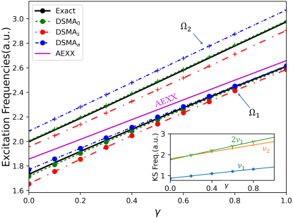
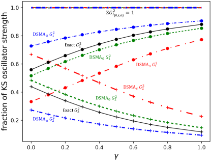
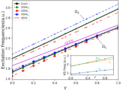
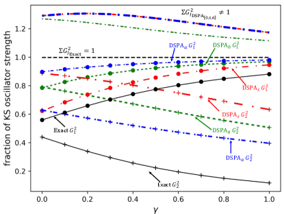
Figure 1 shows the performance on an exactly-solvable model system: two electrons in a one-dimensional harmonic plus linear potential, where is a parameter in the range; varying tunes the degree of mixing of the single and double-excitation character in the interacting excited states. The electrons interact via a soft-Coulomb interaction: . We observe in Fig. 1(a) that for small enough the exact KS system has a double excitation lying very close to the second KS single excitation, with which it mixes strongly when the interaction is turned on as in the physical system, producing two states. As expected, the adiabatic approximation, here chosen to be exact exchange (AEXX), is blind to the double excitation and has only one excitation in this region of the spectrum, while all DSMA approximations correctly yield two excitations. (Note that the exact ground-state KS potential is used to find the bare KS orbitals and energies, while AEXX is used for ). Out of the DSMA’s outlined above, DSMA0 performs the best, giving excitation frequencies very close to the exact. The excitation energies provided by each variant of DSMA are close to those given by the corresponding version of DSPA (see the Supplementary Material). However, the real and significant improvement of DSMA over DSPA lies in its capacity to accurately determine oscillator strengths. Fig. 1(b) shows the fractions of oscillator strength shared by the two states. Again we see that DSMA0 is closest to the exact, but all give a significant improvement over the adiabatic result of 1 and 0 for any and the DSPA fractions shown in the Supplementary Material. All three flavors of DSMA respect the oscillator strength sum rule, Eq. (6) as shown in the figure, in contrast to the DSPA (see Supplementary Material for the analogous plot).
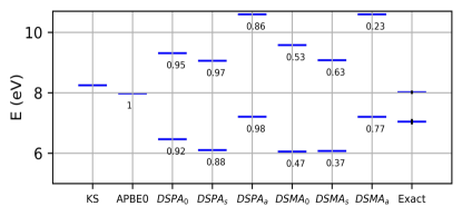
We next turn our attention to the Beryllium atom. Here the lowest two singlet states, have a mixed single and double excitation character. Ref. Loos et al. (2019) reports a roughly single-excitation character to the predominantly doubly-excited state (. As a result, adiabatic TDDFT fails to describe the states accurately. Figure 2 shows a plot of the two excitation frequencies of the multiplet. Adiabatic TDDFT with the PBE functional gives only one state in this frequency region which is closer in energy to the upper exact state, which would take up all the oscillator strength () within the SMA. The three flavors of DSMA give two states, but overestimate their energy splitting. Still, DSMA0 and especially DSMAS yield oscillator strengths which are close to that of the reference Ref. Loos et al. (2019) for the lower excitation, within the assumption that Be is weakly enough correlated that meaningfully approximates the single-excitation component of the state . On the other hand, the three flavors of DSPA also give two excitation frequencies but yield wrong oscillator strengths and violate the oscillator sum rule.
Finally we turn to the LiH molecule at stretched bond lengths, which we will use to illustrate the use of our DSMA to calculate coupling matrix elements between excited states. Adiabatic approximations to calculate these within quadratic response are plagued with unphysical divergences that appear when the difference between two excitation energies , and coincides with another excitation frequency Parker, Roy, and Furche (2016); Li and Liu (2014); Zhang and Herbert (2015); Ou et al. (2015) (see Supplementary Information for a figure of this). In Ref. Dar, Roy, and Maitra (2023) a frequency-dependent approximation for the second-order response kernel, , was derived in a truncated Hilbert space containing these states, that eliminated these divergences. This kernel was used to derive the transition density for a case where :
| (15) |
Here and are the frequencies of the dominant KS states contributing to the interacting levels and respectively, . In the case considered, state has predominantly single-excitation character, and a frequency-independent kernel suffices for this kernel. The third term involves , an adiabatic approximation to the second-order response kernel. The first term is the contribution from a double excitation, which should be weighted by the doubles contribution to state , which, in the limit of weak enough interaction is , however until the present work, how to calculate this was unknown. We note that Eq. (15) differs a little from that given in Ref. Dar, Roy, and Maitra (2023): there we had instead proposed to approximately weigh the doubles contribution with , where is a spatially-independent approximation to with and likewise is the product of the KS transition densities where we use the subscript to denote the KS state that the TDDFT state is dominated by, but the weights in Eq. (15) are better justified in the weak-interaction limit. In the specific application to the LiH transition dipole in Ref. Dar, Roy, and Maitra (2023), reproduced in the Supplementary Material here, only the second term was computed (with ), since the underlying linear response TDDFT calculation was done in the adiabatic approximation over all frequencies, so would not detect any double-excitation contribution. In reality, a KS double-excitation lies near (see Supplementary Material and also Fig. 3 shortly). The approximation of Ref. Dar, Roy, and Maitra (2023) has an overall trend that follows the exact results, but becomes an overestimate to the left of the resonance region while underestimating it to the right.
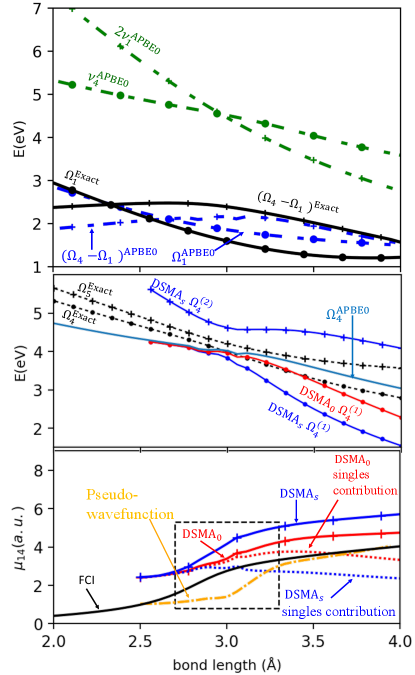
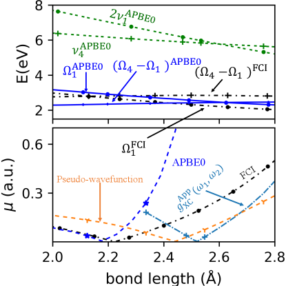
We now use DSMA to compute the proper weight associated with the first and second terms in Eq. (15) for the transition dipole moment between the 1st and 4th singlet excited states in LiH, , where is along the internuclear axis. In Fig. 3 all calculations are done in the aug-cc-pVDZ basis set using PySCF Sun et al. (2018), while the pseudo-wavefunction calculation is performed with the Turbomole package tur 111 The pseudo-wavefunction result was obtained using PBE0/aug-cc-pVDZ within the Turbomole package. To get smooth results in this basis, the computational parameters used were: SCF convergence threshold ; TDDFT residual threshold . As demonstrated in the Supplementary Material, both the TDDFT and reference Full Configuration Interaction (FCI) results show significant basis-set dependence; the transition dipole moments more so than the excitation energies, but convergence appears to be reached with the aug-cc-pVDZ basis. The top panel shows the intersection of the energy of the KS double-excitation with the 4th KS excitation frequency, justifying the need for the DSMA approach. The black lines demonstrate the “resonance condition" for FCI, , while near the intersection of the corresponding curves for APBE0 (blue lines), diverges (see Refs. Parker, Roy, and Furche (2016); Dar, Roy, and Maitra (2023) and Supplementary Material). The middle panel shows the 4th and 5th singlet excitation energies of the exact, and the one APBE0 excitation in this frequency-range, consistent with its blindness to the KS double-excitation in the top panel. Applying our DSMA to this 4th state, we retrieve two states, and , but with some error compared to the exact; both DSMAS and DSMAa overshoot the splitting between the two states, with the upper level of the latter being off the scale of the graph. The lowest panel compares computed from Eq. (15) ( using obtained from DSMA0 and DSMAS, against the reference FCI and the pseudo-wavefunction approximation Li and Liu (2014); Zhang and Herbert (2015); Ou, Alguire, and Subotnik (2015); Ou et al. (2015); Parker, Roy, and Furche (2016). The latter is often used to tame the divergence of the raw adiabatic transition dipole, but is somewhat ad hoc in that its underlying kernel structure is not yet known. In the indicated region of strong mixing between the single and double excitation , although they overestimate the dipole, DSMAS and especially DSMA0 both have a better trend as a function of and are closer to the FCI reference than the pseudo-wavefunction approach. The dotted curves indicate the importance of the double-excitation contribution.
By providing oscillator strengths and excitation energies of states of double-excitation character, the new kernel presented here improves the reliability of TDDFT for linear response spectra, as well as for quadratic response properties where it provides an otherwise missing contribution to the excited-to-excited state transition densities. Future work involves extensive tests on a range of systems including to cases when more than one single-excitation couples strongly with a double-excitation. Also, ramifications of Eq. (3) outside the problem of double excitations will be explored. For example, calculating oscillator strengths using an orbital-dependent functional (exact exchange, hybrids, meta-GGAs) within pure DFT imply a frequency-dependence and an analogous formula for the generalized KS framework may be needed.
Acknowledgements.
We warmly dedicate this article to John Perdew on his 80th birthday, as we continue to be guided by his development of approximations that yield "almost the right answer for almost the right reason for almost the right price" Kaplan, Levy, and Perdew (2023), the success of which in the field of materials science and quantum chemistry speaks for itself. We hope that this contribution is a step in this direction for the problem of oscillator strengths and excited state couplings with states of double-excitation character, and that John will enjoy reading it! We are very grateful to Shane Parker for providing us with the pseudowavefunction results, and to him and Filip Furche for useful discussions. Financial support from the National Science Foundation Award CHE-2154829 is gratefully acknowledged.I Three Flavors of Dressed Single Pole Approximation (DSPA)
The following are the three flavors of DSPA which were obtained by using the same substitutions as the ones used to get the three DSMA flavors in the main text:
| (1) |
| (2) |
| (3) |
where symbols have the same meaning as in the paper. Comparing Fig. 1 from the main text to Fig. S1 and Fig. S2 we observe that in terms of excited state frequencies, the corresponding DSPA and DSMA flavors are comparable, but DSMA is clearly superior to DSPA for the determination of oscillator strengths.
II LiH: Basis Set Dependence of FCI Results and Transition Dipole Moment from Quadratic Response TDDFT
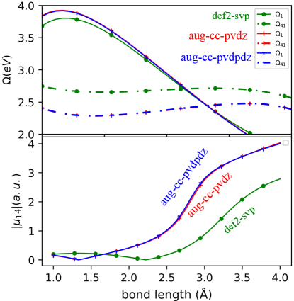
The full configuration interaction (FCI) results for the frequencies and transition dipole moment between the 1st and the 4th singlet excited state of LiH molecule in the main text appear quite different from those shown in Refs. Dar, Roy, and Maitra (2023); Parker, Roy, and Furche (2016), due to using a different basis set. The TDDFT results for the dipole moment, using adiabatic TDDFT, pseudowavefunction, or the frequency-dependent gXC kernel from Ref. Dar, Roy, and Maitra (2023) (Eq. (15) of main text) are all also quite sensitive to basis set, more so than the TDDFT energies. This should be borne in mind when comparing against a reference: given the different basis set sensitivities of different methods, thought needs to be given to which basis a FCI reference calculation should be compared to when gauging the accuracy of a TDDFT approximation performed in a given basis. To illustrate this, we compare the excited state frequencies and transition dipole moments given by the FCI within different basis sets in Fig. S3. Going from the def2-svp basis to the augmented Dunning basis sets aug-cc-pVDZ and aug-cc-pVDPDZ, the transition dipole moment shows more sensitivity than the excited state frequencies. Using progressively bigger basis sets in the augmented Dunning basis set series results in convergence for which we use as reference in the main paper.
Next, we reproduce the results of Ref. Dar, Roy, and Maitra (2023) which used the def2-SVP basis, to compare with the figure in the main text of the present paper that uses the aug-cc-pVDZ basis. Figure S4 shows the transition dipole moment between the 1st and 4th excited states of LiH molecule in the A1 irreducible representation of point group symmetry. The dipole is computed along the internuclear axis , as a function of bond-length using the adiabatic approximation, APBE0 within quadratic response TDDFT, the pseudo-wavefunction approach and using Eq. (15) of the main text by taking , as was done in Ref. Dar, Roy, and Maitra (2023). All calculations are done with def2-SVP basis set, using PySCF Sun et al. (2018) with the exception of pseudo-wavefunction which is done using the Turbomole package tur . As can be seen, in the region around 2.6 the 4th excited state frequency is close to twice the 1st excited state frequency (while in the larger aug-cc-pVDZ basis shown in the main text, the intersection appears closer to 2.6). Compared to the FCI shown in the lower panel, ABPE0 suffers from the expected divergence while the approximation, which lacks the proper oscillator strength fractions, effectively mitigates the divergence observed in the transition dipole moment obtained from the adiabatic approximation in the region where the resonance condition is satisfied. We see that the approximation aligns with the overall pattern observed in the exact results, however, it tends to overestimate the values to the far left of the resonance region while underestimating it to the right.
References
- Maitra (2022) N. T. Maitra, “Double and charge-transfer excitations in time-dependent density functional theory,” Annual Review of Physical Chemistry 73, 117–140 (2022), pMID: 34910562, https://doi.org/10.1146/annurev-physchem-082720-124933 .
- Loos et al. (2019) P.-F. Loos, M. Boggio-Pasqua, A. Scemama, M. Caffarel, and D. Jacquemin, “Reference energies for double excitations,” Journal of Chemical Theory and Computation 15, 1939–1956 (2019), https://doi.org/10.1021/acs.jctc.8b01205 .
- Jamorski, Casida, and Salahub (1996) C. Jamorski, M. E. Casida, and D. R. Salahub, “Dynamic polarizabilities and excitation spectra from a molecular implementation of time-dependent density-functional response theory: N2 as a case study,” J. Chem. Phys. 104, 5134–5147 (1996).
- Tozer and Handy (2000) D. J. Tozer and N. C. Handy, “On the determination of excitation energies using density functional theory,” Phys. Chem. Chem. Phys. 2, 2117–2121 (2000).
- Maitra et al. (2004) N. T. Maitra, F. Zhang, R. J. Cave, and K. Burke, “Double excitations within time-dependent density functional theory linear response,” J. Chem. Phys. 120 (2004).
- Hirata, Nooijen, and Bartlett (2000) S. Hirata, M. Nooijen, and R. J. Bartlett, “High-order determinantal equation-of-motion coupled-cluster calculations for electronic excited states,” Chemical Physics Letters 326, 255–262 (2000).
- Romaniello et al. (2009) P. Romaniello, D. Sangalli, J. A. Berger, F. Sottile, L. G. Molinari, L. Reining, and G. Onida, “Double excitations in finite systems,” J. Chem. Phys. 130, 044108 (2009).
- Sangalli et al. (2011) D. Sangalli, P. Romaniello, G. Onida, and A. Marini, “Double excitations in correlated systems: A many–body approach,” The Journal of Chemical Physics 134, 034115 (2011), https://doi.org/10.1063/1.3518705 .
- Bintrim and Berkelbach (2022) S. J. Bintrim and T. C. Berkelbach, “Full-frequency dynamical Bethe–Salpeter equation without frequency and a study of double excitations,” The Journal of Chemical Physics 156, 044114 (2022), https://pubs.aip.org/aip/jcp/article-pdf/doi/10.1063/5.0074434/16534759/044114_1_online.pdf .
- Damour et al. (2023) Y. Damour, R. Quintero-Monsebaiz, M. Caffarel, D. Jacquemin, F. Kossoski, A. Scemama, and P.-F. Loos, “Ground- and excited-state dipole moments and oscillator strengths of full configuration interaction quality,” Journal of Chemical Theory and Computation 19, 221–234 (2023), pMID: 36548519, https://doi.org/10.1021/acs.jctc.2c01111 .
- Sarkar et al. (2021) R. Sarkar, M. Boggio-Pasqua, P.-F. Loos, and D. Jacquemin, “Benchmarking td-dft and wave function methods for oscillator strengths and excited-state dipole moments,” Journal of Chemical Theory and Computation 17, 1117–1132 (2021), pMID: 33492950, https://doi.org/10.1021/acs.jctc.0c01228 .
- Cave et al. (2004) R. J. Cave, F. Zhang, N. T. Maitra, and K. Burke, “A dressed TDDFT treatment of the 21ag states of butadiene and hexatriene,” Chem. Phys. Lett. 389, 39 – 42 (2004).
- Elliott et al. (2011) P. Elliott, S. Goldson, C. Canahui, and N. T. Maitra, “Perspectives on double-excitations in TDDFT,” Chem. Phys. 391, 110 – 119 (2011).
- Huix-Rotllant et al. (2011) M. Huix-Rotllant, A. Ipatov, A. Rubio, and M. E. Casida, “Assessment of dressed time-dependent density-functional theory for the low-lying valence states of 28 organic chromophores,” Chem. Phys. 391, 120 – 129 (2011).
- Mazur and Włodarczyk (2009) G. Mazur and R. Włodarczyk, “Application of the dressed time-dependent density functional theory for the excited states of linear polyenes,” J. Comput. Chem. 30, 811–817 (2009).
- Mazur et al. (2011) G. Mazur, M. Makowski, R. Włodarczyk, and Y. Aoki, “Dressed TDDFT study of low-lying electronic excited states in selected linear polyenes and diphenylopolyenes,” Int. J. Quant. Chem. 111, 819–825 (2011).
- Dar, Roy, and Maitra (2023) D. Dar, S. Roy, and N. T. Maitra, “Curing the divergence in time-dependent density functional quadratic response theory,” The Journal of Physical Chemistry Letters 14, 3186–3192 (2023).
- Li and Liu (2014) Z. Li and W. Liu, “First-order nonadiabatic coupling matrix elements between excited states: A lagrangian formulation at the cis, rpa, td-hf, and td-dft levels,” The Journal of Chemical Physics 141, 014110 (2014).
- Zhang and Herbert (2015) X. Zhang and J. M. Herbert, “Analytic derivative couplings in time-dependent density functional theory: Quadratic response theory versus pseudo-wavefunction approach,” J. Chem. Phys. 142, 064109 (2015).
- Ou, Alguire, and Subotnik (2015) Q. Ou, E. C. Alguire, and J. E. Subotnik, “Derivative couplings between time-dependent density functional theory excited states in the random-phase approximation based on pseudo-wavefunctions: Behavior around conical intersections,” The Journal of Physical Chemistry B 119, 7150–7161 (2015).
- Ou et al. (2015) Q. Ou, G. D. Bellchambers, F. Furche, and J. E. Subotnik, “First-order derivative couplings between excited states from adiabatic TDDFT response theory,” J. Chem. Phys. 142, 064114 (2015).
- Parker, Roy, and Furche (2016) S. M. Parker, S. Roy, and F. Furche, “Unphysical divergences in response theory,” The Journal of Chemical Physics 145, 134105 (2016), http://dx.doi.org/10.1063/1.4963749 .
- Casida (1995) M. Casida, “Time-dependent density functional response theory for molecules,” in Recent Advances in Density Functional Methods, Part I, edited by D. Chong (World Scientific, Singapore, 1995).
- Petersilka, Gossmann, and Gross (1996) M. Petersilka, U. J. Gossmann, and E. K. U. Gross, “Excitation energies from time-dependent density-functional theory,” Phys. Rev. Lett. 76, 1212–1215 (1996).
- Grabo, Petersilka, and Gross (2000) T. Grabo, M. Petersilka, and E. Gross, “Molecular excitation energies from time-dependent density functional theory,” Journal of Molecular Structure: THEOCHEM 501, 353–367 (2000).
- Gross and Maitra (2012) E. K. Gross and N. T. Maitra, “Introduction to TDDFT,” in Fundamentals of time-dependent density functional theory, Vol. 837, edited by M. A. Marques, N. T. Maitra, F. M. Nogueira, E. K. Gross, and A. Rubio (Springer, 2012) pp. 53–97.
- Hirata and Head-Gordon (1999) S. Hirata and M. Head-Gordon, “Time-dependent density functional theory within the tamm–dancoff approximation,” Chemical Physics Letters 314, 291–299 (1999).
- Liang et al. (2022) J. Liang, X. Feng, D. Hait, and M. Head-Gordon, “Revisiting the performance of time-dependent density functional theory for electronic excitations: Assessment of 43 popular and recently developed functionals from rungs one to four,” Journal of chemical theory and computation 18, 3460–3473 (2022).
- Casida et al. (2000) M. E. Casida, F. Gutierrez, J. Guan, F.-X. Gadea, D. Salahub, and J.-P. Daudey, “Charge-transfer correction for improved time-dependent local density approximation excited-state potential energy curves: Analysis within the two-level model with illustration for H2 and LiH,” The Journal of Chemical Physics 113, 7062–7071 (2000), https://pubs.aip.org/aip/jcp/article-pdf/113/17/7062/10826979/7062_1_online.pdf .
- Carrascal et al. (2018) D. Carrascal, J. Ferrer, N. Maitra, and K. Burke, “Linear response time-dependent density functional theory of the hubbard dimer,” The European Physical Journal B 91, 142 (2018).
- Chrayteh et al. (2021) A. Chrayteh, A. Blondel, P.-F. Loos, and D. Jacquemin, “Mountaineering strategy to excited states: Highly accurate oscillator strengths and dipole moments of small molecules,” Journal of Chemical Theory and Computation 17, 416–438 (2021), pMID: 33256412, https://doi.org/10.1021/acs.jctc.0c01111 .
- Robinson (2018) D. Robinson, “Comparison of the transition dipole moments calculated by tddft with high level wave function theory,” Journal of Chemical Theory and Computation 14, 5303–5309 (2018), pMID: 30068079, https://doi.org/10.1021/acs.jctc.8b00335 .
- Caricato et al. (2011) M. Caricato, G. W. Trucks, M. J. Frisch, and K. B. Wiberg, “Oscillator strength: How does tddft compare to eom-ccsd?” Journal of Chemical Theory and Computation 7, 456–466 (2011), pMID: 26596165, https://doi.org/10.1021/ct100662n .
- Laurent and Jacquemin (2013) A. D. Laurent and D. Jacquemin, “Td-dft benchmarks: A review,” International Journal of Quantum Chemistry 113, 2019–2039 (2013), https://onlinelibrary.wiley.com/doi/pdf/10.1002/qua.24438 .
- Sun et al. (2018) Q. Sun, T. C. Berkelbach, N. S. Blunt, G. H. Booth, S. Guo, Z. Li, J. Liu, J. D. McClain, E. R. Sayfutyarova, S. Sharma, et al., “Pyscf: the python-based simulations of chemistry framework,” Wiley Interdisciplinary Reviews: Computational Molecular Science 8, e1340 (2018).
-
(36)
“TURBOMOLE V7.2 2017, a development of University of Karlsruhe and Forschungszentrum Karlsruhe GmbH, 1989-2007, TURBOMOLE GmbH, since 2007; available from
http://www.turbomole.com.” . - Note (1) The pseudo-wavefunction result was obtained using PBE0/aug-cc-pVDZ within the Turbomole package. To get smooth results in this basis, the computational parameters used were: SCF convergence threshold ; TDDFT residual threshold .
- Kaplan, Levy, and Perdew (2023) A. D. Kaplan, M. Levy, and J. P. Perdew, “The predictive power of exact constraints and appropriate norms in density functional theory,” Annual Review of Physical Chemistry 74, 193–218 (2023), pMID: 36696591, https://doi.org/10.1146/annurev-physchem-062422-013259 .