Oscillations in weighted arithmetic sums
Abstract.
We examine oscillations in a number of sums of arithmetic functions involving , the total number of prime factors of , and , the number of distinct prime factors of . In particular, we examine oscillations in and in for , and in . We show for example that each of the inequalities , , , and is true infinitely often, disproving some hypotheses of Sun.
Key words and phrases:
Prime-counting functions, Liouville function, oscillations, Riemann hypothesis2010 Mathematics Subject Classification:
Primary: 11M26, 11N64; Secondary: 11Y35, 11Y701. Introduction
Let denote the number of distinct prime factors of , and let denote its total number of prime factors, counting multiplicity. Questions involving the parity of these functions have a long history. For , define
| (1.1) |
and
| (1.2) |
Pólya studied in his 1919 article [23]. He noted that was not positive after up to approximately , and remarked that the Riemann hypothesis, as well as the simplicity of the zeros of the zeta function, would follow if this held true for all sufficiently large . More generally, it is well known that both of these statements would hold if the normalized function were bounded by some constant, either above or below. In his influential 1942 paper [14], Ingham showed that considerably more would follow in this case: there would exist infinitely many linear dependencies over the rationals among the ordinates of the zeros of the zeta function on the critical line in the upper half plane. Stated another way, if the (positive) ordinates of the nontrivial zeros of are linearly independent, then arbitrarily large oscillations must exist in . In fact, Ingham showed that this holds both for Pólya’s function and for its close cousin, the Mertens function,
| (1.3) |
Since it seems there is no a priori reason to suspect such linear dependencies, and none has ever been detected among the zeros of the zeta function, it is often conjectured that these functions exhibit unbounded oscillations. Large oscillations have been shown to exist in the Mertens function [4, 13] and in the error term for the distribution of -free numbers [19].
Turán studied in 1948 [25], where he reported that this function is never negative over , and connected its behavior to the zeros of the Riemann zeta function. Here, the Riemann hypothesis, as well as the simplicity of the zeros and the existence of linear dependencies among their ordinates, would similarly follow if were bounded either above or below. Haselgrove [11] established that infinitely many sign changes in both and exist. Specific locations of sign changes in these functions were first determined respectively in [16] and in [6].
The broader family was investigated in [20], where the authors established how these functions are connected to the Riemann hypothesis, as well as the statement on the simplicity of the zeros of and the question of linear independence. In [21] it was shown that substantial oscillations must exist in the normalized functions . For example, it was shown that each of the inequalities and holds for infinitely many integers (see [21, Thms. 1.1 and 6.2]). The reader is referred to [6, 12, 20, 21] for additional information and background on this family of functions.
In [22], the authors established similar connections and statements for the function . Here, among other things, it was established that each of the inequalities and holds for infinitely many positive integers .
In [24, Conj. 1.1], Sun hypothesized that both and are for any . Both of these statements seem likely to be true, since either of these is equivalent to the Riemann hypothesis (see also [5, 20]). Sun also remarked there that may be , but by the same argument employed in [21, §5] for , bounding would again imply the existence of infinitely many linear dependence relations among the ordinates of the zeros of the zeta function in the upper half plane, so a bound of this strength seems doubtful.
In this paper, we prove that large oscillations must exist in for every . This presents an -complement to the work of [20] and [21], and generalizes the oscillation result concerning the case from [22] in a natural way. For and , let denote the Dirichlet series
| (1.4) |
The series was investigated by van de Lune and Dressler in 1975 [18], who proved that its value is . Following [22, §5], we may write the Euler product above as
| (1.5) |
where
is an explicitly given function that converges in the half plane , and
so that can be continued analytically to the left of the line. (We remark as in [22] that there is no trouble in extending the form in (1.5) so that the corresponding function converges on for larger values of .) For convenience we write in place of for throughout. For , we define by
| (1.6) |
We establish the following theorem.
Theorem 1.1.
For each , each of the following inequalities holds for infinitely many positive integers :
Sun made some additional conjectures regarding sums involving in [24], which we also address here. Let
| (1.7) |
In [24, Hypoth. 1.1], Sun made the following four hypotheses:
| (1.8) | |||
| (1.9) | |||
| (1.10) | |||
| (1.11) |
Certainly (1.10) and (1.11) are stronger than (1.8) and (1.9) respectively for sufficiently large , and clearly (1.10) and (1.11) appear related. Sun reported that (1.10) was checked for and (1.11) for .
We disprove all four of these statements in this article. In two of the conjectured inequalities above—the lower bounds in (1.10) and (1.11)—we also determine the minimal counterexample, after calculating these functions for . We summarize some of the results of our computations in the following theorem.
Theorem 1.2.
The following statements hold for the function from (1.7).
-
(a)
The smallest integer for which is . Here, , so .
-
(b)
The minimal value of for integers with is , occurring at , and .
-
(c)
The smallest integer for which is , at which .
-
(d)
The minimal value of for integers occurs at , and .
In addition, we determine lower bounds on the oscillations exhibited by and . These results show that each of the conjectured bounds in (1.8), (1.9), (1.10), and (1.11) is violated infinitely often. Our method in fact allows us to determine information on for any . For this, we define
| (1.12) |
We determine bounds on oscillations for for all in the following theorem.
Theorem 1.3.
For each , each of the following inequalities is satisfied for infinitely many positive integers :
| (1.13) |
In particular, each of the following holds for infinitely many positive integers :
| (1.14) |
In addition, each of the following inequalities is satisfied for infinitely many positive integers :
| (1.15) |
In this article we investigate another conjecture made by Sun as well in [24]. Let
| (1.16) |
The similar function was considered by Grosswald [8] and by Bateman [2]: in particular, Grosswald proved that . In [24, Conj. 1.1] Sun conjectured that a smaller and explicit bound holds for :
| (1.17) |
We investigate this function here, and verify that (1.17) holds for .
This article is organized in the following way. Section 2 describes the notion of weak independence of a set of real numbers, and its use in establishing lower bounds on the oscillation of sums of certain arithmetic functions. Section 3 presents the analysis of the functions , and establishes Theorem 1.3. Following this, Section 4 considers the family , and proves Theorem 1.1. Details on the computations that establish Theorem 1.2 and related facts, along with information on calculations for , are described in Section 5. Finally, in Section 6 we touch on some other conjectures of Sun from [24].
2. Weak independence and oscillations
The work of Grosswald [9, 10], Bateman et al. [3], Diamond [7], Anderson and Stark [1], and others establishes connections between bounding oscillations in sums of certain arithmetic functions and the existence of integral linear relations among the ordinates of nontrivial zeros of , where the linear relations have bounded coefficients. For example, in 1971 Bateman et al. [3] showed that if the Mertens function (1.3) satisfied for all then there would exist infinitely many linear relations among the nontrivial zeros of in the upper half plane with maximum coefficient . They showed as well that the ordinates of the first zeros of on the critical line are -independent, that is, there exist no nontrivial linear relations among these values using coefficients . In a more recent study of oscillations in the Mertens function [4], it was shown that the first zeros of are -independent.
Here, in order to exhibit large oscillations in sums we require a particular form of weak linear independence for certain zeros of . We assume the Riemann hypothesis and the simplicity of its zeros here and throughout this paper, as unbounded oscillations would follow anyway if either of these conditions did not hold. Let denote a set of positive real numbers, and for let denote a subset of . For each , let denote a positive integer. We say is -independent in if two conditions hold. First, whenever
then necessarily all . Second, for any , if
then , , and all other . That is, the only linear relations with small coefficients here are the trivial ones. In addition, if is a positive integer with the property that each with as above, then we say that is -independent in .
Anderson and Stark [1] established a means for bounding oscillations by using weak independence. We summarize a particular result of theirs: suppose is a piecewise continuous, real function, bounded on finite intervals, with Laplace transform ,
Suppose also that is absolutely convergent in for some , and can be analytically continued back to , except for simple poles occurring at for , for a particular set of positive real numbers, and possibly a simple pole at as well. If is -independent in , then
| (2.1) |
where denotes an admissible weight function, which must be even, nonnegative, supported on , have the value at , and be the Fourier transform of a nonnegative function. While the Fejér kernel ( for and otherwise) is admissible, we employ the kernel of Jurkat and Peyerimhoff [15] here, defined by
| (2.2) |
This kernel provides more weight to values of near the origin compared to the Fejér kernel (and correspondingly less weight to values farther away), and this is often advantageous.
The result (2.1) then provides a weak version of Ingham’s theorem for the case of weak independence. Ingham established a result similar to (2.1), where linear independence over the rationals for was required, the fractions were naturally omitted, and was replaced by .
The LLL lattice reduction algorithm [17], combined with some additional linear algebra, may be employed to establish weak independence of a finite set of positive real numbers, relative to a parent set and a real parameter . In this article, we are able to employ some weak independence results established in prior work, so we omit a detailed description of the algorithm, and refer the reader to the following sources. The article [20] provides a detailed explanation of Ingham’s method, extended to the family of functions from (1.1), including connections with the Riemann hypothesis, the simplicity of the zeros of the zeta function, and the linear independence question. The publications [4, 19, 21, 22] describe the method of weak independence, and computational strategies for establishing this property. The first of these treats the Mertens function , the third deals with the family , and the last one considers from (1.2). In particular, the paper [21] contains substantial exposition on this method, including for example a proof of (2.1).
3. Oscillations in
Since from (1.7) is rather similar to Pólya’s function , one might begin by employing some analysis similar to that of [20] and [21]. Indeed, when there is a simple relationship connecting these two functions:
Thus, we might expect to exhibit a bias with sign opposite to that of , and we might hope that methods that established large oscillations in might also produce similarly good results for . Indeed, this turns out to be the case, as we show below.
Let denote the Dirichlet series
If , then it is straightforward to establish that
This was also given by Sun [24]. Standard results (see, e.g., [20]) show that if either the Riemann hypothesis is false or a zero of is not simple, then
Hence we may assume the Riemann hypothesis and the simplicity of the zeros in order to exhibit large oscillations. We follow the same procedure as in [20]. With as in (1.12), we define
The Laplace transform of is
and as in [20] we compute
| (3.1) |
where
| (3.2) |
The adjustments made to when creating in (1.12) are engineered so that the function in (3.1) is analytic in the open half-plane with only simple poles on the imaginary axis. In particular, the adjustment at removes the pole of order at in (3.2), and the adjustment for removes the simple pole on the real axis at . This prepares us to employ the result of Anderson and Stark and the machinery of weak independence.
For , we compute
| (3.3) |
where denotes Euler’s constant. For , where is the th zero of the zeta function on the critical line in the upper half plane, we have
| (3.4) |
If and is -independent in , then using the result of Anderson and Stark (2.1) (where ) we conclude that
| (3.5) |
In particular, when , this produces (writing )
| (3.6) |
for an infinite sequence of , and likewise
| (3.7) |
for another infinite sequence of . Note that , so that, in a loose sense, one expects to be biased towards positive values. Similarly, exhibits the same oscillation bounds about , since . We note that the conjectures (1.10) and (1.11) are the same as stating that the magnitude of the oscillations here never exceeds approximately , since and .
We may now complete the proof of Theorem 1.3 by employing a result on weak independence.
Proof of Theorem 1.3.
In [21], we determined a particular set having with the property that is -independent in . Employing this set in (3.6) and (3.7), and using the kernel of Jurkat and Peyerimhoff (2.2), produces oscillations with magnitude in each direction. Since for , the first statement follows. The subsequent statements for and in (1.14) recapitulate the inequalities in (1.13) for these cases. However, the statements for and employ the oscillation bounds from (3.5) computed as for these cases. Likewise, the final statement (1.15), regarding the case , employs the computed oscillation bound of for this case (which is in fact maximal over ), together with the appropriate entries from (1.12) and (3.3). ∎
We remark that it is possible to improve the bounds in Theorem 1.3 with a new computation, using zeros selected to maximize contributions according to the residues (3.4) in this problem, rather than employing the set of residues that were selected for the functions . However, we would not witness a substantial gain with a calculation of approximately the same size: we estimate gaining in the oscillation bound in each direction from a computation with approximately zeros. This computation would require several months of core time, so with a high cost relative to a small benefit we opted against a new calculation here.
4. Oscillations in
In order to prove Theorem 1.1, we generalize our analysis in [22], in a manner analogous to the prior section and our study of the behavior from [20] and [21]. In [22], for the case we computed the Laplace transform of : under the Riemann hypothesis, this function is analytic in the half plane . For the general case, we proceed in a similar manner, except that when one must incorporate an adjustment to prevent the appearance of a pole on the positive real axis in the corresponding Laplace transform. In essence one must account for the value of for , with defined in this interval by (1.5). We made precisely the analogous adjustment in the analysis of in [20] and [21]. Using the function from (1.6), for we set to be a suitable scaling of :
Next, we set
| (4.1) |
and
Using an argument very similar to that employed in [20] for , we find that for all , the function is the Laplace transform of :
| (4.2) |
and, under the Riemann hypothesis, the integral in (4.2) converges for all . One slight difference arises here: when there is a pole of in (4.1) when . However, this is canceled by the zero of , which itself comes from the pole of in (1.5). As such, unlike the case of or , there is no dramatic bias in .
It is now straightforward to calculate the residue of at each pole along . We have
| (4.3) |
From (4.3) and the fact that , we expect no bias in the sum for and for . Over , we expect a bias in this function whenever . Figure 1 exhibits over . It is interesting that the sign of the bias changes over this range. For , our plot indicates that we expect to exhibit a negative bias, with maximal negative bias occurring near , where . That is, the values of will oscillate relative to the base curve . For , we expect the sum to display a positive bias, with maximal bias occurring near , where . Figure 7 displays for two values of near these points of maximal bias. In these plots, the bias specified by was not removed as in (1.6), so in each of these graphs the oscillations center on an exponential function. In part (b) of this figure, where , the bias is quite evident, since the centering curve is . However, in part (a) it is not so obvious, since the guiding exponential remains rather small over the plotted interval.

We may now establish Theorem 1.1 by computing the relevant residues and employing a particular set of zeros of the zeta function known to possess a weak independence property.
Proof of Theorem 1.1.
In [22], we computed the residue of at each of its simple poles on the imaginary axis, so at each point where denotes the th zero of the Riemann zeta function on the critical line in the upper half plane. This derivation generalizes in a natural way and yields
The same article employed a particular set of ordinates of zeros of the zeta function on the critical line, with , to establish large oscillations for . By proving that is -independent in with , we obtained Theorem 1.1 from (2.1) in the case , since
| (4.4) |
Theorem 1.1 follows almost immediately. Since for , certainly
over this range, and thus the bound (4.4) holds as well when is replaced by , for any . ∎
We remark that since , we see that , so the bound for is in fact exactly the same as that for for . In particular, the bound for , which was of particular interest in [24], matches the one for . We add also that our method establishes bounds on oscillations for that are only slightly stronger than (4.4). In the most beneficial case (when ), we obtain
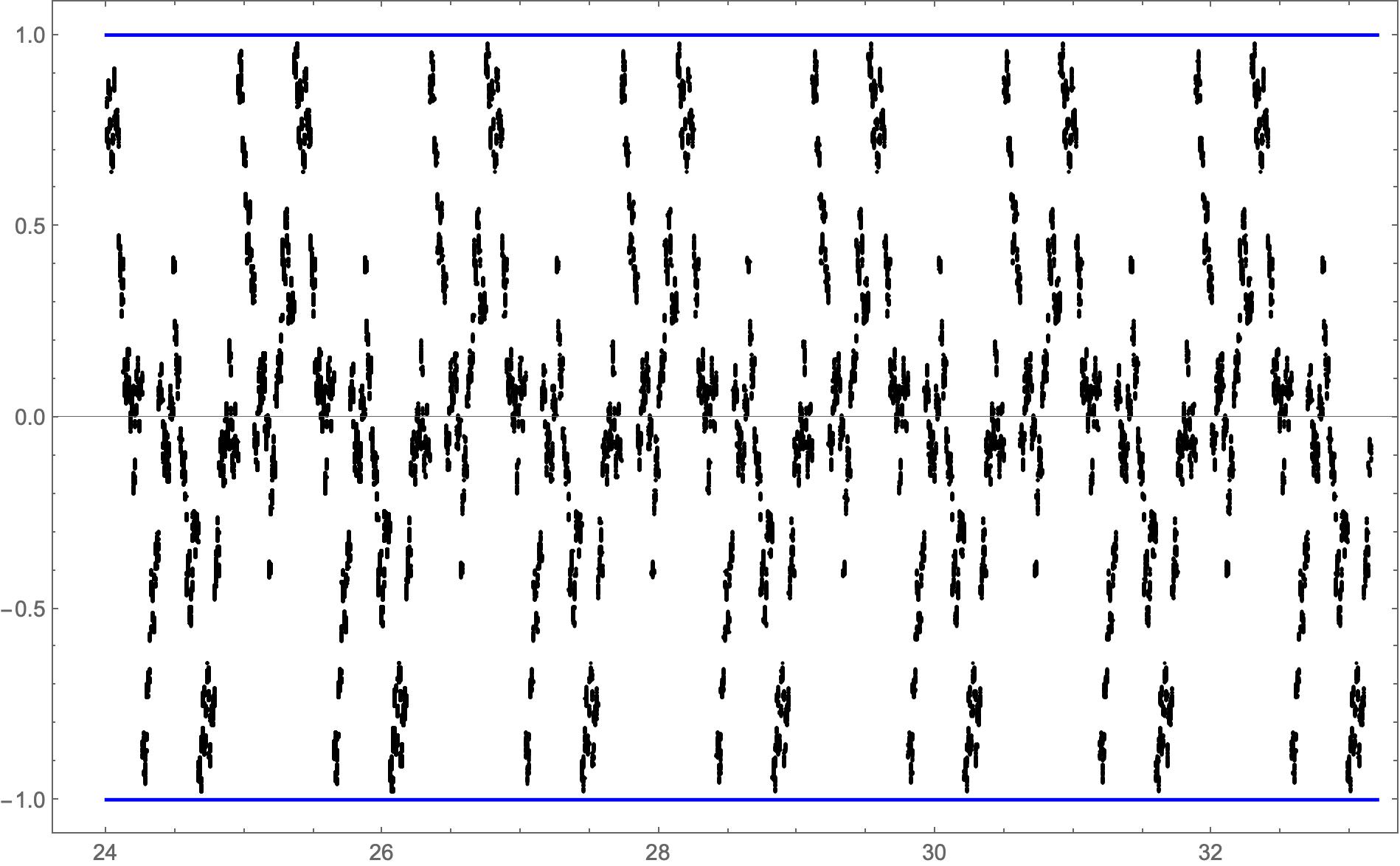
Figure 6 displays plots of for a number of values of . These plots were obtained from sampling the values of these functions for . The graphs also display the axes where the oscillations are centered. In part (d) of this figure, where , the axis is the horizontal line at ; for the others it is the horizontal axis.
5. Computations
We completed a number of computations to sample the values of and for several choices of the parameter , as well as from (1.16). Our method is similar to the one developed in [6] for the investigation of and ; a similar method was employed in [21] for and in [22] for . We summarize the method used here for obtaining values of the functions , in order to provide information for Theorem 1.2.
By using Perron’s formula and the procedure of [20], we find that
| (5.1) |
where the error term satisfies as . We use this to estimate the behavior of , by setting in (5.1) and calculating the expression on the right with set to certain values, and then plotting the results. When , so with zeros of the zeta function in the upper half plane, we detected a potential crossing point for the lower bound in (1.10)—see Figure 2(a). This suggests that may dip below near , and similarly may cross the lower threshold of from (1.11) near the same location. These values seemed within range of a distributed computation, so we aimed to calculate and for .
 |
 |
| (a) () | (b) () |


To calculate values for , we first created a large table to store the parity of the values of for all positive integers with and . This required about gigabytes of storage. We employed a boot-strapping strategy to create this table: once the values up to a bound have been computed, we can then sieve the interval using the primes to determine the parity of the total number of divisors for each qualifying integer in this interval. Here we use the existing table for whenever a remaining cofactor lands in this interval, once powers of , , and are properly accounted for. After the full table to has been constructed, we launch a distributed calculation, with each processor employing a copy of the table to assist with sieving its own portion of the targeted range. Each process handled an interval of size , usually breaking this up into subintervals of size million in order to make efficient use of memory, as it was advantageous in scheduling to control the total memory size of each job. Two bits per integer were required during the sieving process, to record the parity of at location , or to indicate that the value at is not yet known, so a subinterval required megabytes of memory.
When a process sieves an interval , it first sieves using primes , working from the largest primes downward, since removing such a prime from any integer in this interval produces a cofactor in the stored table for , after removing any factors of , , and . After this we sieve with the primes , starting again with the largest primes and working downwards. The cofactor remaining after removing all factors of such a prime may still exceed , so we employ trial division beginning with until the remaining cofactor is less than , or has been determined to be prime. After this, the remaining unknown elements in the current interval must have the form with or prime, and some final scans take care of these. Cumulative totals are computed at the conclusion of each subinterval, and sampled values are occasionally produced as output. These sampled values record cumulative totals relative to the start of the large interval handled by the current process. At its conclusion, a process records cumulative totals over its entire run, and once all processes are completed these partial sums may be used to adjust the sampled values produced across the entire computation.
The same strategy was employed to compute values of for , , , and , although here we accumulated the positive and negative contributions separately to guard against loss of precision.
Our computations allowed us to establish Theorem 1.2. Record high and low values were recorded for each interval of size handled by a process, and this produced the record values in parts (b) and (d) of this theorem. For each of parts (a) and (c), we needed to run an additional job to determine the precise first crossing points, once the true value of each process’ starting point was known.
Figures 3 and 4 exhibit our results for sampling over for the functions and . These plots also show the center of the oscillations , and the conjectured bounds from (1.10) and (1.11). In each plot, the crossing in the conjectured lower bounds in these inequalities near is evident.

No violations of the upper bound in (1.10) or (1.11) were found in this computation; the closest point was
which achieves , and is visible as a near-miss in Figure 3. A similar near-miss occurs for as seen in Figure 4. However, further experimentation with (5.1) suggested a potential location for such crossings. Figure 2(b) illustrates a crossing for the estimate from this expression when , so using zeros of the zeta function, near , or approximately . This is well beyond our present computational range.
Our strategy was similar for computing , for a number of values of , with suitable adjustments to the code to track the parity of rather than . Figure 6 exhibits plots for for several values of .
 |
 |
 |
||||
| (a) | (b) | (c) | ||||
|
||||||


 |
 |
| (a) , | (b) , |
A similar strategy was employed to compute values of up to , although here the table size was , since we now required four bits to store the value of at each location in this interval, rather than simply its parity (note ). This table then required about gigabytes of memory. During the sieving stage, each process allocated one byte per integer in each sieving block, since , so a subinterval required megabytes of storage. We find that Sun’s conjecture (1.17) survives over this range: the maximum value of for integers occurs at , where the ratio is ; the minimum value occurs at , where it is . We report a few additional values in Table 1, including the best value achieved in each direction for . Figure 8 displays over .
We note that the function may be amenable to some further analysis. As in (1.4), the corresponding Dirichlet function in this case is
for , and using methods similar to that employed to create (1.5) for , one may show that
where
which converges for . The function has poles of order on the imaginary axis, as well as one of order at the origin. We can manipulate this to ensure that the result of Anderson and Stark (2.1) is applicable. However, some additional complications arise, which we hope to address in future work.
6. Other conjectures
Sun made two additional families of conjectures concerning the quantity . First, in [24, Conj. 1.2], Sun opined that for , , or , the proportion of integers having the property that exceeds , provided that , for a particular quantity . For example, it was conjectured that , , and all suffice. For , this proportion was posited to be bounded above by , for . No conjecture was made in the case , although it was remarked that perhaps this proportion is infinitely often less than , and infinitely often greater. We verified that Sun’s seventeen conjectures here hold for . We can also report that the last crossing in the case over this range occurs at : from here to the proportion of integers having exceeds .
Second, in [24, Conj. 1.3] Sun stated a conjecture regarding a variant of twisted by Dirichlet characters. For or mod , let denote the Kronecker symbol, and let
Sun posited for example that
with sufficing in each case. In fact, additional conjectures of this form for other values of were stated as well. These could all be investigated by using results on -independence of zeros of the Dirichlet -function where is the non-principal character modulo . We know of no calculation, similar to that for in [3, 4], that establishes good -independence for Dirichlet -functions, although Grosswald [10, Thm. 5 and §8, §9] presents some calculations to this end. Such a program of research appears both possible and interesting: we hope to return to this in future work.
Acknowledgments
We thank Peter Humphries for bringing these questions to our attention, and we thank the referee for a number of helpful comments. We also thank NCI Australia and UNSW Canberra for computational resources. This research was undertaken with the assistance of resources and services from the National Computational Infrastructure (NCI), which is supported by the Australian Government.
References
- [1] R. J. Anderson and H. M. Stark. Oscillation theorems. Lecture Notes in Math., 899:79–106, 1981. MR0654520 (83h:10082)
- [2] P. T. Bateman. Proof of a conjecture of Grosswald. Duke Math. J., 25:67–72, 1958. MR0091970 (19,1040a)
- [3] P. T. Bateman, J. W. Brown, R. S. Hall, K. E. Kloss, and R. M. Stemmler. Linear relations connecting the imaginary parts of the zeros of the zeta function. Computers in Number Theory (Proc. Sci. Res. Council Atlas Sympos. No. 2, Oxford, 1969), 1971, pp. 11–19. MR0330069 (48 #8408)
- [4] D. G. Best and T. S. Trudgian. Linear relations of zeroes of the zeta-function. Math. Comp., 84(294): 2047–2058, 2015. MR3335903
- [5] O. Bordellès. Review of [24], MathSciNet.
- [6] P. Borwein, R. Ferguson, and M. J. Mossinghoff. Sign changes in sums of the Liouville function. Math. Comp., 77(263):1681–1694, 2008. MR2398787 (2009b:11227)
- [7] H. G. Diamond. Two oscillation theorems. In The theory of arithmetic functions (Proc. Conf., Western Michigan Univ., Kalamazoo, Mich., 1971), 1972, Springer, Berlin, pp. 113–118. MR0332684 (48 #11010)
- [8] E. Grosswald. The average order of an arithmetic function. Duke Math. J., 23:41–44, 1956. MR0074459 (17,588f)
- [9] E. Grosswald. Oscillation theorems of arithmetical functions. Trans. Amer. Math. Soc., 126:1–28, 1967. MR0202685 (34 #2545)
- [10] E. Grosswald. Oscillation theorems. Lecture Notes in Math., 251:141–168, 1972. MR0332685 (48 #11011)
- [11] C. B. Haselgrove. A disproof of a conjecture of Pólya. Mathematika, 5:141–145, 1958. MR0104638 (21 #3391)
- [12] P. Humphries. The distribution of weighted sums of the Liouville function and Pólya’s conjecture. J. Number Theory, 133(2):545–582, 2013. MR2994374
- [13] G. Hurst. Computations of the Mertens function and improved bounds on the Mertens conjecture. Math. Comp., 87(310):1013–1028, 2018. MR3739227
- [14] A. E. Ingham. On two conjectures in the theory of numbers. Amer. J. Math., 64(1):313–319, 1942. MR0006202 (3,271c)
- [15] W. Jurkat and A. Peyerimhoff. A constructive approach to Kronecker approximations and its application to the Mertens conjecture. J. Reine Angew. Math., 286/287:322–340, 1976. MR0429789 (55 #2799)
- [16] R. S. Lehman. On Liouville’s function. Math. Comp., 14:311–320, 1960. MR0120198 (22 #10955)
- [17] A. K. Lenstra, H. W. Lenstra, Jr., and L. Lovász. Factoring polynomials with rational coefficients. Math. Ann., 261(4):515–534, 1982. MR0682664 (84a:12002)
- [18] J. van de Lune and R. E. Dressler. Some theorems concerning the number theoretic function . J. Reine Angew. Math, 277:117–119, 1975. MR0384726 (52 #5599)
- [19] M. J. Mossinghoff, T. Oliveira e Silva and T. S. Trudgian. The distribution of -free numbers. Math. Comp., to appear. Preprint available at arXiv:1912.04972, 2020.
- [20] M. J. Mossinghoff and T. S. Trudgian. Between the problems of Pólya and Turán. J. Aust. Math. Soc., 93(1-2):157–171, 2012. MR3062002
- [21] M. J. Mossinghoff and T. S. Trudgian. The Liouville function and the Riemann hypothesis. In Exploring the Riemann Zeta Function, H. L. Montgomery et al. (eds.), 2017, Springer, Cham, pp. 201–221. MR3700043
- [22] M. J. Mossinghoff and T. S. Trudgian. A tale of two omegas. In 75 Years of Mathematics of Computation, S. C. Brenner, I. Shparlinski, C.-W. Shu, and D. B. Szyld, eds., Contemp. Math. 754, Amer. Math. Soc., Providence, RI, 2020, pp. 343–364. MR4132130
- [23] G. Pólya. Verschiedene Bemerkungen zur Zahlentheorie. Jahresber. Deutsch. Math.-Verein., 28:31–40, 1919.
- [24] Z.-W. Sun. On a pair of zeta functions. Int. J. Number Theory, 12(8): 2323–2342, 2016. MR3562029
- [25] P. Turán. On some approximative Dirichlet-polynomials in the theory of the zeta-function of Riemann. Danske Vid. Selsk. Mat.-Fys. Medd., 24(17): 1–36, 1948. MR0027305 (10,286a)