Origin of band flatness and constraints of higher Chern numbers

Electronic band flatness is a new condensed matter paradigm. The flat bands had been studied in the context of Landau levels Landau (1930); *Landau1977; Haldane (2018); Kapit and Mueller (2010); however a conceptually new approach in material science is engineering flat bands from the first principles Miyahara et al. (2005); Maimaiti et al. (2017); Rhim and Yang (2019). To date, we have accumulated sufficient numerical evidence of flat bands formation ranging from artificial crystallographic lattices (Kagome, Lieb) to controllable flat band engineering in twisted van der Waals heterostructures Trambly de Laissardière et al. (2010); Naik and Jain (2018); Carr et al. (2020). The controllable and predictable engineering of band flatness is of strategical importance, especially for strongly correlated phases such as unconventional superconductivity Cao et al. (2018); Yankowitz et al. (2019); Park et al. (2021); Hao et al. (2021), Fractional Chern Insulators Neupert et al. (2011); Tang et al. (2011); Sun et al. (2011); Haldane (2011), and the SYK phase Kitaev (2015); Sachdev and Ye (1993); Chen et al. (2018), to name a few. Of particular importance are flat Chern bands, however the higher-order Chern numbers are a rare case in reality, with the majority of natural flat bands restricted to $|C|=1$.

Generic construction of flat bands.—Consider a generic tight binding Hamiltonian $\mathcal{H}=\sum_{ij}^{\Lambda}t_{ij}^{\alpha\beta}c^{{\dagger}}_{i\,\alpha}c^{{\dagger}}_{j\,\beta}$. Here $\Lambda$ is the hopping range. Setting here lattice constant $a$$\to$$\infty$ (or $t_{ij}$$=$$0$) immediately recovers the ”atomic insulator”, a system with a perfectly flat band at $E_{0}$$=$$0$. The atomic insulator is the simplest perfectly flat band opening the ”periodic table” of perfectly flat bands (Table I). We can systematically build other classes of flat bands from the tight binding. In the momentum representation the generic tight-binding Hamiltonian reads $\mathcal{H}=\sum_{\mathbf{k}}c^{{\dagger}}_{\mathbf{k}\alpha}\mathcal{H}_{\alpha\beta}(\mathbf{k})c_{\mathbf{k}\beta}$. The matrix Hamiltonian $\mathcal{H}_{\alpha\beta}(\mathbf{k})$ has electronic bands $\varepsilon_{1}(k),\varepsilon_{2}(k)...\varepsilon_{N}(k)$. Among them, we pick up the $n$${}^{\text{th}}$ band which is dispersive, gapped out from the others, and not crossing zero. We further introduce a new Hamiltonian hosting the perfectly flat band through procedure

Band flatness for topologically-trivial bands. Addressing localization properties is more natural in terms of Wannier functions. Topologically-trivial flat bands are maximally Wannierizable, thus without loss of generality we consider localization along one of the two spatial dimensions and investigate its asymptotics Kohn (1959); He and Vanderbilt (2001)

Band flatness for Chern bands. We start from the construction of higher-$C$ Chern bands on the basis of double periodic meromorphic functions. The essential toolbox is built upon implementation of theta functions, Weierstrass and Jacobi functions, and their combinations Akhiezer (sian). Independently of the choice of the elliptic function, we can use connection between the wave function singularities (poles) and the band Chern number $C$$=$$\int_{\text{BZ}}\frac{d^{2}\mathbf{k}}{2\pi}F_{xy}$, with $F_{xy}$$=$$\partial_{x}A_{y}$$-$$\partial_{y}A_{x}$, $\mathbf{A}_{\mathbf{k}}$$=$$-i\langle u_{\mathbf{k}}|\partial_{\mathbf{k}}u_{\mathbf{k}}\rangle$), in the complex plane $z$$=$($k_{x}$,$k_{y}$) Jian et al. (2013); Baum and Bott (1970)

The Chern number is expressed through the sum of all poles $z^{*}_{i}$ in Brilloin zone (BZ), counting their multiplicity $p_{i}(z^{*}_{i})$ Baum and Bott (1970). The definition (8) is important since it is not connected to the band dispersion as such.

A theorem, tracing back to Thouless Thouless (1984), prevents Wannierizing Chern bands in 2D; see recent discussion in Po et al. (2018). However, as was pointed out by Qi, it does not prevent Wannierizing a Chern band along one of the 1D directions of a 2D Chern insulator Qi (2011). (Moreover, in this way a duality between a $C=1$ flat Chern band and the Lowest Landau level is established Qi (2011)).

For our purposes, localization along 1D is a good indicator of band flatness through (1), (4). We thus proceed with Wannierizing a Chern band along 1D, and finding its asymptotic behavior. For this, it is sufficient to replace the elliptic functions with their principal behavior around poles

(here $k=k_{x}+ik_{y}$ is in the first BZ). The associated Chern number is $C=\sum_{n}p_{n}$. The main contribution to the integral (4) is given by the pole (9) of multiplicity $p_{n}\leq C/2$ closest to the the real axis. The residue at the pole is $\text{Res}\,u(k)=-iu_{0}x^{p_{n}-1}e^{ixk_{*}}/(p_{n}-1)!$, with $k_{*}=k_{0}+ih$. Using the residue theorem, and an appropriate contour, one obtains asymptote

To derive the flatness parameter, we need to evaluate sums of form $\Sigma_{m}(\Lambda)=\sum_{x>\Lambda}^{\infty}x^{m}e^{-x}$ with $m$$=$$2(p_{n}-1)$. We can rewrite this sum through Lerch zeta function as $\Sigma_{m}(\Lambda)=e^{-\Lambda}\zeta(\frac{i}{2\pi},-m,\Lambda)$. Up to $\mathcal{O}(1)$ prefactor Lerch zeta function $\zeta(\frac{i}{2\pi},-m,\Lambda)$ behaves as $\Lambda^{m}$ for $\Lambda$$\gg$$1$, thus $\Sigma_{m}(\Lambda)$$\sim$$\Lambda^{m}e^{-\Lambda}$ and $\Sigma_{m}(1)$$\sim$$\mathcal{O}(1/e)$. Restoring dimensional units, we obtain the flatness criterion as $f\sim\Lambda^{m}e^{-2ha\Lambda}$, where $m=2(p_{n}-1)$, i.e. depends on the nature of the wave function singularities. We confirm numerically that this is a good fit ¹¹1Numerical analysis gives $[(\Lambda+\Lambda_{1})/\Lambda_{2}]^{m}e^{-2ha\Lambda}$ with $\Lambda_{1}\approx\Lambda_{2}$..

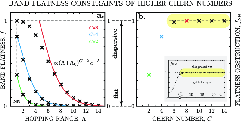
We show that the finite Chern number inevitably leads to constraints on the band flatness (Fig.1). We note that high $C$$=$$N$ in (8) can be attained in multiple ways. The simplest way is by having two poles of multiplicity $N$ each ²²2Double periodic meromorphic function cannot have less than two zeros, two poles counting multiplicity. This results into a higher Chern number $C_{2N}$$=$$2N$$\gg$$1$ restraining band flatness as $f$$\sim$$\Lambda^{C_{2N}-2}e^{-2ha\Lambda}$. To have a topological band, the wave function singularity must reside inside the BZ. This leads to the limitation $h$$\leq$$\pi/a$ (square lattice), or $ha$$\sim$$1$ independently of $a$ and lattice symmetries. The flatness parameter is

Thus we come to the conclusion that the Chern bands cannot be perfectly flat unless in the case of infinite hopping range $\Lambda$. This observation is consistent with Chen theorem (2014), stating that in the double-periodic system the perfectly flat Chern bands are accessible only for $\Lambda=\infty$ Chen et al. (2014).

Flat Chern bands with C=1.—Now we can relax some of the conditions imposed in Eqs. (9), (8) on the flat band wave function. This can be done in two ways: by relaxing double periodicity or by relaxing holomorphicity conditions. First, we can relax condition of double-periodicity, but still require the flat band state to be a function of $z$$=$$k_{x}$$+$$ik_{y}$. In this way we unlock all the odd Chern numbers in (8), including unitary $|C|=1$. In this case the contribution along the BZ boundary, which vanishes due to double-periodicity in (8), may itself contribute to the Chern number. Interestingly, we can go even further by canceling the remaining singularity(-ies) inside the BZ and producing an effective magnetic flux; in this case the Chern number is given purely by the circulation along the BZ boundary $\oint_{\gamma}\mathbf{A}d\mathbf{k}=2\pi C$ Zak (1989). This case corresponds to the continuum model of twisted bilayer graphene (TBG), which hosts perfectly flat Chern bands at the magic angle San-Jose et al. (2012); Tarnopolsky et al. (2019). Several authors has pointed out on the duality between the perfectly flat Chern bands in TBG and the lowest Landau level; we refer to Refs.San-Jose et al. (2012); Tarnopolsky et al. (2019); Popov and Milekhin (2021) for further details. In both cases we are dealing with effective magnetic fields which produce Berry curvature $F_{xy}\propto l_{B}^{2}$, flux $2\pi$ through effective Brillouin zone (MBZ) and a perfectly flat band in a certain limit. Following Qi (2011), without loss of generality we can consider asymptote $\mathcal{W}(x)\propto x^{n}e^{-x^{2}/2l_{B}^{2}}$. Thus for Landau Levels the flatness criterion (1) asymptotically reads

where we assume $a$$\ll$$l_{B}$. We see that the Landau levels are perfectly flat only in the nonlocal limit $\Lambda$$\gg$$l_{B}/a$$\to$$\infty$. Bringing this system on the tight-binding lattice (finite $a$, finite $\Lambda$) inevitably broadens the Landau levels for any finite $\Lambda$, see Refs.Hofstadter (1976); Kapit and Mueller (2010); Dong and Mueller (2020).

We can further relax the condition of holomorphicity, but keep the condition of double periodicity. This correspond to the Chern bands constructed from the pairs of Dirac points. A simplest construction is $C=1/2+1/2$ Chern band constructed from two Dirac cones carrying Chern number $|C|=1/2$ each. The total Chern number is integer since the Dirac nodes always come in pairs on the lattice. Since the normalized wave function associated with a (gapped) Dirac cone contains singularity of form $u(k)$$\sim$$(k-k_{*})^{-1/4}$, the Wannier asymptotics is of form $\mathcal{W}(x)$$\sim$$x^{-3/4}e^{-hx}$. Since we again have restriction $ha$$\sim$$1$, we arrive to the flatness criterion of form $f\sim\Lambda^{-3/2}e^{-\Lambda}$. Once again we cannot have a perfectly flat band at local tight binding. Note that we can also construct higher Chern number $C=N$ by taking at least $2N$ Dirac cones and melting them into a flattened band (a strategy proved to be fruitful in graphene multilayers). This case completes our discussion on flatness of Chern bands, since further dropping both the condition of periodicity and holomorphicity breaks down the concept of Chern number as an integer topological invariant on the tight-binding level.

Independently of the method the flat Chern band has been composed, it is safe to rewrite the flatness criterion as

Comparing criterion (13) with the $f_{0}$ criterion for trivial bands (7), we notice that criterion (13) is not reducible to the atomic insulator. This is because the Chern insulator and atomic insulator belong to different topological classes, and cannot be adiabatically connected Chiu et al. (2016).

Microscopic analysis and hopping range bounds.—We now look deeper into the microscopic details of topological constraints (Fig. 2). A representative parameter is the hopping range scale, defined for an isolated band as

For definiteness, we use the construction of higher-Chern flat band as in Eqs.(10-11). We observe numerically that $r_{\text{hop}}^{2}$ behaves monotonically with $\tilde{h}$$=$$ha$; for $ha$$\lesssim$$1$ we have $r_{\text{hop}}^{2}$$\sim$$1/\tilde{h}^{2}$; $r_{\text{hop}}^{2}$$\sim$$\,C$. To understand this asymptotics analytically, we replace sum with integrals in definition above, $r_{\text{hop}}^{2}$$\simeq$$h^{-2}I[p_{n}$$-$$1,2]/I[p_{n}$$-$$1,0]$, with $I[q,s]$$=$$\iint\limits_{0}^{\infty}dx_{1}dx_{2}(x_{1}x_{2})^{q}(x_{1}$$-$$x_{2})^{s}e^{-(x_{1}+x_{2})}$. We arrive to the analytical expression $r_{\text{hop}}^{2}$$=$$2\Gamma(p_{n}+1)/h^{2}\Gamma(p_{n})$. Since in this case $p_{n}$ are integers, we have $r_{\text{hop}}^{2}$$=$$2p_{n}/h^{2}$. Restoring connection between the poles and the Chern number as in Eq.(11), we obtain

The wave function singularity position $h$=$h_{\text{max}}$ results into the lower bound for hopping range (14). For the Chern bands, it is impossible to remove this singularity to infinity, thus $h_{\text{max}}$ is bounded from above. For a square lattice, the first estimate on $h_{\text{max}}$ gives as $\pi/a$. Independently of lattice symmetries, we can use $h_{\text{max}}a$$\sim$$1$, hence the lower bound for hopping range in case of topological bands scales as (Fig.2a)

This agrees with Ref.Jian et al. (2013). Note that the actual hopping range cutoff $\Lambda_{*}$ required to stabilize the band of desirable flatness $f_{*}$ with respect to next-order hoppings can be much higher than the lower bound (15) scaling as $\propto$$Ca$ (Fig.2b).

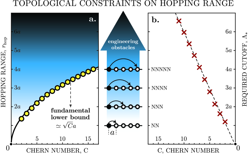
Bypassing higher Chern constraints.—We notice that the microscopic constraints of form (14),(15), which were derived assuming higher-order poles of multiplicity $N$$=$$C/2$, could be bypassed in the experiment. Instead, we can take (a physically reasonable number) $N$ of simple poles to construct $C$$=$$N$$\times$$C_{1}$ flat band using $C_{1}$$=$$1$. In this case $\mathcal{W}(x)$$\sim$$x^{C_{1}-1}e^{-hax}$, hence we need to replace $C$ with $C_{1}$ in (15), and the lower bound $\sqrt{C_{1}}$$a\sim a$ remains fixed on the lattice size for all the Chern numbers. Consider a thin film material (e.g. a monolayer or bilayer) with its band structure hosting a flat Chern band of unit $|C_{1}|$$=$$1$. We can stack $N$ such layers into a multilayer heterostructure, represented by matrix Hamiltonian $\mathcal{H}$ with monolayer Hamiltonians on the main diagonal and interlayer coupling terms placed on the diagonals just below and above. The topological invariant of this composition can be found through computing $C[\mathbb{G}]$$=$$\frac{1}{3!}\sum_{ijk}\epsilon_{ijk}\text{Tr}\,\mathbb{G}\partial_{i}\mathbb{G}^{-1}\mathbb{G}\partial_{j}\mathbb{G}^{-1}\mathbb{G}\partial_{k}\mathbb{G}^{-1},$ where $i,j,k$$=$$\omega$,$k_{x}$,$k_{y}$ and $\mathbb{G}=(\omega-\mathcal{H})^{-1}$ is matrix Green’s function Gurarie (2011). Consider a case of vanishingly weak interlayer interaction; in this case the Hamiltonian approximately factorizes into matrix tensor product. If the Chern number, associated with a single layer is $C_{1}$, the $N$ layers in this case give

This argument is expected to be valid when the weak interlayer interactions are switched on while preserving the finite gap; a similar algorithm was implemented by Trescher and Bergholtz Trescher and Bergholtz (2012). Importantly, the construction (16) does not obstruct the band flatness, i.e. the flat Chern bands can be constructed for any number of layers $N$. Clearly, this argument is also valid for constructing higher Chern numbers by bringing together $2n$ (gapped) Dirac cones in van der Waals multilayers for reaching $C$$=$$1,2,3...$ nearly flat Chern bands Zhang et al. (2019).

Conclusions.—To conclude, the new criterion for band flatness (1) allows us to derive two concise cases $f_{0}$$=$$e^{-ha\Lambda}$ for trivial bands and $f_{0}$$=$$\Lambda^{S[C]}e^{-F[\Lambda]}$ for topological bands of Chern number $C$. The criteria allows us to systematize the known classes of perfectly flat bands (Table I) as the fundamental building blocks for realistic nearly flat bands. The large Chern number presents an obstruction to the band flatness, which can be seen in e.g. in the required range $\propto$ $\sqrt{C}a$. The most feasible route for overcoming this obstruction is using multilayers for gluing together higher Chern numbers. We can hope that the strategy for building higher-$C$ bands with proposed pathways (16) shall become a route towards realizing elusive Kitaev $E_{8}$ state, a bosonic Quantum Hall phase which can be build on the $C$$=$$8n$ flat band Kitaev (2006).

$\bigodot$

Acknowledgements. The author thanks Bertrand Halperin, Subir Sachdev, Philip Kim, and Emil Bergholtz for enlightening discussions. This work was financed by the Branco Weiss Society in Science, ETH Zurich, through the research grant on flat bands, strong interactions and the SYK physics.

References

- Landau (1930) L. Landau, Zeitschrift für Physik 64, 629 (1930).
- Landau and Lifshitz (1977) L. D. Landau and E. M. Lifshitz, Quantum mechanics: non-relativistic theory (Pergamon Press, 1977).
- Haldane (2018) F. Haldane, Journal of Mathematical Physics 59, 081901 (2018).
- Kapit and Mueller (2010) E. Kapit and E. Mueller, Physical Review Letters 105, 215303 (2010).
- Miyahara et al. (2005) S. Miyahara, K. Kubo, H. Ono, Y. Shimomura, and N. Furukawa, Journal of the Physical Society of Japan 74, 1918 (2005).
- Maimaiti et al. (2017) W. Maimaiti, A. Andreanov, H. C. Park, O. Gendelman, and S. Flach, Physical Review B 95, 115135 (2017).
- Rhim and Yang (2019) J.-W. Rhim and B.-J. Yang, Phys. Rev. B 99, 045107 (2019).
- Trambly de Laissardière et al. (2010) G. Trambly de Laissardière, D. Mayou, and L. Magaud, Nano Letters 10, 804 (2010).
- Naik and Jain (2018) M. H. Naik and M. Jain, Physical Review Letters 121, 266401 (2018).
- Carr et al. (2020) S. Carr, C. Li, Z. Zhu, E. Kaxiras, S. Sachdev, and A. Kruchkov, Nano Letters 20, 3030 (2020).
- Cao et al. (2018) Y. Cao, V. Fatemi, S. Fang, K. Watanabe, T. Taniguchi, E. Kaxiras, and P. Jarillo-Herrero, Nature 556, 43 (2018).
- Yankowitz et al. (2019) M. Yankowitz, S. Chen, H. Polshyn, Y. Zhang, K. Watanabe, T. Taniguchi, D. Graf, A. F. Young, and C. R. Dean, Science 363, 1059 (2019).
- Park et al. (2021) J. M. Park, Y. Cao, K. Watanabe, T. Taniguchi, and P. Jarillo-Herrero, Nature 590, 249 (2021).
- Hao et al. (2021) Z. Hao, A. Zimmerman, P. Ledwith, E. Khalaf, D. H. Najafabadi, K. Watanabe, T. Taniguchi, A. Vishwanath, and P. Kim, Science 371, 1133 (2021).
- Neupert et al. (2011) T. Neupert, L. Santos, C. Chamon, and C. Mudry, Physical Review Letters 106, 236804 (2011).
- Tang et al. (2011) E. Tang, J.-W. Mei, and X.-G. Wen, Physical Review Letters 106, 236802 (2011).
- Sun et al. (2011) K. Sun, Z. Gu, H. Katsura, and S. D. Sarma, Physical Review Letters 106, 236803 (2011).
- Haldane (2011) F. Haldane, Physical Review Letters 107, 116801 (2011).
- Kitaev (2015) A. Kitaev, Talk at KITP, University of California, Santa Barbara (2015).
- Sachdev and Ye (1993) S. Sachdev and J. Ye, Physical Review Letters 70, 3339 (1993).
- Chen et al. (2018) A. Chen, R. Ilan, F. De Juan, D. Pikulin, and M. Franz, Physical Review Letters 121, 036403 (2018).
- Haldane (1988) F. D. M. Haldane, Physical Review Letters 61, 2015 (1988).
- Kohn (1959) W. Kohn, Physical Review 115, 809 (1959).
- He and Vanderbilt (2001) L. He and D. Vanderbilt, Physical Review Letters 86, 5341 (2001).
- Apostol (1951) T. M. Apostol, Pacific Journal of Mathematics 1, 161 (1951).
- Johnson (1974) B. Johnson, Pacific Journal of Mathematics 53, 189 (1974).
- Akhiezer (sian) N. I. Akhiezer, Elements of the theory of elliptic functions (American Mathematical Society, 1990; Gos.Tech.Izdat. 1948 [in Russian]).
- Jian et al. (2013) C.-M. Jian, Z.-C. Gu, and X.-L. Qi, Physica Status Solidi RRL 7, 154 (2013).
- Baum and Bott (1970) P. F. Baum and R. Bott, in Essays on Topology and related topics (Springer, 1970) pp. 29–47.
- Thouless (1984) D. Thouless, Journal of Physics C: Solid State Physics 17, L325 (1984).
- Po et al. (2018) H. C. Po, H. Watanabe, and A. Vishwanath, Phys. Rev. Lett. 121, 126402 (2018).
- Qi (2011) X.-L. Qi, Physical Review Letters 107, 126803 (2011).
- Note (1) Numerical analysis gives with .
- Note (2) Double periodic meromorphic function cannot have less than two zeros, two poles counting multiplicity.
- Chen et al. (2014) L. Chen, T. Mazaheri, A. Seidel, and X. Tang, Journal of Physics A 47, 152001 (2014).
- Zak (1989) J. Zak, Physical Review Letters 62, 2747 (1989).
- San-Jose et al. (2012) P. San-Jose, J. Gonzalez, and F. Guinea, Physical Review Letters 108, 216802 (2012).
- Tarnopolsky et al. (2019) G. Tarnopolsky, A. J. Kruchkov, and A. Vishwanath, Physical Review Letters 122, 106405 (2019).
- Popov and Milekhin (2021) F. K. Popov and A. Milekhin, Physical Review B 103, 155150 (2021).
- Hofstadter (1976) D. R. Hofstadter, Physical Review B 14, 2239 (1976).
- Dong and Mueller (2020) J. Dong and E. J. Mueller, Physical Review A 101, 013629 (2020).
- Chiu et al. (2016) C.-K. Chiu, J. C. Teo, A. P. Schnyder, and S. Ryu, Reviews of Modern Physics 88, 035005 (2016).
- Gurarie (2011) V. Gurarie, Physical Review B 83, 085426 (2011).
- Trescher and Bergholtz (2012) M. Trescher and E. J. Bergholtz, Physical Review B 86, 241111 (2012).
- Zhang et al. (2019) Y.-H. Zhang, D. Mao, Y. Cao, P. Jarillo-Herrero, and T. Senthil, Physical Review B 99, 075127 (2019).
- Roy (2014) R. Roy, Physical Review B 90, 165139 (2014).
- Jackson et al. (2015) T. S. Jackson, G. Möller, and R. Roy, Nature communications 6, 1 (2015).
- Claassen et al. (2015) M. Claassen, C. H. Lee, R. Thomale, X.-L. Qi, and T. P. Devereaux, Phys. Rev. Lett. 114, 236802 (2015).
- Note (3) The lowest Landau level automatically satisfies ; a delicate moment here is discussion of the higher Landau levels which at first glance violate this condition. However, since the wave functions of the higher Landau levels can be chosen holomorphic Haldane (2018); Chen and Biswas (2020), surprisingly this argument still holds.
- Chen and Biswas (2020) Y. Chen and R. R. Biswas, Physical Review B 102, 165313 (2020).
- Kitaev (2006) A. Kitaev, Annals of Physics 321, 2 (2006).