Ordinary Differential Equation-based CNN for Channel Extrapolation over RIS-assisted Communication

With the increasing demands for communication services, the number of connected devices continues to augment exponentially and new, blossoming service requirements pose more constraints on the network. At the same time, the increased power consumption and hardware cost remain key issues [1]. A recent technological breakthrough that holds the potential to overcome these technological bottlenecks is reconfigurable intelligent surface (RIS). It can be coated on any environmental object in a cost-effective manner, thereby facilitating the large scale deployment. Due to the physical characteristics of RIS, it can reflect incident electromagnetic waves, and adjust their amplitude and phase in a controlled manner. In other words, RIS can manipulate the communication environment in an intelligent way. Furthermore, the reflection elements of RIS usually work in a passive state, which makes RIS have low power consumption [2]. Hence, RIS is considered as a promising technology and attracts more and more attention.

Similar to the case of other communication systems [3], the acquisition of channel state information (CSI) is an important problem and has become a hot research topic in RIS-assisted communication systems. In [4], Ardah et al. designed a two-stage channel estimation framework with high resolution. In [5], the atomic norm minimization was resorted to implement the channel estimation over RIS-aided MIMO system in the millimeter wave frequency band.

All of the above works depend on the hypothetical statistical model. However, in the actual communication scenario, the radio scattering conditions change rapidly with time and are very complicated. This makes the traditional methods have some limitations [3]. With the development of the artificial intelligence, the application of deep learning (DL) in RIS-aided systems has attracted extensive attention. In [6], the authors adopted fully connected neural networks to estimate the RIS channel and detect the symbols. In [7], Elbir et al. designed a twin convolutional neural network (CNN) to estimate the direct and the cascaded channel in a RIS-aided communication system. However, due to the passive characteristics of RIS, the channels from the source to RIS and that from RIS to destination are coupled, and the size of the equivalent channel is in scale with the number of the RIS elements, which is usually large enough to accurately manipulate an incoming electromagnetic (EM) field. Thus, it would cost many pilot resource to directly achieve the equivalent channel of large size at destination. Thus, how to reduce the overhead of the channel estimation is an interesting topic over the RIS-aided network. Recently, Taha et al. used a small part of RIS elements to sub-sample the channels, and optimize the beamforming vector of RIS with the channel estimated at the selected elements [8].

In this paper, we further examine the channel compression over the physical space for RIS-aided communication. After selecting a fraction of the RIS elements, we achieve the equivalent channel formed by the source, the destination and the chosen RIS elements. Then, we extrapolate the channels to all elements from those estimated at chosen elements, where DL is adopted. Furthermore, inspired by the ordinary differential equation (ODE), we modify the structure of the cascaded CNN by adding cross-layer connections, namely introducing coefficients and linear calculations between the network layers. The proposed ODE-based CNN can obtain more accurate solutions, and its performance can be verified to be better than the cascaded CNN.

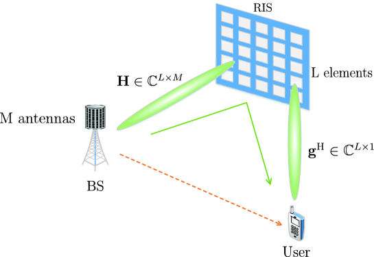
As shown in Fig. 1, let us consider an indoor scenario, where multiple-antenna base station (BS) communicates with a single-antenna user via RIS reflection. A BS is equipped with a uniform linear array (ULA) with $M$ antennas. RIS is in the form of a uniform planar array (UPA) and consists of $L=L_{h}L_{v}$ elements, where $L_{h}$ and $L_{v}$ separately denotes the sizes along the horizontal and vertical dimensions. Moreover, the orthogonal frequency division multiplexing (OFDM) scheme is adopted and the number of subcarriers is $K$. Since the indoor environment is easy to be blocked by objects or people, the direct channel between the BS and the user may be destroyed. Thus, we only consider the channel reflected by RIS, i.e., the cascaded channel, instead of the direct channel. Obviously, the cascaded channel consists of two parts: the link from the BS to the RIS, i.e., $\mathbf{H}\in\mathbb{C}^{L\times M}$, and that from the RIS to the user, i.e., $\mathbf{g^{\mathrm{H}}}\in\mathbb{C}^{L\times 1}$. The received signal at the $k$-th subcarrier of the user can be given as

where $\mathbf{\Psi}\in\mathbb{C}^{L\times L}$ is a diagonal matrix, i.e., $\mathbf{\Psi}=\text{diag}\{\beta_{1}\text{exp}(j\phi_{1}),\dots,\beta_{L}\text{exp}(j\phi_{L})\}$, $\mathbf{s}_{k}$ is the downlink $M\times 1$ transmitted signal at the $k$-th sub-carrier, and $n_{k}\sim\mathcal{CN}(0,\sigma_{n}^{2})$ is the addictive white Gaussian noise. Due to the lack of signal processing capability at RIS, $\boldsymbol{\Psi}$ is the same at different sub-carriers. Notice that $\phi_{i}$ in $\mathbf{\Psi}$ represents the phase shift introduced by each RIS element while $\beta_{i}$ controls this element’s on-off state, which will be described in the following. Moreover, the channel between BS and RIS at the $k$-th subcarrier is given by

where $h_{i,f_{c}}$ is the complex channel gain along the $i$-th scattering path at the carrier frequency $f_{c}$, $\tau_{h,i}$ is the time delay, and $\mathbf{a}_{r}(\phi_{h,i},\theta_{h,i})$, $\mathbf{a}_{t}(\psi_{h,i})$ are the spatial steering vectors, with $\phi_{h,i}$ and $\theta_{h,i}$ as the azimuth angle and elevation angle of the receiver, respectively, and $\psi_{h,i}$ as the angle of departure (AoD). Correspondingly, $\mathbf{a}_{r}(\phi_{h,i},\theta_{h,i})$ can be written as

where the $L_{v}\times 1$ vector $\mathbf{a}_{el}(\phi_{h,i})=[1,e^{-j2\pi\frac{d}{\lambda_{c}}\cos\phi_{h,i}},\dots,e^{-j2\pi\frac{d}{\lambda_{c}}(L_{v}-1)\cos\phi_{h,i}}]^{\mathrm{T}}$ and the $L_{h}\times 1$ vector $\mathbf{a}_{az}(\phi_{h,i},\theta_{h,i})=[1,e^{-j2\pi\frac{d}{\lambda_{c}}\sin\phi_{h,i}\cos\theta_{h,i}},\dots,e^{-j2\pi\frac{d}{\lambda_{c}}(L_{h}-1)\sin\phi_{h,i}\cos\theta_{h,i}}]^{\mathrm{T}}$. $\lambda_{c}$ is the carrier wavelength and $d$ denotes antenna spacing. Furthermore, $\otimes$ represents the Kronecker product operator and $[\cdot]^{\mathrm{T}}$ represents the transpose. Moreover, $\mathbf{a}_{t}(\psi_{h,i})$ can be given by

Correspondingly, the channel between the RIS and the user at the $k$-th subcarrier is

where the structure of $\mathbf{a}_{t}(\phi_{g,i},\theta_{g,i})$ is similar to that of $\mathbf{a}_{r}(\phi_{h,i},\theta_{h,i})$.

The cascaded channel matrix between BS and the user at the $k$-th subcarrier can be defined as $\mathbf{C}_{k}=\mathbf{G}_{k}\mathbf{H}_{k}$, where $\mathbf{G}_{k}=\mathrm{diag}\{\mathbf{g}_{k}\}$, and $\mathbf{C}_{k}$ has a size of $L\times M$. Then, let us define the $LM\times 1$ vector $\mathbf{c}_{k}=[\mathbf{c}_{k,1}^{\mathrm{T}},\dots,\mathbf{c}_{k,L}^{\mathrm{T}}]^{\mathrm{T}}$, where $\mathbf{c}_{k,i}$ represents the $i$-th column of $\mathbf{C}_{k}$. Within the RIS communication system, it is proved that the optimal $\boldsymbol{\Psi}$ is closely related with all the cascaded channels at $K$ subcarriers, i.e., $\mathbf{C}=[\mathbf{c}_{1},\mathbf{c}_{2},\dots,\mathbf{c}_{K}]$ [9]. Hence, our aim is to estimate $\mathbf{C}$.

In this section, we evaluate the channel extrapolation performance of ODE-based CNN through numerical simulation. We first describe the communication scenario and dataset source, and then show the parameters of the training network. Finally, we show the simulation results and explain the performance of our proposed network.

The scenario we consider is an indoor scene with user, BS and RIS. To generate this scenario, we resort to the indoor distributed massive MIMO scenario I1 of the DeepMIMO dataset, which is generated based on the Wireless InSite [14].

The ULA at BS has $4$ antennas, i.e., $M=4$, while the size of the RIS’s UPA is $8\times 8$, i.e., $L=64$. The carrier frequency of channel estimation is $2.4$ GHz. The OFDM signal bandwidth is set as $20$ MHz, while the number of subcarriers is $K=64$. The antenna spacing is $\frac{\lambda}{2}$, and the number of paths is $5$. Furthermore, the activated users are located from the $1$-st row to the $100$-th row. Each row contains $201$ users, and the total number of users is $20100$. The users are split in two parts, i.e., the training and the test groups, according to the ratio $4:1$. The sampling rate $r=\frac{N}{L}$ is separately set as $\frac{1}{2},\frac{1}{4},\frac{1}{8}$ and $\frac{1}{16}$.

In the simulations, we adopt three network structures for comparison, i.e., the ODE-RK3 structure formed by some RK3-Blocks, the ODE-LF structure containing several LF-Blocks and the cascaded CNN network. For fairness, all CNNs have $26$ layers and the same number of parameters. The ODE-based network contains $4$ RK3-Blocks or LF-Blocks (each block consists of $6$ convolutional layers), a head convolutional layer and a tail convolutional layer. Considering ODE-RK3 structure as an example, we list the layer parameters of the CNN in TABLE I. Specially, in the hidden layers, the number of neurons is $128$, and $\mathrm{ReLU}$ is adopted as the activation function, i.e., $\mathrm{ReLU}(x)=\max(x,0)$. The kernel size of the first convolutional layer is $5\times 5$, and that of the remainder convolutional layers is set as $3\times 3$. The learning rate $\eta$ is initialized as $0.0005$ and decreases with increased iteration times. Specifically, after $40$ iterations, the learning rate reduces by $20\%$ for every $10$ epochs.

TABLE II shows the performance of different network structures. It can be noted that the proposed ODE CNN is always superior to the cascaded CNN network, and this gain enhances with the increase of the sampling rate $r$. The RK3 structure with three-order performs better than the third-order LF structure. When sampling rates are $\frac{1}{2}$ and $\frac{1}{4}$, the ODE-RK3 structure can achieve satisfactory results. Furthermore, in terms of channel extrapolation normalized MSE (NMSE), the ODE-RK3 network at $r=\frac{1}{4}$ performs better than the CNN network at $r=\frac{1}{2}$, which means that the length of the pilot for the sub-sampled channel $\widetilde{\mathbf{C}}$ estimation can be reduced through introducing the ODE structure. If the compression ratio is relatively low, such as $r=\frac{1}{16}$, the performance of the ODE-based CNN is not significantly better than that of the cascaded CNN due to the reduced raw input information for the channel extrapolation.

Fig. 3 depicts the curves of NMSE with respect to the number of epochs. Two structures (the ODE-RK3 and cascaded CNN structures) and two sample rates ($\frac{1}{4}$ and $\frac{1}{8}$) are considered here. It can be seen that with the increase of iteration time, all the NMSE curves present a downward trend and reach the stable levels after $115$ epochs. Furthermore, for a given sampling rate, the NMSEs of the ODE-based CNN are always lower than those of the cascaded CNN. Fig. 4 depicts the training loss of different CNN structures versus epochs. It can be checked from Fig. 4 that, with fixed rate $r$, the training loss in the ODE-RK3 network decreases faster than that in the cascaded CNN network, which means that the ODE-based network can be trained more quickly than CNN.

So far, we considered the channel extrapolation at the same frequency band. However, our proposed scheme can still be used for the case with frequency difference. In actual systems, such as the frequency division duplexing system, the uplink and downlink channels operate in different frequency bands. Fig. 5 shows the performance of the ODE-RK3 and the cascaded CNN structures under different frequency gaps. As can be seen from Fig. 5, both ODE-RK3 and CNN structures are affected by the frequency gaps. As the frequency difference increases, the NMSE of channel extrapolation slightly augments. It is worth noting that the ODE-RK3 structure always performs better than cascaded CNN, which proves the stability and effectiveness of the proposed ODE-based CNN.

In this paper, we have examined a RIS-assisted MIMO communication system, and designed an ODE-based CNN to extrapolate the cascaded channel. In our scheme, only part of the full CSI is needed. Hence, some of the RIS elements could be turned off through spatial sampling, which greatly reduces the length of the pilot sequence in the channel estimation phase and improves the resource utilization. Simulation results have demonstrated that the proposed extrapolation scheme can effectively compress the large-scale RIS channel over the physical space. Moreover, the ODE-based structure can speed up the convergence and improve the performance of the cascaded CNN.

References

- [1] F. Rusek, D. Persson, B. K. Lau, E. G. Larsson, T. L. Marzetta, O. Edfors, and F. Tufvesson, “Scaling up MIMO: Opportunities and challenges with very large arrays,” IEEE Signal Process. Mag., vol. 30, no. 1, pp. 40–60, Jan. 2013.
- [2] W. Yan, X. Yuan, Z. He, and X. Kuai, “Passive beamforming and information transfer design for reconfigurable intelligent surfaces aided multiuser MIMO systems,” IEEE J. Sel. Areas Commun., pp. 1–1, 2020.
- [3] J. Ma, S. Zhang, H. Li, F. Gao, and S. Jin, “Sparse Bayesian learning for the time-varying massive MIMO channels: Acquisition and tracking,” IEEE Trans. Commun., vol. 67, no. 3, pp. 1925–1938, Mar. 2019.
- [4] K. Ardah, S. Gherekhloo, A. L. F. de Almeida, and M. Haardt, “TRICE: An efficient channel estimation framework for RIS-aided MIMO communications,” arXiv:2008.09499, 2020. [Online]. Available: https://arxiv.org/abs/2008.09499.
- [5] J. He, H. Wymeersch, and M. Juntti, “Channel estimation for RIS-aided mmWave MIMO systems via atomic norm minimization,” arXiv:2007.08158, 2020. [Online]. Available: https://arxiv.org/abs/2007.08158.
- [6] S. Khan, K. S Khan, N. Haider, and S. Y. Shin, “Deep-learning-aided detection for reconfigurable intelligent surfaces,” arXiv:1910.09136, 2020. [Online]. Available: https://arxiv.org/abs/1910.09136.
- [7] A. M. Elbir, A. Papazafeiropoulos, P. Kourtessis and S. Chatzinotas, “Deep channel learning for large intelligent surfaces aided mm-wave massive MIMO systems,” IEEE Wireless Commun. Lett., vol. 9, no. 9, pp. 1447-1451, Sept. 2020.
- [8] A. Taha, M. Alrabeiah, and A. Alkhateeb, “Enabling large intelligent surfaces with compressive sensing and deep learning,” arXiv:1904.10136v2, 2019. [Online]. Available: https://arxiv.org/abs/1904.10136v2.
- [9] S. Lin, B. Zheng, G. C. Alexandropoulos, M. Wen, M. Di Renzo, and F. Chen, “Reconfigurable intelligent surfaces with reflection pattern modulation: Beamforming design and performance analysis,” IEEE Wireless Commun. Lett., pp. 1-1, Oct. 2020.
- [10] K. He, X. Zhang, S. Ren, and J. Sun, “Deep residual learning for image recognition,” in Proc. IEEE Conference on Computer Vision and Pattern Recognition, Las Vegas, NV, pp. 770-778, Dec. 2016.
- [11] R. T. Q. Chen, Y. Rubanova, J. Bettencourt, and D. Duvenaud, “Neural ordinary differential equations,” arXiv:1806.07366v5, 2019. [Online]. Available: https://arxiv.org/abs/1806.07366.
- [12] X. He, Z. Mo, P. Wang, Y. Liu, M. Yang, and J. Cheng, “ODE-inspired network design for single image super-resolution,” in Proc. IEEE Conference on Computer Vision and Pattern Recognition, Long Beach, CA, pp. 1732-1741, Jun. 2019.
- [13] O. P. Kingma and J. Ba, “ADAM: A method for stochastic optimization,” arXiv:1412.6980, 2014, [Online]. Available: https://arxiv.org/abs/1412.6980
- [14] A. Alkhateeb, “DeepMIMO: A generic deep learning dataset for millimeter wave and massive MIMO applications,” in Proc. Information Theory and Applications Workshop (ITA), San Diego, CA, pp. 1-8, Feb. 2019.