Ordering for Non-Replacement SGD

Yuetong Xu and Baharan Mirzasoleiman

Abstract

One approach for reducing run time and improving efficiency of machine learning is to reduce the convergence rate of the optimization algorithm used. Shuffling is an algorithm technique that is widely used in machine learning, but it only started to gain attention theoretically in recent years. With different convergence rates developed for random shuffling and incremental gradient descent, we seek to find an ordering that can improve the convergence rates for the non-replacement form of the algorithm. Based on existing bounds of the distance between the optimal and current iterate, we derive an upper bound that is dependent on the gradients at the beginning of the epoch. Through analysis of the bound, we are able to develop optimal orderings for constant and decreasing step sizes for strongly convex and convex functions. We further test and verify our results through experiments on synthesis and real data sets. In addition, we are able to combine the ordering with mini-batch and further apply it to more complex neural networks, which show promising results.

1 Introduction

Throughout this paper we consider the minimization of the finite sum additive cost function with the update function of the form:

F(x)=\frac{1}{n}\cdot\sum_{i=1}^{n}f_{i}(x)\quad,\quad x_{i}=x_{i-1}-\alpha\nabla f_{i}(x_{i-1}).

(1)

Where the component functions $f_{i}$ are all convex if not strongly convex. This model is standard for learning from $n$ data examples, where $f_{i}$ represent the loss with respect to data sample $i$ . The data examples can be ordered by random or by specific permutation. In standard SGD and Random Shuffling (SGD without resampling), the algorithms randomize the order the data examples are processed and hence how the iterate is updated. $\alpha$ represent the learning rate or step size. In practice, algorithms apply decreasing learning rate for better convergence.

Only in recent years Shuffling, algorithms without replacement, started to attract attention of scholars in the field though in practice such algorithms are largely applied instead of SGD for optimization problems. It is already shown that Random Shuffling converges faster than SGD after finite epochs for strongly convex cases ([44]). [82] presented an upper bound for the distance between algorithm iterate and the optimal for incremental gradient descent (gradient descent with specific ordering) which establishes a basis for our analysis. The distance between the iterate and optimal is the error of the algorithm which we try to minimize. Hence by improving this distance, we can further optimize the algorithm.

For large scale machine learning, the size of the data can result in long run time and convergence time. One way to improve the efficiency of learning is to improve the convergence rate of the algorithms used. Stochastic gradient descent and Random Shuffling are one of the widely applied algorithms for large scale machine learning. In this paper, we seek to find an optimal ordering that can improve the convergence of the non-replacement algorithm.

In our analysis, we utilize the inherent properties of convex and strongly convex functions to develop a tighter upper bound whose value is dependent on the gradient values. From the bound we reach the following conclusions: For strongly convex function $f_{i}$ s, in which the functions are and Lipschitz continuous $f_{i}$ s with Lipschitz constant $L$ and bounded gradients with $M$ , if our initial $x_{0}$ is sufficiently close to the optimal and with initial step size $\alpha<\frac{1}{LGM}$ , then

•

for decreasing step size, ordering by decreasing initial gradient would result in the fastest convergence.
•

for constant step size, random ordering, ordering by decreasing gradient norm, ordering by increasing gradient norm all result in the same convergence rate.

From convex functions, with the same conditions, the results of regarding the ordering is the same.

We confirm our theoretical results through experiments on synthetic and real data sets including Iris data set and Boston Housing data set. By comparing the loss values for random ordering, decreasing gradient ordering, and increasing gradient ordering, we observed that the relationship stated above is indeed valid. We test the influence of the initial value of $x$ on the convergence in which if $x_{0}$ is close enough to the optimal $x^{*}$ , decreasing ordering is best. We further expand our results to more complex neural networks and mini-batch algorithms through experiments on MNIST data set, Fashion MNIST data set, and CIFAR data sets.

2 Related Works

Gradient Descent methods have been long studied and applied in research. Various studies have attempted to improve the convergence of SGD upon stochastic gradient descent by ordering based on average gradient error ([67]), ordering based on gradient bounds ([111]), ordering based on gradient error ([78]), and weighting samples by gradients ([3]). Others have approached the issue by decreasing batch size and prioritizing important data, e.g. by training on top $q$ samples from the batch with greatest loss ([54]), resampling a smaller batch for training based on pre-sampled data distribution ([52]), and training on data with smallest loss in the set ([103]).

In contrast to the existing volume of studies on SGD, Shuffling, the non-replacement version of SGD only started to gain attention recently. Large portion of results mostly focus on comparing Shuffling methods with SGD. [105] provided theoretical support that in worst case scenario, shuffling will not be significantly worse than SGD. [102] proved the optimization error decays with $O(\frac{1}{k})$ for SGD with replacement, while it is $O(\frac{1}{k^{2}})$ for SGD without replacement for sufficiently large k. [44] proved random shuffling could achieve better worst case convergence rates for all scenarios. In addition, many papers focus purely on theoretical guarantees on convergence rates of various shuffling methods. [82] proved the convergence rates of the Incremental Subgradient Methods which contain an upper bound for the distance between algorithm iterate and the optimal. [43] proposed a de-biased shuffling method which takes on averages of iterates with convergence rate of $O(\frac{1}{k^{2}})$ . [40] proved shuffling has convergence rate of $O(\frac{1}{k^{2}})$ . [90] proposed a unified convergence analysis of various shuffling methods in which randomized reshuffling is $O(\frac{1}{nT^{2}})$ with general case being $O(\frac{1}{T^{2}})$ . [96] provided a convergence rate of $O(\frac{1}{T^{2}}+\frac{n^{2}}{T^{3}})$ for quadratic functions and a lower bound of $\omega(\frac{n}{T^{2}})$ for strongly convex functions composed of summation of smooth functions. [77] further investigated on convergence behavior of random shuffling, shuffle once, and incremental gradient descent. [86] focused on methods with reweighting the sampling distribution.

Our paper is unique from existing work as it seeks to find a deterministic ordering of examples at every epoch that can improve the convergence of non-replacement SGD through providing theoretical and empirical evidence. Our permutation utilizes the gradient properties of the training data. It differs from related work in SGD not only from the non-replacement setting, but also that we derive a concrete permutation based on gradient value. It distinguishes from [54] in that our permutation results in a ordering of that can applied to full data while their result only samples the top $q$ data points of each batch with no specified order.

3 Optimal Ordering

The loss function we minimize is $F(x)=\frac{1}{n}\cdot\sum_{i=1}^{n}f_{i}(x)$ , where each $f_{i}$ is smooth and convex if not strongly convex. For this paper we will focus on the non-replacement version of SGD in which we would update each step as $x_{i,k}=x_{i-1,k}-\alpha_{i,k}\nabla f_{\sigma_{k}(i)}(x_{i-1,k})$ , where $x_{i,k}$ denote the iterated value at $i^{th}$ iteration of $k^{th}$ epoch, $\alpha_{i,k}$ denotes the step size at the corresponding iterate, $\nabla f$ denotes the sub-gradient at the corresponding iterate, and $\sigma_{k}(i)$ denote the permutation of the data values at epoch k. For simplicity, in the following content we would not explicitly write out $\sigma_{k}(i)$ in our equation and $x_{k}$ will denote the first point at epoch $k$ i.e. $x_{0,k}$ .

Assumption 1.

In this paper, we further assume there is a bound on the norm of the gradient of $f_{i}$ . (Denote as $C_{i}$ ).

||\nabla f_{i}(x)||\leq C_{i}\quad\forall x

(2)

Next, we provide near-optimal orderings for minimizing strongly convex and convex functions.

3.1 Strongly Convex Functions

Lemma 1.

For different $f_{i}$ s which are strongly convex or convex at the same iterate x, the larger $||\nabla f_{i}(x)^{T}||$ , the larger the upper bound for $f_{i}(x)-f_{i}(x^{*})$ , where $x^{*}$ denote the optimal point we seek to obtain. (The proof can be found in Appendix 6.1.)

Furthermore, by property of strongly convex function, for $\forall x$

f(x-A)\geq f(x)+\nabla f(x)^{T}(-A)+\mu^{2}||x-A||^{2}=f(x)-\nabla f(x)^{T}(A)+\mu^{2}||x-A||^{2}

(3)

where $\mu>0$ is the strongly convex constant.

For strongly convex functions, we obtain the permutation by observing the bound on distance between initial point of the epoch and the optimal solution, i.e. $||x_{k}-x^{*}||^{2}$ . By using existing bound from [82] and the existence of the lower bound of the strongly convex functions (Eq3), we are able to further tighten the upper bound on the distance by ordering the data points in a specific order. For strongly convex case, we would consider 2 scenarios: decreasing step size per iteration and constant step size.

Intuitively, for decreasing step size, if we wish to converge faster, we would need to have the algorithm approximate Gradient Descent as close as possible, which in turn suggests having larger gradients in the beginning of the epoch to pair with the relative larger values of the step sizes. On the other hand, if we assume the sub-gradient we obtain in the algorithm is very close to the actual value in gradient descent (since we are sufficiently close to the optimal), then no matter how we order the data points, with the same step size we would update the iterate with same amount after an epoch.

Theorem 1 (Strongly convex with decreasing step size per iteration).

For strongly convex functions $f_{i}$ that are differentiable, with bounded gradients, and with strongly convex constant $m_{i}$ , ordering by decreasing value of norm of gradient $M_{i}$ at the beginning of every epoch provides a tighter upper bound for $||x_{k+1}-x^{*}||$ , which is

\begin{array}[]{l@{}l}||x_{k+1}-x^{*}||^{2}\leq||x_{k}-x^{*}||^{2}-2||x_{k}-x^{*}||\sum_{i=1}^{n}\alpha_{i,k}||M_{i}||+\alpha_{k}^{2}\left(2\sum_{i=1}^{n-1}[(n-i)C_{i}^{2}]+\sum_{i=1}^{n}C_{i}^{2}\right)\\ \qquad\qquad\qquad\qquad\qquad\qquad-\alpha_{k}^{2}\alpha_{k+1}\sum_{i=1}^{n-1}(n-i)m_{i}\cdot max{(||M_{i}||,||M_{i}^{{}^{\prime}}||)}^{2}+n\alpha_{k}\cdot\epsilon_{k}\end{array}

(4)

In the equation, n denotes the total number of data samples, $\alpha$ representing the learning rate, and $\epsilon$ being a small constant. Since $\alpha$ is small, to minimize the bound on the difference with the optimal, we have to maximize the term of with $\alpha$ in first power, i.e. $\sum_{i=1}^{n}\alpha_{i,k}||M_{i}||$ . With decreasing step size, this suggest ordering by decreasing value of norm of gradients.

Theorem 2 (Strongly convex with constant step size).

For strongly convex functions $f_{i}$ that are differentiable, with bounded gradients, and with strongly convex constant $m_{i}$ , random ordering, ordering by decreasing gradient norm, ordering by increasing gradient norm generate the same upper bound for $||x_{k+1}-x^{*}||$ which is

\begin{array}[]{l@{}l}||x_{k+1}-x^{*}||^{2}\leq||x_{k}-x^{*}||^{2}-2\alpha||x_{k}-x^{*}||\sum_{i=1}^{n}||M_{i}||+\alpha^{2}\left(2\sum_{i=1}^{n-1}[(n-i)C_{i}^{2}]+\sum_{i=1}^{n}C_{i}^{2}\right)\\ \hskip 128.0374pt-\alpha^{3}\sum_{i=1}^{n-1}(n-i)m_{i}\cdot max{(||M_{i}||,||M_{i}^{{}^{\prime}}||)}^{2}+n\alpha\cdot\epsilon_{k}\end{array}

(5)

Similar as previous theorem, n denotes total samples, $\alpha$ denotes learning rate, and $\epsilon$ is a small constant. Since $\alpha$ is small and constant, the only value that can influence the upper bound is $\sum_{i=1}^{n}||M_{i}||$ . However, the sum of initial gradients would be the same if we start training from the same state, and hence the three orderings results the same upper bound.

The proof of the theorems can be found in the Appendix 6.

3.2 Convex Functions

Following the result of Lemma 1, for convex function, for $\forall x$

f(x-A)\geq f(x)+\nabla f(x)^{T}(-A)=f(x)-\nabla f(x)^{T}(A)

(6)

With this property, we can derive the following:

\begin{array}[]{l@{}l}f_{n}(x_{0,k}-\sum_{i=1}^{n-1}\alpha_{i,k}M_{i}^{{}^{\prime}})-f_{n}(x^{*})&\geq f_{n}(x_{0,k})-\nabla f_{n}(x_{0,k})^{T}(\sum_{i=1}^{n-1}\alpha_{i,k}M_{i}^{{}^{\prime}})-f_{n}(x^{*})\\ &{}\geq[f_{n}(x_{0,k})-f_{n}(x^{*})]-\sum_{i=1}^{n-1}\alpha_{i,k}\max{(||M_{i}||,||M_{i}^{{}^{\prime}}||)}^{2}\\ \end{array}

(7)

Following the logic for strongly convex loss function, the result about ordering the examples by the sub-gradient value at the beginning of the epoch also holds for convex loss functions.

Theorem 3 (Convex with decreasing step size per iteration).

For convex functions $f_{i}$ that are differentiable with bounded gradients, ordering by decreasing value of norm of gradient $M_{i}$ at beginning of every epoch provides a tighter upper bound for $||x_{k+1}-x^{*}||$ which is

\begin{array}[]{l@{}l}||x_{k+1}-x^{*}||^{2}\leq||x_{k}-x^{*}||^{2}-2||x_{k}-x^{*}||\sum_{i=1}^{n}\alpha_{i,k}||M_{i}||\\ \hskip 128.0374pt+\alpha_{k}^{2}\left(2\sum_{i=1}^{n-1}[(n-i)C_{i}^{2}]+\sum_{i=1}^{n}C_{i}^{2}\right)+n\alpha_{k}\cdot\epsilon_{k}\end{array}

(8)

Similar as the strongly convex case, with small learning rate $\alpha$ , to minimize the upper bound we need to maximize the term $\sum_{i=1}^{n}\alpha_{i,k}||M_{i}||$ . With decreasing step size, this implies ordering by decreasing gradient norm so the larger $||M_{i}||$ are paired with the larger $\alpha_{i,k}$ .

Theorem 4 (Convex with constant step size).

For convex functions $f_{i}$ that are differentiable with bounded gradients, random ordering, ordering by decreasing gradient norm, ordering by increasing gradient norm generate the same upper bound for $||x_{k+1}-x^{*}||$ which is

\begin{array}[]{l@{}l}||x_{k+1}-x^{*}||^{2}\leq||x_{k}-x^{*}||^{2}-2\alpha||x_{k}-x^{*}||\sum_{i=1}^{n}||M_{i}||\\ \hskip 128.0374pt+\alpha^{2}\left(2\sum_{i=1}^{n-1}[(n-i)C_{i}^{2}]+\sum_{i=1}^{n}C_{i}^{2}\right)+n\alpha\cdot\epsilon_{k}\end{array}

(9)

With constant step size and small step size $\alpha$ , the only term that can significantly change the upper bound is $\sum_{i=1}^{n}||M_{i}||$ . However, starting at the same state, the summation of gradient norms at beginning of the epoch is the same for the three orderings being compared. Therefore, the upper bound would be the same for the three orderings.

The proof of the theorems could be found in the Appendix 6.2. The direct result of these theorems is the following algorithm 1.

Algorithm 1 Full Data Ordering

step size

\alpha

, number of iterations T, initial weights

w_{0}

Construct gradient array G of size n

for t = 0, 1, …, T do

for i = 0, 1, …, n do

G[i]=||\nabla f(w_{T\cdot n+i};D[i])||

\triangleright

Calculate gradient norm

end for

Sort data points within sorted based on decreasing gradient norm, denote

\sigma_{T}

for i = 0, 1, …, n do

Update the model parameters:

w_{T\cdot n+i+1}\leftarrow w_{T\cdot n+i}-\alpha\nabla f(w_{T\cdot n+i};x(\sigma_{T}(i)))

end for

3.3 Ordering with Data Selection

In this algorithm, we split the data points into small batches of size S and iterate over q samples within each batch. Similar to decreasing ordering for full data, we can maximize $\sum_{i=1}^{n}\alpha_{i,k}||M_{i}||$ within each batch. Within batches, we select examples with largest gradients. If we assume $||M_{N\cdot S+{q+1}}||<||M_{(N+1)\cdot S+{1}}||$ (N: number of batches ran, S: size of each batch, q: the amount of sample we train on in each batch), then comparing continuing training on $q+1$ sample in $(N+1)$ th mini-batch and directing start training on $(N+2)$ th mini-batch results $\alpha_{N\cdot S+{q+1},k}||M_{N\cdot S+{q+1}}||<\alpha_{N\cdot S+{q+1},k}||M_{(N+1)\cdot S+{1}}||$ . Similar results follows for all points in the batch after the top q iterates with largest gradient norm.

For decreasing step size, with our algorithm, the iterates with large $||M_{i}||$ in the following batch will have a larger corresponding $\alpha_{i,k}$ , maximizing $\sum_{i=1}^{\frac{n}{S}\cdot q}\alpha_{i,k}||M_{i}||$ . For constant step size, since we assume the neglected data have a small gradient, the difference between neglecting and not neglecting the data will be small.

Algorithm 2 Ordering With Data Selection

step size

\alpha

, number of iterations T, initial weights

w_{0}

Construct data set into batches (B[i]s) of size S

Construct gradient array G of size S

for t = 0, 1, …, T do

for i = 0, 1, …, n do

for j = 0, 1, …, S do

\triangleright

Calculate gradient norm

G[i][j]=||\nabla f(w_{T\cdot n\cdot S+i\cdot S};B[i][j])||

\triangleright

B[i][j] denote the

j^{th}

point in batch i.

end for

Sort data points within B[i] sorted based on decreasing gradient norm, denote

\sigma_{T,i}

for j = 0, 1, …, S do

\triangleright

Update model parameters

w_{T\cdot n\cdot S+i\cdot S+j+1}\leftarrow w_{T\cdot n\cdot S+i\cdot S+j}-\alpha\nabla f(w_{T\cdot n\cdot S+i\cdot S+j};x(\sigma_{T,i}(j)))

end for

3.4 Ordering with Mini-Batch SGD

In addition to the ordering proposed above, we combine our ordering with mini-batch algorithm, which is a more efficient way of training ([54]), to apply to large data sets which SGD cannot be utilized. Two algorithms result from this combination: sorting before mini-batch and sorting within mini-batch.

For sorting before mini-batch, we directly combine our ordering to the mini-batch. In every epoch, we first order the data based on decreasing gradient ordering. Then we construct a balanced data set from the ordered data, in which each mini-batch contain equal number of data from each class if data is categorical. Following the construction, we run mini-batch algorithm on the resultant data set. We can control the size of data iterated by setting the mini-batch size to q instead of S if needed. Since we have sorted the data, the skipped data points will be the ones with small gradient norm. Hence with decreasing step size, the skipped data will have minimal effect on the model.

Algorithm 3 Sorting Before Mini-Batch

step size

\alpha

, number of iterations T, initial weights

w_{0}

for t = 0, 1, …, T do

Construct gradient array G of size nS

for k = 0, 1, …, nS do

\triangleright

Denote the data set as D, size nS.

G[k]=||\nabla f(w_{T*n};D[k])||

\triangleright

Calculate gradient norm

end for

Sort data points within D based on decreasing gradient norm, denote

\sigma_{T}

Construct balanced mini-batches from the ordered data.

for i = 0, 1, …, n do

Update the model parameters:

w_{T\cdot n+i+1}\leftarrow w_{T\cdot n+i}-\alpha\frac{1}{S}\sum_{j=0}^{S}\nabla f(w_{T\cdot n+i};x(\sigma_{T,i}(j)))

end for

Regarding sorting within mini-batch, instead of evaluating over the entire mini-batch (size $S$ ), within each mini-batch the top $q$ examples with largest gradients sorted in decreasing order are evaluated. The algorithm will calculate the gradients at beginning of each mini-batch, resulting in a finer gradient estimate for the entire batch.

Algorithm 4 Sorting Within Mini-Batch

step size

\alpha

, number of iterations T, initial weights

w_{0}

Construct data set into batches (B[i]s) of size S

Construct gradient array G of size S

\triangleright

B[i][j] denote the

j^{th}

point in batch i.

for t = 0, 1, …, T do

for i = 0, 1, …, n do

for j = 0, 1, …, S do

G[i][j]=||\nabla f(w_{T\cdot n+i\cdot S};B[i][j])||

\triangleright

Calculate gradient norm

end for

Sort data points within B[i] sorted based on decreasing gradient norm, denote

\sigma_{T,i}

Update the model parameters:

w_{T\cdot n+i+1}\leftarrow w_{T\cdot n+i}-\alpha\frac{1}{S}\sum_{j=0}^{S}\nabla f(w_{T\cdot n+i};x(\sigma_{T,i}(j)))

end for

Sorting within mini-batch is a more direct application of our result, but for large data sets, the calculation can be costly if the model needs to update and sort every mini-batch. Thus, for large data sets, sorting before mini-batch is a more practical and efficient way of training.

4 Data from Experiments

We further test our algorithm on synthetic data sets and real data sets to compare the loss function value for three ordering: random ordering, decreasing gradient norm, increasing gradient. For each ordering norm, we generate the corresponding permutation at the beginning of each epoch and visit the data points based on the ordering.

4.1 Synthetic Data

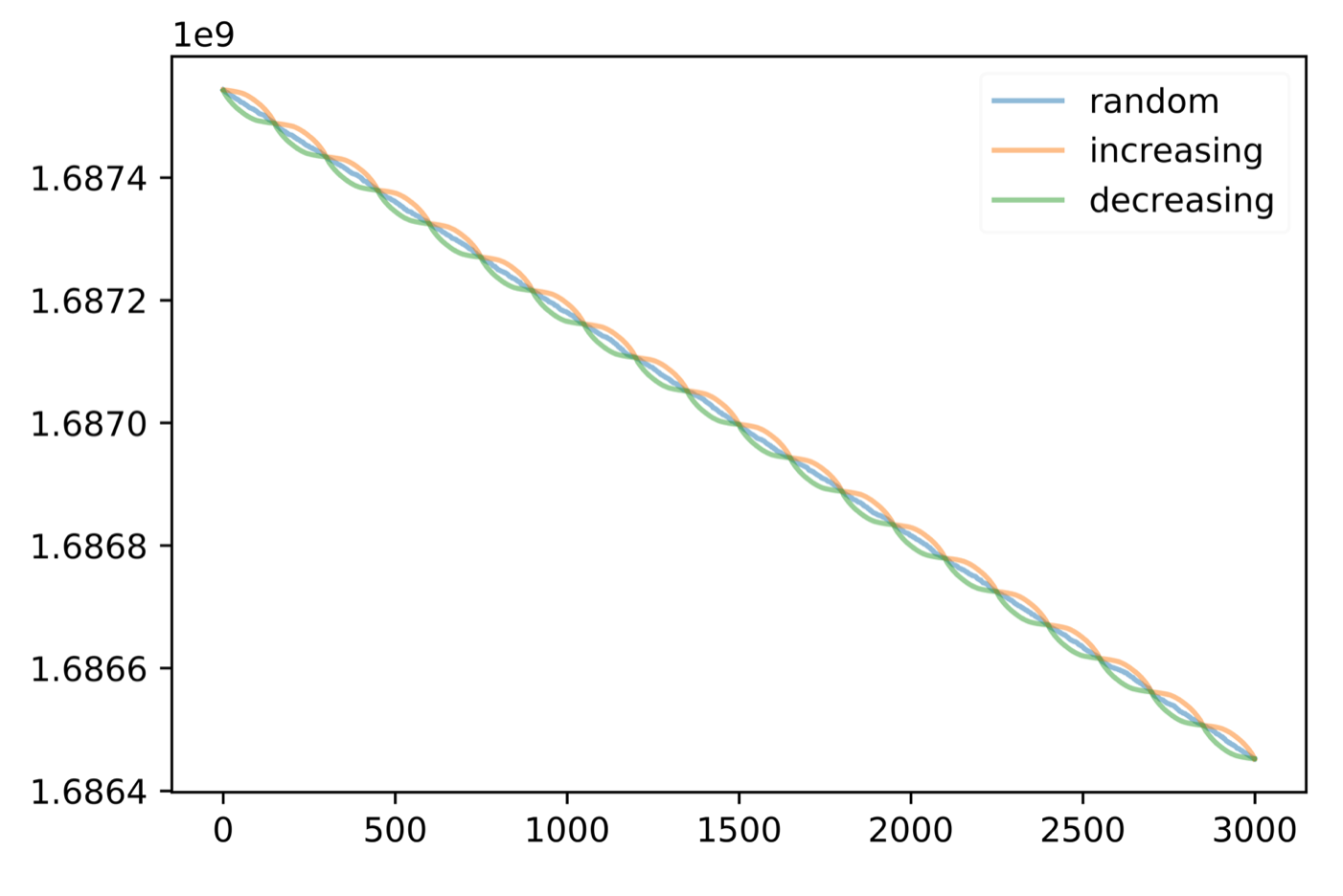
For the synthetic data, we randomly generate 32 vectors in $\mathbbm{R}^{2}$ with value in the range of [-10, 10]. The initial step size used for this case is $10^{-4}$ . The loss function is defined as $F=\sum_{i=1}^{m}||x-x^{*}||^{4}_{4}+||x-x^{*}||^{2}_{2}$ . The following graphs plot loss vs iteration for constant step size, decreasing step size per iteration, and decreasing step size per epoch correspondingly.

Refer to caption — (a) constant step size

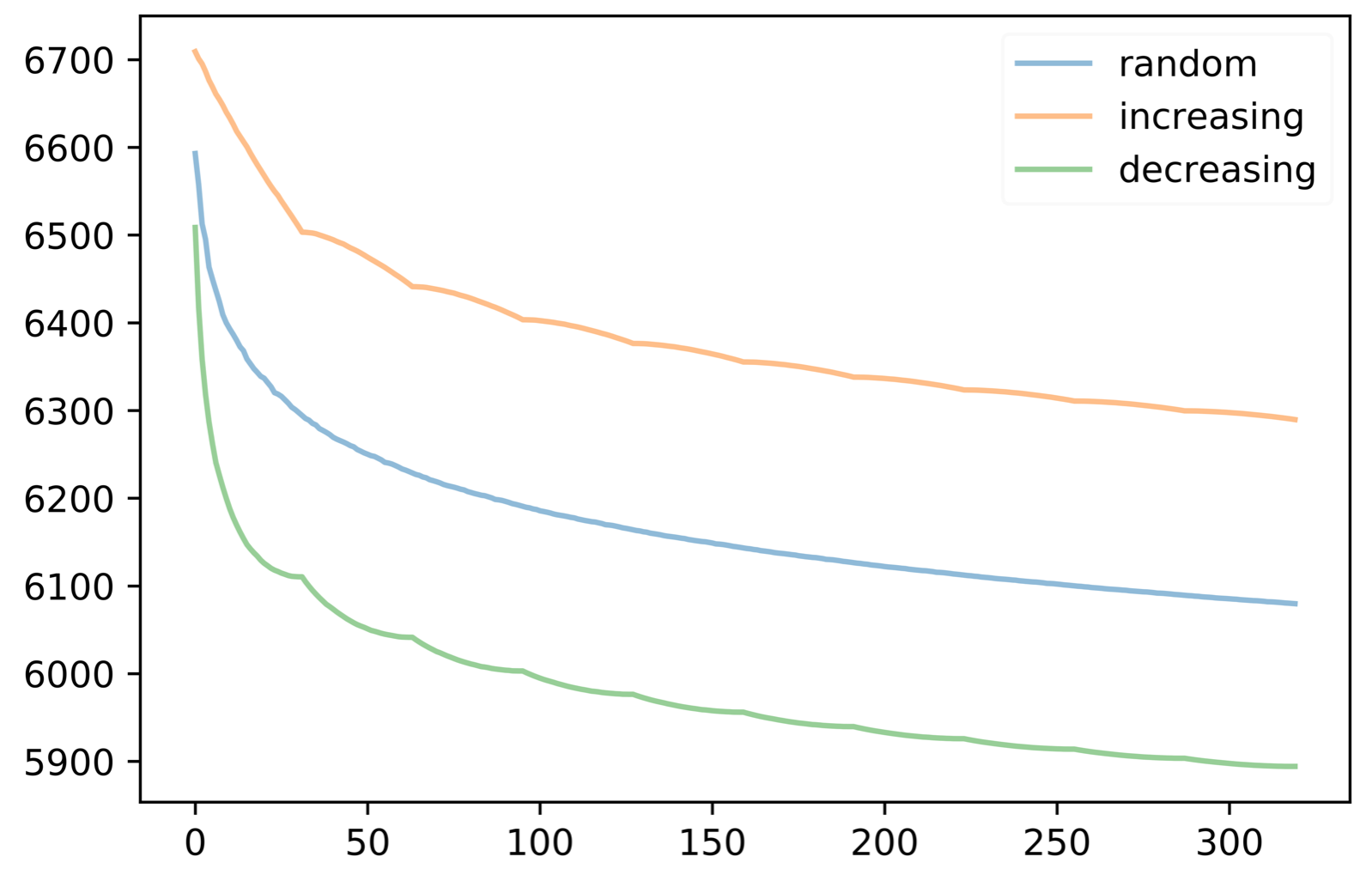
From the graph we could observe that for constant step size the loss value at the beginning and end of an epoch is approximately the same for the three orderings, which supports that convergence rate is same for all orderings when step size is constant. From the graph for decreasing step size per epoch, we could clearly observe a difference between the loss of the three orderings, which further validate our theoretical results.

To further explore the relationship between distance from the optimal and convergence for the different orderings, we conducted two different experiments.

First, we applied a different loss function: $F=\sum_{i=1}^{m}\mathbbm{1}_{x<0}||x-x^{*}||^{4}_{4}+(1-\mathbbm{1}_{x<0})||x-x^{*}||^{2}_{2}$ , where $\mathbbm{1}_{x<0}$ is the indicator function.

With the case when the initial value is [-9,-9], the result for decreasing step size per iteration is shown below in figure 9(a), where we can observe random ordering actually achieves a better result than decreasing gradient. This is because the initial value is too far from the optimal.

4.2 Iris Data Set

We also test the algorithm on the Iris data set which contain 150 vectors with 4 features (sepal length, sepal width, petal length, and petal width; denote as $x$ ) and 1 target (species; denote as y). Here we apply a simple linear regression model. The initial step size for this case is $6\cdot 10^{-4}$ . (To avoid overflow due to high power, we further multiply $10^{-10}$ in front of the gradients.) The loss function in this case is $F=\sum_{i=1}^{m}||(w^{T}x+b)-y||^{4}_{4}+||(w^{T}x+b)-y||^{2}_{2}$ .

Figure 2 plot loss vs iteration for constant step size, decreasing step size per iteration, and decreasing step size per epoch correspondingly.

Similar to the result from Synthetic data, for constant step size, the loss value is approximately the same for all orderings after an epoch; for decreasing step size, ordering by decreasing initial gradients results in the smallest loss value. These results further enhances our theoretical conclusion.

4.3 Boston Housing Data

We further test the algorithm on the Boston Housing data set which contain 560 vectors with 13 features (denote as $x$ ) and 1 target (price; denote as $y$ ). Here we also apply a simple linear regression model. The initial step size for this case is $6\cdot 10^{-4}$ . (To avoid overflow due to high power, we further multiply $10^{-10}$ in front of the gradients.) Similarly, $F=\sum_{i=1}^{m}||(w^{T}x+b)-y||^{4}_{4}+||(w^{T}x+b)-y||^{2}_{2}$ .

The following graph plot loss vs iteration for constant step size, decreasing step size per iteration, and decreasing step size per epoch correspondingly. The same relation persists and can be clearly observed.

4.4 Comparison with Data Selection Algorithm

In this section, we apply the proposed permutation combined with data selection with batches. For the algorithm, each batch is of size $s$ , and within each batch only $q$ data points with largest gradient is iterated. For all the algorithms, we first run random shuffling using the full data (as above) till the iterate is close enough to the optimal and then switch to the permutations being compared.

We apply the algorithm to the same three data sets above. Within each data set, we set $S$ as 0.3, 0.6, 0.8 of the original data size and $q$ as 0.18, 0.5, 0.8 of $S$ , with full results in Appendix 6.4.

For these algorithms, we order the $q$ iterates within each batch both randomly and by decreasing gradient norm. From the figures, we could observe that for this algorithm, ordering by decreasing gradient norm for the $q$ iterates results in smaller loss in synthetic and real data sets. Comparing with the none data-selection algorithms, data-selection algorithms with decreasing gradient ordering results in the best result.

4.5 Extending to Mini-Batches on Neural Networks

Non-convex functions can be split into finite small bounded segments such that each segment is convex. Intuitively, performing our proposed algorithm on these convex segments, we can at least reach a local minimal for the lost functions. Hence in the following experiments, we test our algorithms on larger data sets with both simple and more complex neural networks. (Full results in Appendix 6.5 and 6.6)

4.5.1 MNIST and Fashion MNIST Data set

We test our algorithm on the MNIST data set with two different neural network models: 2 layer and 7 layer. Both models are applied to each data set. The MNIST data set consists of images of handwritten digits, with 60,000 training images and 10,000 testing images. For the experiments, we iterate over 50 percent of samples within each mini-batch ( $q=0.5$ ), with batch sizes of 128 and 256 correspondingly. From the results, we could identify that in both training and testing, the mini-batch algorithm with less data and decreasing gradient ordering results in the highest accuracy. This supports that our gradient ordering can be combined with mini-batch on more complex models like neural networks to further improve convergence and decrease training time. (Full graphs can be found in Appendix 6.5).

To further investigate the performance of our algorithm on neural networks, we apply it to the Fashion MNIST Dataset, containing fashion images of clothing, with 60,000 training images and 10,000 testing images. Similarly, we perform the training with $q=0.5$ , and utilize the 2-layer and 7-layer networks as above. The mini-batch algorithms still outperform the algorithm training on full data on both models. In particular, the mini-batch algorithm with decreasing sorting results in the best performance. This result justifies that for adequate models, our ordering can be combined with mini-batch to further improve convergence (Full graphs can be found in Appendix 6.5).

4.5.2 CIFAR-10 and CIFAR-100 Data set

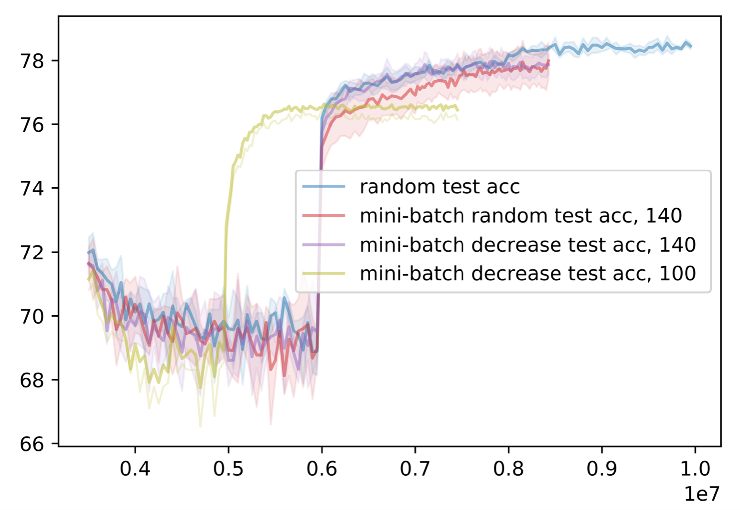
Approaching more complex data sets and networks, we validate our ordering and algorithm on CIFAR-10 and CIFAR-100 data sets with ResNet20 and ResNet18, respectively. The baseline result we are comparing with is training the network 200 epochs that achieves test accuracy about 92% for CIFAR-10 and about 79% for CIFAR-100. Due the complexity of the model, instead of sorting by decreasing gradient, we respectively sort by norm of logits, the performance of the model on the sample. Also, instead of calculating the permutation within each mini-batch, we calculate the total ordering at the beginning of the epoch to reduce calculation run-time. As a result, samples that are predicted worst (least learned) will be be first iterated in the epoch.

The highest test accuracy for mini-batch algorithms ( $q=0.5$ , using 50% of data from each mini-batch) is starting the corresponding ordering (random or increasing accuracy) at epoch 140. Comparing with training on full data, the mini-batch algorithm with less data and increasing accuracy ordering reaches the lowest training error with fewer amount of iterations. Though there is a slight difference in test accuracy, the difference is not too significant. (Full graphs can be found in Appendix 6.6).

	Train Loss	Train Acc	Test Loss	Test Acc
CIFAR-10 full random	0.019	99.72%	0.247	92.56 %
full ordered	0.014	99.81%	0.261	92.09 %
mini random	0.017	99.70%	0.253	92.72 %
mini ordered	0.010	99.94%	0.243	92.31 %
CIFAR-100 full random	0.017	99.93%	0.90	78.86 %
full ordered	0.013	99.98%	0.89	78.80 %
mini random	0.017	99.94%	0.91	78.71 %
mini ordered	0.010	99.99%	0.92	78.46 %

In addition, if we adjust the mini-batch ordering to begin at smaller epochs (epoch 80 for CIFAR-10 and epoch 100 for CIFAR-100), we can arrive at approximately similar low training error and high testing accuracy with significantly fewer epochs. Though with this approach the test accuracy is not the highest, the difference is negligible compared to the amount of time and calculation saved in training, at least $10^{6}$ iterations. (Full graphs can be found in Appendix 6.6).

5 Conclusion

In this paper, we explored the optimal ordering for shuffling algorithms which seek to improve the convergence of random shuffling: For decreasing step size per iteration, ordering by decreasing gradient at the beginning of the epoch results in a faster convergence rate; for constant step size, all orderings results in the same convergence rate. From experimental results we indeed verified the orderings and confirmed that the initial point should be sufficiently close to the optimal. Through comparison of different step size conditions we could observe for decreasing step size per epoch, the behavior varies for different data sets which suggests further analysis in the future. We also extended our results to mini-batch algorithms and non-convex settings with neural networks. Through empirical result, our ordering can be extended to these more complex settings. Further work is needed to theoretically explain the phenomenon.

References

[1] Pankaj K Agarwal, Sariel Har-Peled and Kasturi R Varadarajan “Approximating extent measures of points” In Journal of the ACM (JACM) 51.4 ACM New York, NY, USA, 2004, pp. 606–635
[2] Kwangjun Ahn, Chulhee Yun and Suvrit Sra “SGD with shuffling: optimal rates without component convexity and large epoch requirements” In Advances in Neural Information Processing Systems 33, 2020, pp. 17526–17535
[3] Guillaume Alain et al. “Variance Reduction in SGD by Distributed Importance Sampling”, 2015 eprint: arXiv:1511.06481
[4] Ellen Allen, Richard Helgason, Jeffery Kennington and Bala Shetty “A generalization of Polyak’s convergence result for subgradient optimization” In Mathematical Programming 37.3 Springer, 1987, pp. 309–317
[5] Zeyuan Allen-Zhu “Katyusha: The first direct acceleration of stochastic gradient methods” In The Journal of Machine Learning Research 18.1 JMLR. org, 2017, pp. 8194–8244
[6] Zeyuan Allen-Zhu, Yang Yuan and Karthik Sridharan “Exploiting the structure: Stochastic gradient methods using raw clusters” In Advances in Neural Information Processing Systems 29, 2016
[7] Hilal Asi and John C Duchi “The importance of better models in stochastic optimization” In Proceedings of the National Academy of Sciences 116.46 National Acad Sciences, 2019, pp. 22924–22930
[8] Jimmy Lei Ba, Jamie Ryan Kiros and Geoffrey E Hinton “Layer normalization” In arXiv preprint arXiv:1607.06450, 2016
[9] Francis Bach “Adaptivity of averaged stochastic gradient descent to local strong convexity for logistic regression” In The Journal of Machine Learning Research 15.1 JMLR. org, 2014, pp. 595–627
[10] Mokhtar S Bazaraa and Hanif D Sherali “On the choice of step size in subgradient optimization” In European Journal of Operational Research 7.4 Elsevier, 1981, pp. 380–388
[11] Dimitri Bertsekas “Convex optimization algorithms” Athena Scientific, 2015
[12] Dimitri P Bertsekas “Incremental least squares methods and the extended Kalman filter” In SIAM Journal on Optimization 6.3 SIAM, 1996, pp. 807–822
[13] Dimitri P Bertsekas “A hybrid incremental gradient method for least squares” In SIAM Journal on Optimization 7, 1997, pp. 913–926
[14] Dimitri P Bertsekas “Nonlinear programming” In Journal of the Operational Research Society 48.3 Taylor & Francis, 1997, pp. 334–334
[15] Dimitri P Bertsekas “Incremental gradient, subgradient, and proximal methods for convex optimization: A survey” In Optimization for Machine Learning 2010.1-38, 2011, pp. 3
[16] Dimitri P Bertsekas and John N Tsitsiklis “Neuro-dynamic programming: an overview” In Proceedings of 1995 34th IEEE conference on decision and control 1, 1995, pp. 560–564 IEEE
[17] Dimitri P Bertsekas and John N Tsitsiklis “Gradient convergence in gradient methods with errors” In SIAM Journal on Optimization 10.3 SIAM, 2000, pp. 627–642
[18] Léon Bottou and Yann Le Cun “On-line learning for very large data sets” In Applied stochastic models in business and industry 21.2 Wiley Online Library, 2005, pp. 137–151
[19] Stephen Boyd et al. “Distributed optimization and statistical learning via the alternating direction method of multipliers” In Foundations and Trends® in Machine learning 3.1 Now Publishers, Inc., 2011, pp. 1–122
[20] Ulf Brannlund “On relaxation methods for nonsmooth convex optimization.”, 1995
[21] Trevor Campbell and Tamara Broderick “Bayesian coreset construction via greedy iterative geodesic ascent” In International Conference on Machine Learning, 2018, pp. 698–706 PMLR
[22] Kai Lai Chung “On a stochastic approximation method” In The Annals of Mathematical Statistics JSTOR, 1954, pp. 463–483
[23] Michael B Cohen, Cameron Musco and Christopher Musco “Input sparsity time low-rank approximation via ridge leverage score sampling” In Proceedings of the Twenty-Eighth Annual ACM-SIAM Symposium on Discrete Algorithms, 2017, pp. 1758–1777 SIAM
[24] Rafael Correa and Claude Lemaréchal “Convergence of some algorithms for convex minimization” In Mathematical Programming 62.1 Springer, 1993, pp. 261–275
[25] Aaron Defazio, Francis Bach and Simon Lacoste-Julien “SAGA: A fast incremental gradient method with support for non-strongly convex composite objectives” In Advances in neural information processing systems 27, 2014
[26] Aaron Defazio and Léon Bottou “On the ineffectiveness of variance reduced optimization for deep learning” In Advances in Neural Information Processing Systems 32, 2019
[27] VF Dem’yanov and LV Vasil’ev “Nondifferentiable Optimization, Optimization Software” In Inc. Publications Division, New York, 1985
[28] John Duchi, Elad Hazan and Yoram Singer “Adaptive subgradient methods for online learning and stochastic optimization.” In Journal of machine learning research 12.7, 2011
[29] Yu M Ermol’ev “Methods of solution of nonlinear extremal problems” In Cybernetics 2.4 Springer, 1966, pp. 1–14
[30] Yu Ermoliev “Stochastic programming methods” Nauka, 1976
[31] Yu M Ermoliev “On the stochastic quasi-gradient method and stochastic quasi-Feyer sequences” In Kibernetika 2, 1969, pp. 72–83
[32] Yu M Ermoliev and RJ-B Wets “Numerical techniques for stochastic optimization” Springer-Verlag, 1988
[33] Yuri Ermoliev “Stochastic quasigradient methods and their application to system optimization” In Stochastics: An International Journal of Probability and Stochastic Processes 9.1-2 Taylor & Francis, 1983, pp. 1–36
[34] Roy Frostig, Rong Ge, Sham Kakade and Aaron Sidford “Un-regularizing: approximate proximal point and faster stochastic algorithms for empirical risk minimization” In International Conference on Machine Learning, 2015, pp. 2540–2548 PMLR
[35] Alexei A Gaivoronski “Convergence properties of backpropagation for neural nets via theory of stochastic gradient methods. Part 1” In Optimization methods and Software 4.2 Taylor & Francis, 1994, pp. 117–134
[36] Xavier Glorot and Yoshua Bengio “Understanding the difficulty of training deep feedforward neural networks” In Proceedings of the thirteenth international conference on artificial intelligence and statistics, 2010, pp. 249–256 JMLR WorkshopConference Proceedings
[37] Jean-Louis Goffin “The relaxation method for solving systems of linear inequalities” In Mathematics of Operations Research 5.3 INFORMS, 1980, pp. 388–414
[38] Jean-Louis Goffin and Krzysztof C Kiwiel “Convergence of a simple subgradient level method” In Mathematical Programming 85.1 Springer-Verlag, 1999, pp. 207–211
[39] Luigi Grippo “A class of unconstrained minimization methods for neural network training” In Optimization Methods and Software 4.2 Taylor & Francis, 1994, pp. 135–150
[40] M Gurbuzbalaban, Asu Ozdaglar and Pablo A Parrilo “Convergence rate of incremental gradient and incremental newton methods” In SIAM Journal on Optimization 29.4 SIAM, 2019, pp. 2542–2565
[41] Mert Gurbuzbalaban, Asuman Ozdaglar and Pablo A Parrilo “On the convergence rate of incremental aggregated gradient algorithms” In SIAM Journal on Optimization 27.2 SIAM, 2017, pp. 1035–1048
[42] Mert Gürbüzbalaban, Asuman Ozdaglar and Pablo Parrilo “A globally convergent incremental Newton method” In Mathematical Programming 151.1 Springer, 2015, pp. 283–313
[43] Mert Gürbüzbalaban, Asuman Ozdaglar and Pablo Parrilo “Why Random Reshuffling Beats Stochastic Gradient Descent” In arXiv preprint arXiv:1510.08560, 2015
[44] Jeff Haochen and Suvrit Sra “Random shuffling beats sgd after finite epochs” In International Conference on Machine Learning, 2019, pp. 2624–2633 PMLR
[45] Sariel Har-Peled and Soham Mazumdar “On coresets for k-means and k-median clustering” In Proceedings of the thirty-sixth annual ACM symposium on Theory of computing, 2004, pp. 291–300
[46] Elad Hazan, Amit Agarwal and Satyen Kale “Logarithmic regret algorithms for online convex optimization” In Machine Learning 69.2 Springer, 2007, pp. 169–192
[47] Jean-Baptiste Hiriart-Urruty and Claude Lemaréchal “Convex analysis and minimization algorithms I: Fundamentals” Springer science & business media, 2013
[48] Thomas Hofmann, Aurelien Lucchi, Simon Lacoste-Julien and Brian McWilliams “Variance reduced stochastic gradient descent with neighbors” In Advances in Neural Information Processing Systems 28, 2015
[49] Sergey Ioffe and Christian Szegedy “Batch Normalization: Accelerating Deep Network Training by Reducing Internal Covariate Shift” In CoRR abs/1502.03167, 2015
[50] Rie Johnson and Tong Zhang “Accelerating stochastic gradient descent using predictive variance reduction” In Advances in neural information processing systems 26, 2013
[51] Christos A Kaskavelis and Michael C Caramanis “Efficient Lagrangian relaxation algorithms for industry size job-shop scheduling problems” In IIE transactions 30.11 Springer, 1998, pp. 1085–1097
[52] Angelos Katharopoulos and François Fleuret “Not all samples are created equal: Deep learning with importance sampling” In International conference on machine learning, 2018, pp. 2525–2534 PMLR
[53] L Kaufman, PJ Rousseeuw and Y Dodge “Clustering by means of medoids in statistical data analysis based on the” In L1 Norm,~ orth-Holland, Amsterdam, 1987
[54] Kenji Kawaguchi and Haihao Lu “Ordered SGD: A new stochastic optimization framework for empirical risk minimization” In International Conference on Artificial Intelligence and Statistics, 2020, pp. 669–679 PMLR
[55] Sehun Kim, Hyunsil Ahn and Seong-Cheol Cho “Variable target value subgradient method” In Mathematical Programming 49.1 Springer, 1990, pp. 359–369
[56] Sehun Kim and Bong-sik Um “An improved subgradient method for constrained nondifferentiable optimization” In Operations Research Letters 14.1 Elsevier, 1993, pp. 61–64
[57] Diederik P Kingma and Jimmy Ba “Adam: A method for stochastic optimization” In arXiv preprint arXiv:1412.6980, 2014
[58] Krzysztof C Kiwiel “The efficiency of subgradient projection methods for convex optimization, part I: General level methods” In SIAM Journal on Control and Optimization 34.2 SIAM, 1996, pp. 660–676
[59] Krzysztof C Kiwiel “The efficiency of subgradient projection methods for convex optimization, part II: Implementations and extensions” In SIAM Journal on Control and Optimization 34.2 SIAM, 1996, pp. 677–697
[60] Krzysztof C Kiwiel, Torbjörn Larsson and Per Olov Lindberg “The efficiency of ballstep subgradient level methods for convex optimization” In Mathematics of Operations Research 24.1 INFORMS, 1999, pp. 237–254
[61] Teuvo Kohonen “An adaptive associative memory principle” In IEEE Transactions on Computers 100.4 IEEE, 1974, pp. 444–445
[62] Anatolii Nikolaevich Kulikov and Valeriy Raufovich Fazylov “Convex optimization with prescribed accuracy” In USSR computational mathematics and mathematical physics 30.3 Elsevier, 1990, pp. 16–22
[63] Mu Li, Gary L Miller and Richard Peng “Iterative row sampling” In 2013 IEEE 54th Annual Symposium on Foundations of Computer Science, 2013, pp. 127–136 IEEE
[64] Hongzhou Lin, Julien Mairal and Zaid Harchaoui “A universal catalyst for first-order optimization” In Advances in neural information processing systems 28, 2015
[65] Hui Lin, Jeff Bilmes and Shasha Xie “Graph-based submodular selection for extractive summarization” In 2009 IEEE Workshop on Automatic Speech Recognition & Understanding, 2009, pp. 381–386 IEEE
[66] Hui Lin and Jeff A Bilmes “Learning mixtures of submodular shells with application to document summarization” In arXiv preprint arXiv:1210.4871, 2012
[67] Yucheng Lu, Si Yi Meng and Christopher De Sa “A General Analysis of Example-selection for Stochastic Gradient Descent” In conference paper at ICLR 2022, 2022
[68] Mario Lucic, Matthew Faulkner, Andreas Krause and Dan Feldman “Training gaussian mixture models at scale via coresets” In The Journal of Machine Learning Research 18.1 JMLR. org, 2017, pp. 5885–5909
[69] Zhi-Quan Luo “On the convergence of the LMS algorithm with adaptive learning rate for linear feedforward networks” In Neural Computation 3.2 MIT Press One Rogers Street, Cambridge, MA 02142-1209, USA journals-info …, 1991, pp. 226–245
[70] Olvi L Mangasarian and Mikhail V Solodov “Backpropagation convergence via deterministic nonmonotone perturbed minimization” In Advances in Neural Information Processing Systems 6, 1993
[71] Michel Minoux “Accelerated greedy algorithms for maximizing submodular set functions” In Optimization techniques Springer, 1978, pp. 234–243
[72] Michel Minoux “Mathematical programming: theory and algorithms” John Wiley & Sons, 1986
[73] Baharan Mirzasoleiman et al. “Lazier than lazy greedy” In Proceedings of the AAAI Conference on Artificial Intelligence 29.1, 2015
[74] Baharan Mirzasoleiman, Jeff Bilmes and Jure Leskovec “Coresets for data-efficient training of machine learning models” In International Conference on Machine Learning, 2020, pp. 6950–6960 PMLR
[75] Baharan Mirzasoleiman, Amin Karbasi, Ashwinkumar Badanidiyuru and Andreas Krause “Distributed submodular cover: Succinctly summarizing massive data” In Advances in Neural Information Processing Systems 28, 2015
[76] Baharan Mirzasoleiman, Morteza Zadimoghaddam and Amin Karbasi “Fast distributed submodular cover: Public-private data summarization” In Advances in Neural Information Processing Systems 29, 2016
[77] Konstantin Mishchenko, Ahmed Khaled Ragab Bayoumi and Peter Richtarik “Random Reshuffling: Simple Analysis with Vast Improvements” In Advances in Neural Information Processing Systems 33: Annual Conference on Neural Information Processing Systems 2020, NeurIPS 2020, December 6-12, 2020, virtual, 2020 URL: https://proceedings.neurips.cc/paper/2020/hash/c8cc6e90ccbff44c9cee23611711cdc4-Abstract.html
[78] Amirkeivan Mohtashami, Sebastian U. Stich and Martin Jaggi “Characterizing & Finding Good Data Orderings for Fast Convergence of Sequential Gradient Methods” In ArXiv abs/2202.01838, 2022
[79] Hiroyuki Moriyama, Nobuo Yamashita and Masao Fukushima “The incremental Gauss-Newton algorithm with adaptive stepsize rule” In Computational Optimization and Applications 26.2 Springer, 2003, pp. 107–141
[80] Eric Moulines and Francis Bach “Non-asymptotic analysis of stochastic approximation algorithms for machine learning” In Advances in neural information processing systems 24, 2011
[81] Cameron Musco and Christopher Musco “Recursive sampling for the nystrom method” In Advances in Neural Information Processing Systems 30, 2017
[82] Angelia Nedic and Dimitri P Bertsekas “Incremental subgradient methods for nondifferentiable optimization” In SIAM Journal on Optimization 12.1 SIAM, 2001, pp. 109–138
[83] Angelia Nedic and Asuman Ozdaglar “On the rate of convergence of distributed subgradient methods for multi-agent optimization” In 2007 46th IEEE Conference on Decision and Control, 2007, pp. 4711–4716 IEEE
[84] Angelia Nedic and Asuman Ozdaglar “Distributed subgradient methods for multi-agent optimization” In IEEE Transactions on Automatic Control 54.1 IEEE, 2009, pp. 48–61
[85] Angelia Nedić and Dimitri Bertsekas “Convergence rate of incremental subgradient algorithms” In Stochastic optimization: algorithms and applications Springer, 2001, pp. 223–264
[86] Deanna Needell, Rachel Ward and Nati Srebro “Stochastic gradient descent, weighted sampling, and the randomized Kaczmarz algorithm” In Advances in neural information processing systems 27, 2014
[87] George L Nemhauser, Laurence A Wolsey and Marshall L Fisher “An analysis of approximations for maximizing submodular set functions—I” In Mathematical programming 14.1 Springer, 1978, pp. 265–294
[88] Arkadi Nemirovski, Anatoli Juditsky, Guanghui Lan and Alexander Shapiro “Robust stochastic approximation approach to stochastic programming” In SIAM Journal on optimization 19.4 SIAM, 2009, pp. 1574–1609
[89] Yurii Nesterov “Introductory lectures on convex optimization: a basic course”, 2004
[90] Lam M. Nguyen et al. “A Unified Convergence Analysis for Shuffling-Type Gradient Methods” In Journal of Machine Learning Research, 2021, pp. 1–44
[91] Elijah Polak “On the mathematical foundations of nondifferentiable optimization in engineering design” In SIAM review 29.1 SIAM, 1987, pp. 21–89
[92] Boris T Polyak “Introduction to optimization. optimization software” In Inc., Publications Division, New York 1, 1987, pp. 32
[93] Boris Teodorovich Polyak “A general method for solving extremal problems” In Doklady Akademii Nauk 174.1, 1967, pp. 33–36 Russian Academy of Sciences
[94] Boris Teodorovich Polyak “Minimization of unsmooth functionals” In USSR Computational Mathematics and Mathematical Physics 9.3 Elsevier, 1969, pp. 14–29
[95] Ning Qian “On the momentum term in gradient descent learning algorithms” In Neural networks 12.1 Elsevier, 1999, pp. 145–151
[96] Shashank Rajput, Anant Gupta and Dimitris Papailiopoulos “Closing the convergence gap of SGD without replacement” In ICML’20: Proceedings of the 37th International Conference on Machine Learning, 2020, pp. 7964–7973
[97] Shashank Rajput, Kangwook Lee and Dimitris Papailiopoulos “Permutation-Based SGD: Is Random Optimal?” In International Conference on Learning Representations, 2022 URL: https://openreview.net/forum?id=YiBa9HKTyXE
[98] Alexander Rakhlin, Ohad Shamir and Karthik Sridharan “Making gradient descent optimal for strongly convex stochastic optimization” In arXiv preprint arXiv:1109.5647, 2011
[99] S Sundhar Ram, A Nedic and VV Veeravalli “Stochastic incremental gradient descent for estimation in sensor networks” In 2007 conference record of the forty-first asilomar conference on signals, systems and computers, 2007, pp. 582–586 IEEE
[100] R Tyrrell Rockafellar “Convex Analysis” Citeseer, 1970
[101] Nicolas Roux, Mark Schmidt and Francis Bach “A stochastic gradient method with an exponential convergence _rate for finite training sets” In Advances in neural information processing systems 25, 2012
[102] Itay Safran and Ohad Shamir “How good is SGD with random shuffling?” In Conference on Learning Theory, 2020, pp. 3250–3284 PMLR
[103] Vatsal Shah, Xiaoxia Wu and Sujay Sanghavi “Choosing the Sample with Lowest Loss makes SGD Robust” In International Conference on Artificial Intelligence and Statistics, 2020
[104] Shai Shalev-Shwartz and Tong Zhang “Stochastic dual coordinate ascent methods for regularized loss minimization.” In Journal of Machine Learning Research 14.2, 2013
[105] Ohad Shamir “Without-Replacement Sampling for Stochastic Gradient Methods: Convergence Results and Application to Distributed Optimization”, 2016 eprint: arXiv:1603.00570
[106] NZ Shor, Krzysztof C Kiwiel and Andrzej Ruszcaynski “Minimization methods for non-differentiable functions” Springer-Verlag, 1985
[107] Jascha Sohl-Dickstein, Ben Poole and Surya Ganguli “Fast large-scale optimization by unifying stochastic gradient and quasi-Newton methods” In International Conference on Machine Learning, 2014, pp. 604–612 PMLR
[108] Mikhail V Solodov “Incremental gradient algorithms with stepsizes bounded away from zero” In Computational Optimization and Applications 11.1 Springer, 1998, pp. 23–35
[109] Mikhail V Solodov and SK Zavriev “Error stability properties of generalized gradient-type algorithms” In Journal of Optimization Theory and Applications 98.3 Springer, 1998, pp. 663–680
[110] Evan R Sparks et al. “MLI: An API for distributed machine learning” In 2013 IEEE 13th International Conference on Data Mining, 2013, pp. 1187–1192 IEEE
[111] Sebastian U. Stich, Anant Raj and Martin Jaggi “Safe Adaptive Importance Sampling”, 2017 eprint: arXiv:1711.02637
[112] Emma Strubell, Ananya Ganesh and Andrew McCallum “Energy and policy considerations for deep learning in NLP” In arXiv preprint arXiv:1906.02243, 2019
[113] Paul Tseng “An incremental gradient (-projection) method with momentum term and adaptive stepsize rule” In SIAM Journal on Optimization 8.2 SIAM, 1998, pp. 506–531
[114] Kai Wei, Rishabh Iyer and Jeff Bilmes “Submodularity in data subset selection and active learning” In International Conference on Machine Learning, 2015, pp. 1954–1963 PMLR
[115] Laurence A Wolsey “An analysis of the greedy algorithm for the submodular set covering problem” In Combinatorica 2.4 Springer, 1982, pp. 385–393
[116] Lin Xiao and Tong Zhang “A proximal stochastic gradient method with progressive variance reduction” In SIAM Journal on Optimization 24.4 SIAM, 2014, pp. 2057–2075
[117] Chulhee Yun, Suvrit Sra and Ali Jadbabaie “Open Problem: Can Single-Shuffle SGD be Better than Reshuffling SGD and GD?” In Conference on Learning Theory, 2021, pp. 4653–4658 PMLR
[118] Matthew D Zeiler “Adadelta: an adaptive learning rate method” In arXiv preprint arXiv:1212.5701, 2012
[119] Xing Zhao, Peter B Luh and Jihua Wang “Surrogate gradient algorithm for Lagrangian relaxation” In Journal of optimization Theory and Applications 100.3 Springer, 1999, pp. 699–712
[120] Luo Zhi-Quan and Tseng Paul “Analysis of an approximate gradient projection method with applications to the backpropagation algorithm” In Optimization Methods and Software 4.2 Taylor & Francis, 1994, pp. 85–101

6 Appendix

6.1 Proof of Lemma 1

Proof.

By property of convex functions, we have for $\forall x$

\begin{array}[]{l@{}l}f_{i}(x^{*})&\geq f_{i}(x)+\nabla f_{i}(x)^{T}(x^{*}-x)\\ f_{i}(x^{*})-f_{i}(x)&\geq\nabla f_{i}(x)^{T}(x^{*}-x)\\ f_{i}(x)-f_{i}(x^{*})&\leq\nabla f_{i}(x)^{T}(x-x^{*})\\ f_{i}(x)-f_{i}(x^{*})&\leq||\nabla f_{i}(x)^{T}(x-x^{*})||\leq||\nabla f_{i}(x)^{T}||||(x-x^{*})||\end{array}

(10)

Here we used the property that $f_{i}(x)\geq f_{i}(x^{*})$ for all i, and $||AB||\leq||A||||B||$ .
Since the $||x-x^{*}||$ is constant at each iteration, then the larger the $||\nabla f_{i}(x)^{T}||$ , the larger the upper bound for $f_{i}(x)-f_{i}(x^{*})$ .
∎

Proof of Theorems 1 and 2

Proof.

Following the proof from Convergence Rate of Incremental Subgradient Algorithms([85]), we have the following:

\begin{array}[]{l@{}l}||x_{i,k}-x^{*}||^{2}&=||P_{x}[x_{i-1,k}-\alpha_{i,k}g_{i,k}]-x^{*}||^{2}\\ &{}\leq||x_{i-1,k}-\alpha_{i,k}g_{i,k}-x^{*}||^{2}\\ &{}\leq||x_{i-1,k}-x^{*}||^{2}-2\alpha_{i,k}g_{i,k}\cdot(x_{i-1,k}-x^{*})+\alpha_{i,k}^{2}g_{i,k}^{2}\\ &{}\leq||x_{i-1,k}-x^{*}||^{2}-2\alpha_{i,k}g_{i,k}\cdot(x_{i-1,k}-x^{*})+\alpha_{k}^{2}C_{i}^{2}\\ &{}\leq||x_{i-1,k}-x^{*}||^{2}-2\alpha_{i,k}\cdot(f_{i}(x_{i-1,k})-f_{i}(x^{*}))+\alpha_{k}^{2}C_{i}^{2}\\ \end{array}

(11)

If we add the above relation for all points within a epoch we get:

||x_{k+1}-x^{*}||^{2}\leq||x_{k}-x^{*}||^{2}-2\sum_{i=1}^{n}[\alpha_{i,k}\cdot(f_{i}(x_{i-1,k})-f_{i}(x^{*}))]+\alpha_{k}^{2}\sum_{i=1}^{n}C^{2}

(12)

Since $\alpha_{i,k}$ is decreasing, to minimize the upper bound for $||x_{k+1}-x^{*}||^{2}$ , we have to maximize $f_{i}(x_{i-1,k})-f_{i}(x^{*})$ for each iteration and have the larger values be in the beginning with the larger $\alpha_{i,k}$ . Hence it’s reasonable to have the $f_{i}(x_{i-1,k})-f_{i}(x^{*})$ with larger upper bounds in the beginning.

To maximize $\sum_{i=1}^{n}[\alpha_{i,k}\cdot(f_{i}(x_{i-1,k})-f_{i}(x^{*}))]$ , we will order the $f_{i}$ such that the $f_{i}$ ’s with larger values of $f_{i}(x_{i-1})-f_{i}(x^{*})$ are iterated first.
Let $|M_{1}|>|M_{2}|>|M_{3}|>...>|M_{n}|$ be the magnitude of the sub-gradients in the beginning of the epoch, and denote $f_{1},f_{2},f_{3},...,f_{n}$ the corresponding function for those sub-gradients.

For the first iteration, it’s obvious that choosing $f_{1}$ with the largest $|M_{i}|$ would maximize upper bound for $f_{i}(x_{0})-f_{i}(x^{*})$ .
For the following iterations, instead of directly finding the maximum value for $f_{i}(x)-f_{i}(x^{*})$ , we compare the lower bound $f_{i}(x)-f_{i}(x^{*})$ . Through ordering by that value, we can bound the minimum value of $f_{i}(x_{i-1,k})-f_{i}(x^{*})$ .

For the second iteration:
we first compare $f_{2}$ and $f_{3}$ . Note $x_{1,k}=x_{0,k}-\alpha_{1,k}M_{1}$ .

\begin{array}[]{l@{}l}f_{2}(x_{0,k}-\alpha_{1,k}M_{1})-f_{2}(x^{*})&\geq f_{2}(x_{0,k})-\nabla f_{2}(x_{0,k})^{T}(\alpha_{1,k}M_{1})+\frac{m_{2}}{2}||\alpha_{1,k}M_{1}||^{2}-f_{2}(x^{*})\\ &{}\geq[f_{2}(x_{0,k})-f_{2}(x^{*})]-\alpha_{1,k}||M_{1}||^{2}+\frac{m_{2}\alpha_{1,k}^{2}}{2}||M_{1}||^{2}\\ f_{3}(x_{0,k}-\alpha_{1,k}M_{1})-f_{3}(x^{*})&\geq f_{3}(x_{0,k})-\nabla f_{3}(x_{0,k})^{T}(\alpha_{1,k}M_{1})+\frac{m_{3}}{2}||\alpha_{1,k}M_{1}||^{2}-f_{3}(x^{*})\\ &{}\geq[f_{3}(x_{0,k})-f_{3}(x^{*})]-\alpha_{1,k}||M_{1}||^{2}+\frac{m_{3}\alpha_{1,k}^{2}}{2}||M_{1}||^{2}\\ \end{array}

(13)

Since $\alpha$ is small, $\alpha^{2}$ is insignificant compared with the rest of the terms, and can be treated as a error.
Since $||M_{2}||\geq||M_{3}||$ ,
$upperbound(f_{2}(x_{0,k})-f_{2}(x^{*}))\geq upperbound(f_{3}(x_{0,k})-f_{3}(x^{*}))$
Hence, at the second iteration, we know $f_{2}(x_{1,k})-f_{2}(x^{*})$ more likely has a relative larger value for the lower bound than $f_{3}(x_{1,k})-f_{3}(x^{*})$ . Following the same logic, we can show relatively $lowerbound(f_{2}(x_{1,k})-f_{2}(x^{*}))$ more likely have a larger value than $lowerbound(f_{k}(x_{1,k})-f_{k}(x^{*}))$ for $k>2$ . Thus it is optimal to have $f_{2}$ at the second iteration.

Assume the above relation hold for iterations 1, 2, …, N-1.
For the $N^{th}$ iteration:
$x_{N,k}=x_{0,k}-\sum_{i=1}^{N-1}\alpha_{i,k}M_{i}^{{}^{\prime}}$ ( $M_{i}^{{}^{\prime}}$ is the sub-gradient value in iteration i).

\begin{array}[]{l@{}}f_{N}(x_{0,k}-\sum_{i=1}^{N-1}\alpha_{i,k}M_{i}^{{}^{\prime}})-f_{N}(x^{*})\\ \geq f_{N}(x_{0,k})-\nabla f_{N}(x_{0,k})^{T}(\sum_{i=1}^{N-1}\alpha_{i,k}M_{i}^{{}^{\prime}})+\frac{m_{N}}{2}\sum_{i=1}^{N-1}||\alpha_{i,k}M_{i}^{{}^{\prime}}||^{2}-f_{N}(x^{*})\\ \geq[f_{N}(x_{0,k})-f_{N}(x^{*})]-\sum_{i=1}^{N-1}\alpha_{i,k}\max{(||M_{i}||,||M_{i}^{{}^{\prime}}||)}^{2}+\frac{m_{N}}{2}\sum_{i=1}^{N-1}||\alpha_{i,k}M_{i}^{{}^{\prime}}||^{2}\\ \\ f_{N+1}(x_{0,k}-\sum_{i=1}^{N-1}\alpha_{i,k}M_{i}^{{}^{\prime}})-f_{N+1}(x^{*})\\ \geq f_{N+1}(x_{0,k})-\nabla f_{N+1}(x_{0,k})^{T}(\sum_{i=1}^{N-1}\alpha_{i,k}M_{i}^{{}^{\prime}})+\frac{m_{N+1}}{2}\sum_{i=1}^{N-1}||\alpha_{i,k}M_{i}^{{}^{\prime}}||^{2}-f_{N+1}(x^{*})\\ \geq[f_{N+1}(x_{0,k})-f_{N+1}(x^{*})]-\sum_{i=1}^{N-1}\alpha_{i,k}\max{(||M_{i}||,||M_{i}^{{}^{\prime}}||)}^{2}+\frac{m_{N+1}}{2}\sum_{i=1}^{N-1}||\alpha_{i,k}M_{i}^{{}^{\prime}}||^{2}\\ \end{array}

(14)

Following the same argument as the second iteration we can see $lowerbound(f_{N}(x_{N-1,k})-f_{N}(x^{*}))$ has a larger value than $lowerbound(f_{N+1}(x_{N-1,k})-f_{N+1}(x^{*}))$ , and if we compare $f_{N}$ with $f_{k}$ where $k>N$ , we can get $lowerbound(f_{N}(x_{N-1,k})-f_{N}(x^{*}))$ has a larger amount than $lowerbound(f_{k}(x_{N-1,k})-f_{k}(x^{*}))$ .
Thus it is optimal to have $f_{N}$ at the $N^{th}$ iteration.

Thus by induction, through ordering the iteration by the sub-gradient value at the beginning of the epoch we maximize the lower bound of $f_{i}(x_{i-1,k})$ . This in turn help us derive a stricter upper bound for $||x_{k+1}-x^{*}||^{2}$ .
Plugging the above bound in formula (9), we get:

\begin{array}[]{l@{}l}||x_{k+1}-x^{*}||^{2}\\ \leq||x_{k}-x^{*}||^{2}-2\sum_{i=1}^{n}[\alpha_{i,k}\cdot(f_{i}(x_{i-1,k})-f_{i}(x^{*}))]+\alpha_{k}^{2}\sum_{i=1}^{n}C_{i}^{2}\\ \leq||x_{k}-x^{*}||^{2}-2\sum_{i=1}^{n}\alpha_{i,k}\left((f_{i}(x_{0,k})-f_{i}(x^{*}))-\sum_{j=1}^{i-1}\alpha_{j,k}\max{(||M_{j}||,||M_{j}^{{}^{\prime}}||)}^{2}+\frac{m_{i}}{2}\sum_{j=1}^{i-1}||\alpha_{j,k}M_{j}^{{}^{\prime}}||^{2}\right)\\ +\alpha_{k}^{2}\sum_{i=1}^{n}C_{i}^{2}\\ \leq||x_{k}-x^{*}||^{2}-2\sum_{i=1}^{n}\alpha_{i,k}(f_{i}(x_{k})-f_{i}(x^{*}))+\sum_{i=1}^{n}\left(\alpha_{i,k}\sum_{j=1}^{i-1}\max{(||M_{j}||,||M_{j}^{{}^{\prime}}||)}^{2}(2\alpha_{j,k}-m_{i}\alpha_{j,k}^{2})\right)\\ +\alpha_{k}^{2}\sum_{i=1}^{n}C_{i}^{2}\\ \leq||x_{k}-x^{*}||^{2}-2\sum_{i=1}^{n}\alpha_{i,k}(||M_{i}||||x_{k}-x^{*}||)+\alpha_{k}^{2}\left(2\sum_{i=1}^{n-1}[(n-i)C_{i}^{2}]+\sum_{i=1}^{n}C_{i}^{2}\right)\\ -\alpha_{k}^{2}\alpha_{k+1}\sum_{i=1}^{n-1}(n-i)m_{i}\cdot max{(||M_{i}||,||M_{i}^{{}^{\prime}}||)}^{2}+n\alpha_{k}\cdot\epsilon_{k}\\ \end{array}

(15)

where $\epsilon_{k}$ is the max error between $f_{i}(x_{k})-f_{i}(x^{*})$ and $||M_{i}||||x_{k}-x^{*}||$ in epoch k. We will assume that $\epsilon_{k}$ is small so that $m\alpha_{k}\cdot\epsilon_{k}$ is negligible.
For the case with decreasing step size per iteration:

\begin{array}[]{l@{}l}||x_{k+1}-x^{*}||^{2}\leq||x_{k}-x^{*}||^{2}-2||x_{k}-x^{*}||\sum_{i=1}^{n}\alpha_{i,k}||M_{i}||+\alpha_{k}^{2}\left(2\sum_{i=1}^{n-1}[(n-i)C_{i}^{2}]+\sum_{i=1}^{n}C_{i}^{2}\right)\\ -\alpha_{k}^{2}\alpha_{k+1}\sum_{i=1}^{n-1}(n-i)m_{i}\cdot max{(||M_{i}||,||M_{i}^{{}^{\prime}}||)}^{2}+n\alpha_{k}\cdot\epsilon_{k}\end{array}

(16)

In this case, since $\alpha_{i,k}$ decreases with each iteration, to minimize the upper bound we need to maximize $\sum_{i=1}^{n}\alpha_{i,k}||M_{i}||$ , which is attained when we order by decreasing order of the gradient at the beginning of the epoch. Also with the decreasing order, in expectation $\sum_{i=1}^{n}C_{i}^{2}$ is the smallest. The $\alpha_{k}^{2}$ and $\alpha_{k}^{2}\alpha_{k+1}$ are so small in magnitude compared to the prior terms that its value is negligible. Hence such ordering minimizes the upper bound, suggesting better convergence rate compared to other ordering.

For the case with constant step size, the expression can be simplified as:

\begin{array}[]{l@{}l}||x_{k+1}-x^{*}||^{2}\leq||x_{k}-x^{*}||^{2}-2\alpha||x_{k}-x^{*}||\sum_{i=1}^{n}||M_{i}||+\alpha^{2}\left(2\sum_{i=1}^{n-1}[(n-i)C_{i}^{2}]+\sum_{i=1}^{n}C_{i}^{2}\right)\\ -\alpha^{3}\sum_{i=1}^{n-1}(n-i)m_{i}\cdot max{(||M_{i}||,||M_{i}^{{}^{\prime}}||)}^{2}+n\alpha\cdot\epsilon_{k}\end{array}

(17)

In this case, $||x_{k}-x^{*}||$ and $\alpha$ are constant within an epoch. Though in expectation $\sum_{i=1}^{n}C_{i}^{2}$ is the smallest when we order by decreasing gradient order, the $\alpha^{2}$ and $\alpha^{3}$ are so small in magnitude compared to the prior terms that the different is negligible. Hence, no matter how we order the data points, the upper bound after an epoch is approximately the same, suggesting similar convergence rate.
∎

6.2 Proof of Theorems 3 and 4

Proof.

Following the same logic as the proof form Theorems 1 and 2, we result:

\begin{array}[]{l@{}l}||x_{k+1}-x^{*}||^{2}\\ \leq||x_{k}-x^{*}||^{2}-2\sum_{i=1}^{n}[\alpha_{i,k}\cdot(f_{i}(x_{i-1,k})-f_{i}(x^{*}))]+\alpha_{k}^{2}\sum_{i=1}^{n}C_{i}^{2}\\ \leq||x_{k}-x^{*}||^{2}-2\sum_{i=1}^{n}\alpha_{i,k}\left((f_{i}(x_{0,k})-f_{i}(x^{*}))-\sum_{j=1}^{i-1}\alpha_{j,k}\max{(||M_{j}||,||M_{j}^{{}^{\prime}}||)}^{2}\right)+\alpha_{k}^{2}\sum_{i=1}^{n}C_{i}^{2}\\ \leq||x_{k}-x^{*}||^{2}-2\sum_{i=1}^{n}\alpha_{i,k}(f_{i}(x_{k})-f_{i}(x^{*}))+\sum_{i=1}^{n}\left(2\alpha_{i,k}\sum_{j=1}^{i-1}\alpha_{j,k}\max{(||M_{j}||,||M_{j}^{{}^{\prime}}||)}^{2}\right)+\alpha_{k}^{2}\sum_{i=1}^{n}C_{i}^{2}\\ \leq||x_{k}-x^{*}||^{2}-2\sum_{i=1}^{n}\alpha_{i,k}(||M_{i}||||x_{k}-x^{*}||)+\alpha_{k}^{2}\left(2\sum_{i=1}^{n-1}[(n-i)C_{i}^{2}]+\sum_{i=1}^{n}C_{i}^{2}\right)+n\alpha_{k}\cdot\epsilon_{k}\\ \end{array}

(18)

For the case with decreasing step size per iteration:

\begin{array}[]{l@{}l}||x_{k+1}-x^{*}||^{2}\leq||x_{k}-x^{*}||^{2}-2||x_{k}-x^{*}||\sum_{i=1}^{n}\alpha_{i,k}||M_{i}||\\ \quad\quad\quad\quad+\alpha_{k}^{2}\left(2\sum_{i=1}^{n-1}[(n-i)C_{i}^{2}]+\sum_{i=1}^{n}C_{i}^{2}\right)+n\alpha_{k}\cdot\epsilon_{k}\end{array}

(19)

As in the strongly convex case, the best ordering that minimizes the upper bound is decreasing order of the gradients at the beginning of the epoch. For the case with constant step size, the expression can be simplified as:

\begin{array}[]{l@{}l}||x_{k+1}-x^{*}||^{2}\leq||x_{k}-x^{*}||^{2}-2\alpha||x_{k}-x^{*}||\sum_{i=1}^{n}||M_{i}||\\ \quad\quad\quad\quad+\alpha^{2}\left(2\sum_{i=1}^{n-1}[(n-i)C_{i}^{2}]+\sum_{i=1}^{n}C_{i}^{2}\right)+n\alpha\cdot\epsilon_{k}\end{array}

(20)

Following similar logic as the strongly convex case, all orderings for constant step size results in similar value of the upper bound. ∎

6.3 Distance from the Optimal

Here, we resumed to the original loss function for the synthesis data set and tried a new algorithm: first run random shuffling till the iterate is relative closer to the optimal and then switch to the proposed ordering. For the synthesis data, we ran 15 runs of random shuffling and then ran 10 runs of the assigned ordering. Observing the results shown in figure 9(b), ordering by decreasing initial gradient results in the smallest loss value, which further confirms our proposed ordering optimizes the convergence rate.

6.4 Full Results for Data Selection Algorithm Experiments

The results below are mini-batch algorithms applied to synthesis data set, Iris data set, and Boston Housing data set correspondingly.

For the $9x9$ ordered graphs, the rows correspond to the sizes of mini-match with respect to total data ( $S=0.3,0.6,0.8$ ), and the columns correspond to the training size within each mini-batch with respect to the batch size ( $q=0.18,0.5,0.8$ ).

6.5 Full Results for Experiments on Neural Networks with MNIST Data Sets

For the $2x2$ ordered graphs, the rows correspond to complexity of the model (2-layer or 7-layer), and the columns correspond to the mini-batch size ( $S=128,256$ ). For the experiments labeled mini-batch, $q=0.5$ .

The following results are from experiments for MNIST Data Set: