Order-sensitive Shapley Values for Evaluating Conceptual Soundness of NLP Models

Kaiji Lu ECE Department
Carnegie Mellon University
Pittsburgh, PA Anupam Datta ECE Department
Carnegie Mellon University
Pittsburgh, PA

Abstract

Previous works show that deep NLP models are not always conceptually sound: they do not always learn the correct linguistic concepts. Specifically, they can be insensitive to word order. In order to systematically evaluate models for their conceptual soundness with respect to word order, we introduce a new explanation method for sequential data: Order-sensitive Shapley Values (OSV). We conduct an extensive empirical evaluation to validate the method and surface how well various deep NLP models learn word order. Using synthetic data, we first show that OSV is more faithful in explaining model behavior than gradient-based methods. Second, applying to the HANS dataset, we discover that the BERT-based NLI model uses only the word occurrences without word orders. Although simple data augmentation improves accuracy on HANS, OSV shows that the augmented model does not fundamentally improve the model’s learning of order. Third, we discover that not all sentiment analysis models learn negation properly: some fail to capture the correct syntax of the negation construct. Finally, we show that pretrained language models such as BERT may rely on the absolute positions of subject words to learn long-range Subject-Verb Agreement. With each NLP task, we also demonstrate how OSV can be leveraged to generate adversarial examples.

Index Terms:

Machine Learning, Deep Learning, Natural Language Processing, Interpretability, Explainability

I Introduction

Recent works discover that NLP models are not sensitive to word orders in the same way as humans [1, 2, 3, 4, 5]: although randomly shuffled sentences are often incomprehensible to humans, they result in very small performance drop for the state-of-the-art Transformer models such as BERT [6], for both syntactic and semantic classification tasks. The underlying hypothesis behind such insensitivity is that the occurrences or co-occurrences of words are often sufficient for learning the tasks [7]. However, relying on such heuristics without word order is not conceptually sound [8], i.e. the models fail to learn the correct linguistic concepts. One aspect of conceptual soundness, which is the focus of this paper, is order-sensitivity. A model may ignore order-sensitive concepts and thus become susceptible to adversarial examples. One notable example is HANS [9], which discovers that Natural Language Inference (NLI) models wrongly predict entailment between hypothesis and premise sentences with overlapping words but different ordering, such as The doctors visited the lawyers entailing The lawyers visited the doctors.

Refer to caption — Figure 1: Two examples of Order-sensitive explanations. Two colors represent opposite signs of attributions while darker shade represents larger magnitude. Top: In an NLI model, attributions to the entailment class are small and negative for order features (light pink) but large and positive for occurrence features (dark green), resulting the wrong prediction of entailment between inverted sentences; Bottom: To learn subject verb agreement: a language model relies on absolute positions of the subject word (larger attribution to absolute order features than relative ones), resulting in an error when the subject’s position is shifted by prepending the token #.

To systemically understand how and to what extent the models capture order information, a method specially designed to explain sequence orders is needed.

Game theoretic approaches such as Shapley values [10] are widely adopted to explain the predictions of deep models by assigning influences to features [11, 12, 13, 14, 15]. Prior work applying Shapley values to textual data or other sequential data, however, treat sequential data as tabular data without attributing to the order of features in a sequence.

In this work, we propose a new model-agnostic explanation framework, Order-sensitive Shapley Values (OSV), for attributing to the order of features along with occurrence of features in a sequence. We propose a mechanism for separating these two groups of features and two modes of intervening on sequence orders, absolute position and relative order. Most importantly, we show that OSV as an explanation device can help answer the questions of conceptual soundness of NLP models: does the model learn the correct order-sensitive syntax, or is the model exploiting mere occurrences of words that are possibly spurious correlations? We conduct an extensive empirical study applying OSV to synthetic datasets and several NLP tasks: Natural Language Inference (NLI), Sentiment Analysis (SA) and Subject Verb Agreement (SVA). For each task, we demonstrate how OSV is the appropriate explanation device to precisely diagnose the root cause of spurious correlations by constructing adversarial examples based on the generated explanations. Two examples of OSV applied to NLI and SVA are shown in Fig. 1. Our contributions and findings are summarized below:

•

We propose Order-sensitive Shapley Values (OSV) by expanding the standard feature set to include order features (Sec. III-A). Using synthetic data, we show that OSV is more faithful in explaining model’s behavior than gradient-based methods (Sec. IV-A);
•

Applying OSV to the HANS dataset [9], we discover that BERT uses only word occurrences without word orders. Data augmentation [16] improves accuracy on HANS, but OSV shows that the augmented model does not fundamentally improve the model’s learning of order features (Sec. IV-B1);
•

We discover that sentiment analysis models, such as BERT, do not learn negation properly: they fail to capture the correct syntax of negators preceding adjectives. Interestingly, RoBERTa [17] and StructBERT [18] produce more conceptually sound explanations than BERT [6](Sec. IV-B2);
•

We show that pretrained language models such as BERT rely on the absolute positions of subject words for capturing long-range Subject-Verb Agreement (Sec. IV-B3).
•

In each NLP task, we show how insights drawn from OSV can be exploited to generate adversarial examples.

II Background

II-A Shapley value as an attribution method

A large group of explanation methods, summarized by [19], quantify the impact of individual features (or groups of features) by measuring how removing those features change the outcome of model predictions. In this paper, we focus on one axiomatic method inspired by coalition game theory, Shapley values [10]. Given a set of $n$ players represented by integers $N=\{0,1,\dotsc,n-1\}$ and a value function $v:2^{n}\mapsto\mathbb{R}$ , the Shapley value of player $i$ is:

\phi_{v}(i)=\sum_{S\subseteq N\backslash\{i\}}\frac{|S|!(n-|S|-1)!}{n!}\Big{(}v(S\cup\{i\})-v(S)\Big{)}

(1)

In the machine learning setting, to apply Shapley values for a classification model $f$ with input features $x=\{x_{0},x_{1},\dotsc,x_{n-1}\}$ , $x$ are treated as individual players and a function $f^{y}(x):X\mapsto\mathbb{R}$ related to the model output $f(x)$ is treated as the value function. For example, $f^{y}(x)$ can be the output probability of the predicted class for local explanations [13], a loss function for global explanations [15], or any user-defined function of the output logits [12].

Intervention on removed features

A distribution $g(x_{\mkern 1.5mu\overline{\mkern-1.5muS\mkern-1.5mu}\mkern 1.5mu}|x_{S})$ for intervening on removed features ( $\mkern 1.5mu\overline{\mkern-1.5muS\mkern-1.5mu}\mkern 1.5mu=N\backslash S$ ) is required to compute $f^{y}(x)$ for feature subset $x_{S}$ , The choice of $g$ , however, has been a subject of debate in recent studies [20, 21, 22, 23, 24]. [20] in particular describes a choice between either conditional or interventional expectation for $g$ : the former respects the joint distributions of features to explain the data, while the latter breaks the correlation among features to explain the model. In this paper, we adopt the latter: specifically, we inspect model’s response to reordered sequences of words that may deviate from the underlying data distribution, allowing for a thorough understanding of the model’s mechanism of encoding orders in sequences.

III Method

In this section, we present the extension of Shapley Values (SV) into Order-sensitive Shapley Values (OSV) by expanding the feature set with order features. We explore the connections between the two and propose two mechanisms of intervention on order features, attributing to the absolute or relative positions of elements in a sequence, respectively.

III-A Set Representation of a Sequence

We start by defining a sequence as a set of features. A finite ordered sequence $[\mathbf{w}]$ can be represented by a union of two sets $w=x\cup z$ where the occurrence feature set $x=\{x_{0},x_{1},\dotsc,x_{n-1}\}$ and the integer order feature set $z=\{z_{0},z_{1},\dotsc,z_{n-1}\}=N$ , with a bijective mapping $h:z\mapsto x$ , $h(z_{i})=x_{i},\forall i\in N$ . The sequence is simply:

\displaystyle[\mathbf{w}]_{z_{i}}=x_{i},\forall i\in N

We use $\mathbf{w}$ , $\mathbf{x}$ and $\mathbf{z}$ to represent sets with ordered assignment of values for elements in otherwise orderless sets $w$ , $x$ and $z$ : $\mathbf{w}=(x_{0},x_{1},\dotsc,x_{n-1},z_{0},z_{1},\dotsc,z_{n-1})$ and similarly for $\mathbf{x}$ and $\mathbf{z}$ . [ $\mathbf{w}]$ can also be represented from $w$ by enumerating elements of $x$ indexed by the corresponding elements in $z$ : $[\mathbf{w}]=\pi_{\mathbf{z}}(\mathbf{x})$ . In the opposite direction of the mapping, since many combinations of $x$ and $z$ represent the same sequence $[\mathbf{w}]$ , we assume by default $\mathbf{z}=(0,1,\dotsc,n-1)=\mathbf{N}$ when mapping $\mathbf{w}$ to $w$ . We use $\mathbf{w}$ , $w$ and $[\mathbf{w}]$ interchangeably when referring to the same sequence.

III-B Order-sensitive Shapley Value for Sequential Inputs

A sequence $[\mathbf{w}]$ of length $n$ can be treated as a game with $2n$ players with the feature set $w$ . Attributions to $w$ measure how important it is for a feature to be present, while attributions to $z$ measure how important it is for a feature to be in the correct position, they are computed together by plugging in Eq. 1:

Definition 1 (Order-sensitive Shapley Value)

\displaystyle\phi^{z}_{f^{y}}(w_{i})

\displaystyle=\sum_{S\subseteq N^{\prime}\backslash i}\frac{|S|!(2n-|S|-1)!}{(2n)!}m(S)

(2)

$\displaystyle\text{with }m(S)$	$\displaystyle=f^{y}(\mathbf{w}_{S\cup i})-f^{y}(\mathbf{w}_{S})$
$\displaystyle f^{y}(w_{S})$	$\displaystyle=\mathbb{E}[f^{y}(\mathbf{w})\|\mathbf{w}_{S}]$
	$\displaystyle=\mathbb{E}_{\mathbf{w}_{\mkern 1.5mu\overline{\mkern-1.5muS\mkern-1.5mu}\mkern 1.5mu}\|\mathbf{w}_{S}}[f^{y}(\mathbf{w}_{S})]$
	$\displaystyle\approx\mathbb{E}_{\mathbf{z}_{\mkern 1.5mu\overline{\mkern-1.5muS_{z}\mkern-1.5mu}\mkern 1.5mu}\|\mathbf{z}_{S_{z}}}\mathbb{E}_{\mathbf{x}_{\mkern 1.5mu\overline{\mkern-1.5muS_{x}\mkern-1.5mu}\mkern 1.5mu}\|\mathbf{x}_{S_{x}}\cup\mathbf{z}_{S_{z}}}[f^{y}(\mathbf{x}\cup\mathbf{z}_{S_{z}})]$	(3)
	$\displaystyle\approx\mathbb{E}_{\mathbf{z}\sim q(\cdot\|\mathbf{z}_{S_{z}})}\mathbb{E}_{\mathbf{x}\sim g(\cdot\|\mathbf{x}_{S_{x}}\cup\mathbf{z})}[f^{y}(\pi_{\mathbf{z}}(\mathbf{x}))]$	(4)

	$\displaystyle\text{where: }N^{\prime}$	$\displaystyle=\{0,1,\dotsc,2n-1\}$
	$\displaystyle S_{x}$	$\displaystyle=\{i\|\mathbf{w}_{i}\in x\land i\in S\},\mkern 1.5mu\overline{\mkern-1.5muS_{x}\mkern-1.5mu}\mkern 1.5mu=N\backslash S_{x}$
	$\displaystyle S_{z}$	$\displaystyle=\{i-n\|\mathbf{w}_{i}\in z\ \land i\in S\},\mkern 1.5mu\overline{\mkern-1.5muS_{z}\mkern-1.5mu}\mkern 1.5mu=N\backslash S_{z}$

$S\cup i$ abbreviates $S\cup\{i\}$ . Choices of $g$ is discussed in Sec. II-A and choices of $q$ is to be discussed in Sec. III-C. In Eq. 3, we assume features in $z$ are independent from those in $x$ , in other words, how occurrence features can be ordered into a sequence does not depend on the value of the occurrence features themselves. In Eq. 4, we assume that the intervention of occurrence features is only done in the context of the original sequence. With these two assumptions, we align OSV with SV through the following remarks:

Remark 1

when $q(\cdot)=\mathbf{N}$ , $\phi^{z}$ reduces to the (order-insensitive) Shapley values $\phi$ as follows:

\phi^{z}_{f^{y}}(x_{i})=\phi_{f^{y}}(x_{i}),\forall x_{i}\in x

\phi^{z}_{f^{y}}(z_{i})=0,\forall z_{i}\in z

The proof is included in Appendix B. Remark 1 states that if we assume the omnipresence of order features, OSV for order features are all zero and OSV for occurrence features reduce to corresponding order-insensitive Shapley values (SV).

Remark 2

If $X$ is the set of intervened sequences used for computing SV, and $Z$ for computing the corresponding OSV, then $Z\subseteq\{z|z\in\Pi(x),\forall x\in X\}$ . where $\Pi$ is a function mapping to all permutations of elements in $X$ : $\Pi(\mathbf{w})=\{\pi_{\mathbf{z}}(\mathbf{w}):\forall\mathbf{z}\}$ .

Remark 2 stipulates that the space of intervened sequences evaluated for $\phi^{z}$ is encompassed by permutating those evaluated for the corresponding $\phi$ . The intervention on order features is therefore orthogonal to the choice of $g$ , enabling the potential expansion of order features to other framework besides Shapley values, such as Banzhaf values [25] or LIME [26].

Remark 3

A model $f^{y}$ is completely order-sensitive if $f^{y}(\mathbf{w}_{S})=y_{\varnothing},\forall S_{z}\neq N$ :

$\displaystyle\phi^{z}_{f^{y}}(x_{i})$	$\displaystyle=\sum_{S_{x}\subseteq N\backslash i}\frac{(\|S_{x}\|+n)!(n-\|S_{x}\|-1)!}{(2n)!}m(S_{x})$	(5)
	$\displaystyle=\sum_{S_{x}\subseteq N\backslash i}p(S_{x})\frac{\|S_{x}\|!(n-\|S_{x}\|-1)!}{n!}m(S_{x})$	(6)
$\displaystyle\text{where: }p(S_{x})$	$\displaystyle=\frac{(2n-\|S_{x}\|-1)!n!}{(n-\|S_{x}\|-1)!(2n)!}$
$\displaystyle\forall z_{i},\phi^{z}_{f^{y}}(z_{i})$	$\displaystyle=\sum_{S_{x}\subseteq N}\frac{\|S_{x}+n\|!(n-\|S_{x}\|-1)!}{(2n)!}[f^{y}(\mathbf{x}_{S_{x}})-y_{\varnothing})]$

Remark 3 describes a hypothetical, completely order-sensitive model $f^{y}$ undefined on all reordered sequences (those that miss any feature from $z$ ), thus output a constant ( $y_{\varnothing})$ ). For example, the joint distribution of words in a sentence for most natural languages is so sparse that almost all reordered sentences are out of distribution. Eq. 6 shows the relation between the attribution to $\phi^{z}$ and the corresponding $\phi$ : each term in the sum of Eq. 1 is reweighted by $p(S_{x})$ . Attributions to order features ( $\phi(z)$ ) are all equal since missing any order feature results in $y_{\varnothing}$ . For longer sequences, $p(S_{x})$ becomes extremely small, making $\phi(x)$ negligible compared to $\phi(z)$ . In other words, under a completely order-sensitive model $f^{y}$ , OSV should be dominated by order features. However, in the real world, neither a human nor an NLP model is completely order-sensitive. Some tasks inherently tolerate reordered sentences than others: For a sentiment analysis model, for instance, even though film the good very is is technically not a valid sentence thus no sentiment shall be assigned, most models (and human) would still justifiably label it with positive sentiment, while more syntactic tasks such as language modeling should be far more order-sensitive, where model’s response to incoherent sentences should be more neutral therefore $\phi(z)$ should be larger. This hypothesis is confirmed by various NLP tasks evaluated in Sec. IV-B.

III-C Intervention on order features

Assuming the independence of order features from occurrence features, the only missing piece left is to choose an appropriate $q$ for sampling $\mathbf{z}\sim q(\cdot|\mathbf{z}_{S_{z}})$ . A key premise is that any $q$ should guarantee a valid sequence, i.e, $q(\cdot|\mathbf{z}_{S_{z}})=N$ . We propose the following two $q$ , evaluating two distinctive notions of ordering: absolute position and relative order.

Definition 2 (Absolute-position order intervention)

q^{a}(\cdot|\mathbf{z}_{S_{z}})=\text{Unif}(\Pi(\mathbf{z}_{\mkern 1.5mu\overline{\mkern-1.5muS_{z}\mkern-1.5mu}\mkern 1.5mu});\mathbf{z}_{S_{z}})

For example, for a sequence $[\mathbf{w}]=(a,b,c,d)$ and $S_{x}=\{0,1,2,3\}$ , $S_{z}=\{0,1\}$ , then $q^{a}(\cdot|\mathbf{z}_{S_{z}})=\text{Unif}\{(a,b,c,d),(a,b,d,c)\}$ .

Definition 3 (Relative-order order intervention)

q^{r}(\cdot|\mathbf{z}_{S_{z}})=\text{Unif}(\Pi(\mathbf{z}_{\mkern 1.5mu\overline{\mkern-1.5mur(S_{z})\mkern-1.5mu}\mkern 1.5mu});\mathbf{z}_{r(S_{z})})

where $r(\cdot)$ does a random non-wrapping shifting of the feature positions for unintervened features.

With the setting of the previous example, $q^{r}(\cdot|\mathbf{z}_{S_{z}})=\text{Unif}\{\allowbreak((a,b,c,d),\allowbreak(c,a,b,d),\allowbreak(c,d,a,b),\allowbreak(a,b,d,c),\allowbreak(d,a,b,c),\allowbreak(d,c,a,b)\}$ .

We denote OSV computed with $q^{a}$ and $q^{r}$ as $\phi^{a}$ and $\phi^{r}$ , respectively. It is apparent from Def.2 and 3 that $Supp(q^{a})\subseteq Supp(q^{r})$ . With $\phi^{a}$ , we consider an order feature as important if deviating from its absolute position cause a large change in $f^{y}(x)$ . With $\phi^{r}$ , on the other hand, an order feature is only considered as important if breaking its relative ordering with other features affects $f^{y}(x)$ . For natural language or other variable-length data, $\phi^{r}$ can help assess if the model captures the order of $n$ -gram features. Similar notions of shuffling $n$ -gram features have been explored in [2] and [4], while $q^{r}$ summarize all $n$ -gram coalitions and attribute them to individual order features. $q^{a}$ , on the other hand, follows a stricter and more general notion of order where the position of unintervened order features will not change. $q^{a}$ may also work well with sequential data with a meaningful starting position such as time-series data. The difference between $q^{a}$ and $q^{r}$ also functions as a diagnostic tool to see if a model relies on the absolute position of features when it should not: Sec. IV-B3 explore an NLP example on SVA.

Note that all axioms of Shapley values [10, 12] extend to OSV. For example, the completeness axiom states: $\sum_{i}^{N^{\prime}}\phi^{z}_{f^{y}}(i)=f^{y}(\mathbf{w})-f^{y}(\mathbf{w_{\varnothing}})$ , i.e., all feature attributions (both occurrence and order features) sum up to the difference between the prediction of the instance and that of an empty baseline. The complete set of axioms and how they can be interpreted for order features is included in Appendix B.

One disadvantage of Shapley value is that it is often computationally intractable, which could be exacerbated by the doubling of feature size for OSV. However, many approaches have since been proposed to address this issue such as SampleShapley [11, 12], SHAP [13], and DASP [27], all of which are extendable to OSV. In Sec. IV, we use OSV as global explanations [15] for faster approximation, especially when we are only interested in overall feature importance. Please refer to Appendix C for more details.

IV Evaluation

In this section we apply OSV to a variety of tasks for both synthetic data (Sec. IV-A) and natural language tasks (Sec. IV-B). Specially, we show how OSV offers richer and deeper insights in explaining models’ behavior compared to prior methods such as SV and gradient-based explanation methods, and how order-insensitivity shown by OSV precisely uncovers model’s weakness to potential adversarial manipulations.

IV-A Synthetic Data Experiment

Since it is often difficult to evaluate the faithfulness [28] of an explanation method [29, 30], we first experiment with synthetic data where ground truth explanations are available. Our data and models are inspired by a similar experiment by [31].

Models and Data

We experiment with two model architectures: (1) an RNN with 4-layer LSTM [32] and an MLP with 1 hidden layer and ReLU activation. The embedding dimension $E$ and hidden size $H$ of LSTM are both 512. (2) a Transformer encoder model [33] with 2 self-attention layers, 8 attention heads and same $E$ , $H$ and MLP layer as the RNN model. We train 5 randomly seeded models for three $k$ -length binary sequence classification tasks, with a symbolic vocabulary $V$ of size 200 containing integer symbols $(0\cdots|V|-1)$ and $k=8$ . The datasets each contain 400k sequences with a 99/1 split between training and testing. The description of the tasks and performance of the LSTM models are included in Tab. I and those of the Transformer models are in Appendix D. All models have a test accuracy of at least 98%, ensuring that the models truly generalize to the tasks.

For each model, we compute global Shapley explanations [15], both order-insensitive( $\phi$ ) and order-sensitive( $\phi^{a}$ , $\phi^{r}$ ), with a uniform discrete distribution over all symbols for $g$ . We use 5 random seeds for each explanation to control for the randomness from $g$ and $q$ (total of 25 random seeds per task). We compute $\phi$ , $\phi^{a}$ and $\phi^{r}$ on 1000 1-labeled sequences of the test-set of Task 1, $[\mathbf{W_{1}}]$ . $[\mathbf{W_{1}}]$ satisfies the condition of “sequence beginning with a duplicate”(ex. $[11234567]$ ). We choose $f^{y}(x)$ as the difference between the predicted probability of the correct class ( $y=1$ ) and that of the incorrect class ( $y=0$ ), as used in previous works [34, 12]. Similar $f^{y}(x)$ is used in the rest of the paper. Since the condition of Task 1 is sufficient for that of Task 2 and Task 3, Model 2 and Model 3 can also accurately classify $[\mathbf{W_{1}}]$ , as shown by Acc-1 of Tab. I.

TABLE I: Tasks and performance of LSTM models. Acc.: mean test accuracy for each model over 5 random seeds, Acc-1: mean test accuracy for

[\mathbf{W_{1}}]

Ind.	Condition for y=1	Acc.	Acc-1.
1	Sequence beginning with duplicate	1.00 $\pm$ 0.00	1.00 $\pm$ 0.00
2	Adjacent duplicate in the sequence	1.00 $\pm$ 0.00	1.00 $\pm$ 0.00
3	Any duplicate in the sequence	0.99 $\pm$ 0.00	1.00 $\pm$ 0.00

Result

Fig. 2 shows explanations of $[\mathbf{W_{1}}]$ , for three models, respectively. Applying SV which only attributes to occurrence features $x$ , we obtain identical explanations across three models: $x_{0}$ and $x_{1}$ are equally influential while other features have zero attribution. OSV, on the other hand, faithfully recovers the importance of sequence order by also attributing to index features $z_{0}$ and $z_{1}$ for Model 1 and 2, but not for Model 3.

Varying $q$ , we observe that $q^{r}$ for Model 1 does not attribute exclusively to $z_{0}$ and $z_{1}$ as $q^{a}$ does: $z_{0}$ and $z_{1}$ does not function as a 2-gram feature, as they are only influential in their respective absolute positions. Instead, the attributions distribute evenly to all order features, as intervening on any order feature almost always cause $[\mathbf{w}]_{0}$ and $[\mathbf{w}]_{1}$ to change positions. On the other hand, $\phi^{r}$ and $\phi^{a}$ are similar for Model 2, as $[\mathbf{w}]_{0}$ and $[\mathbf{w}]_{1}$ can be treated as a 2-gram feature, which is influential as long as their relative position is retained. The results for Transformer models are highly similar to Tab. I and Fig. 2, which is included in the Appendix D.

Comparison with baselines

Since our paper is the first to define attributions for order features, there are no model-agnostic baseline methods to directly compare with OSV. However, Transformer models separately encode orders with positional embeddings and occurrences of words with word/token embeddings [33], analogous to order features and occurrence features. As a result, we compare OSV with three baselines across two gradient-based methods, Saliency map [35] and Integrated Gradients (IG) [36] by attributing to two embeddings separately. For IG, we use the zero baseline for the word embeddings and experiment with two baselines for position embeddings: (1) zero embeddings ( $\phi_{IG}^{0}$ ); (2) a dynamic baseline ( $\phi_{IG}^{p}$ ) which randomly permutes the position ids used to create position embeddings (equivalent to shuffling a sequence), and iterate through all permutations or until it converges.

To compare the explanations with the ground truth (Ex. $[1,1,\allowbreak 0,0,\allowbreak 0,0,\allowbreak 0,0]$ for both $\phi^{a}(x)$ and $\phi^{a}(z)$ for Model 1), we compute two Pearson correlations (1) $p_{a}$ between $\phi$ , $\phi^{r}$ , $\phi^{a}$ and the ground truth(16 features). We set the missing $\phi(z)$ values of $\phi$ to be zero. (2) $p$ between $\phi$ s and the ground truth, for the occurrence features( $\phi(x)$ ) alone(8 features). As shown in Tab. II, explanations using OSV are more accurate to recover the order-sensitive ground truth ( $p_{a}$ ) for both LSTM and Transformer models, while retaining the same accuracy for occurrence features ( $p$ ). Neither $\phi_{IG}^{0}$ and $\phi_{IG}^{p}$ recovers attributions to both features or even to the occurrence features.

There are three potential reasons for the poor faithfulness of gradient-based methods, especially IG, for attributing to position embeddings: (1) Intervention using gradients such as $\phi_{saliency}$ is not a faithful intervention for “removing order features”; (2) Despite axiomatic properties of IG, a fixed baseline for positional embeddings result in invalid sequences while the dynamically permutated baseline does not easily converge; (3) Both IG baselines intervene continuously on the sparse positional embeddings space, resulting in potentially invalid sequence representations. Most importantly, not all models explicitly encode order features as positional embeddings, making IG fundamentally inapplicable for non-Transformer models such as RNN. In comparison, OSV is model agnostic.

TABLE II: Correlations with the ground truth for various explanation methods.

	LSTM		Transformer
	$p_{a}$	$p$	$p_{a}$	$p$
$\phi^{a}$	0.97 $\pm$ 0.02	0.99 $\pm$ 0.01	0.96 $\pm$ 0.03	0.99 $\pm$ 0.01
$\phi^{r}$	0.90 $\pm$ 0.08	0.99 $\pm$ 0.00	0.89 $\pm$ 0.08	0.99 $\pm$ 0.00
$\phi$	0.76 $\pm$ 0.16	0.99 $\pm$ 0.01	0.76 $\pm$ 0.16	0.99 $\pm$ 0.01
$\phi_{saliency}$	-	-	0.40 $\pm$ 0.54	0.35 $\pm$ 0.61
$\phi_{IG}^{0}$	-	-	0.05 $\pm$ 0.36	0.55 $\pm$ 0.55
$\phi_{IG}^{p}$	-	-	0.12 $\pm$ 0.27	0.52 $\pm$ 0.61

IV-B Natural Language Experiment

IV-B1 Hans

Models and Data

HANS Challenge set [9] is constructed to test the syntactic understanding of NLI models against spurious heuristics of overlapping words between the premise and the hypothesis sentences. For example, the sentence The doctors visited the lawyers should not entail The lawyers visited the doctors even though they contain the same words. While BERT fine-tuned on the MNLI corpus [37] achieves high accuracy on its test set, its accuracy on the non-entailment subset of HANS is less than $20\%$ . To understand the role of word order play in a task such as NLI, we apply OSV to the original BERT model fine-tuned on MNLI, $M_{ori}$ and two models designed to be robust against HANS dataset:

•

$M_{aug}$ using data augmentation. [16] augments the training dataset of MNLI with instances in the form of “ $A$ $\not\to$ inverted $A$ ”, such as This small collection contains 16 El Grecos $\not\to$ 16 El Grecos contain this small collection, where $A$ are the hypothesis sentences of the original MNLI corpus. $M_{aug}$ scores $67\%$ on HANS.
•

$M_{for}$ using BoW Forgettables. [38] retrains BERT on instances unlearnable by a simple Bag-of-Words model. It enables the model to focus on “forgettable examples” which interestingly contains instances with the same heuristics as those targeted by HANS. $M_{for}$ scores $72\%$ on HANS.

Both models have exactly the same architecture (BERT-Base [6]) as $M_{ori}$ , and neither makes use of secondary datasets including HANS itself, making their explanations more comparable. Similar to Sec. IV-A, we compute global explanations for all sentences of a same template, for all templates used to construct HANS, and intervene with a discrete uniform distribution of words at each template position.

TABLE III: Global Statistics across all templates and accuracy on HANS & HANS*

	$\sum_{i}\phi(x_{i})$	$\sum_{i}\phi(z_{i})$	Acc-HANS	Acc-HANS*
$M_{ori}$	1.01	-0.60	0.58	1.00
$M_{aug}$	0.36( $\downarrow$ 0.65)	-0.58( $\uparrow$ 0.02)	0.67	0.64
$M_{for}$	0.37( $\downarrow$ 0.64)	-0.69( $\downarrow$ 0.09)	0.72	0.94

Results

Fig. 3 shows explanations and accuracy for instances with template The [Noun A] [Verb] the [Noun B] $\xrightarrow{?}$ The [Noun B] [Verb] the [Noun A], for three studied models, respectively. In the original model, we observe that the overlapping nouns exert large positive attributions ( $\phi(x)$ ), driving the model towards the wrong direction of predicting entailment. Meanwhile, the small negative attributions from the order features ( $\phi(z)$ ) are insufficient to counteract $\phi(x)$ . In $M_{aug}$ which scores $100\%$ on this template, we observe that $\phi(x)$ shifts to negative, while $\phi(z)$ remains the same: the model pays no more attention to word orders compared to $M_{ori}$ , other than simply reducing the correlations between overlapping words and entailment by shifting the decision boundary. In contrast, $M_{for}$ produces more conceptually sound explanations: $\phi(z)$ almost doubles, while $\phi(x)$ is still positive, albeit smaller in magnitude. However, SV shows no such distinctions: both $M_{aug}$ and $M_{for}$ produces identical explanations, which may be misconstrued as both models successfully overcoming the spurious correlations.

We demonstrate more general quantitative result in Tab. III, by computing the sum of $\phi(x)$ and $\phi(z)$ averaged across all non-entailment-labeled templates: while both $M_{for}$ and $M_{aug}$ suppress the effect of the overlapping words, $M_{for}$ sees a sizable (15%) decrease of $\phi(z)$ in contrast to $M_{aug}$ , which even increases a little. More result are included in Appendix E.

In contrast to standard SV explanations, OSV shows that the more conceptually sound model $M_{for}$ recognizes the difference in word orders between the premise and hypothesis as an indicator of non-entailment, while shifting of decision boundary without the true learning of order in $M_{aug}$ may lead to overfitting [39, 40]. To test this hypothesis, we create a simple “adversarial” dataset, HANS*, by replacing the hypothesis in HANS with the same sentences as the premise, effectively creating instances such as The doctors visited the lawyers. $\xrightarrow{?}$ The doctors visited the lawyers., for which the ground truth is always entailment. According to Tab. III, $M_{ori}$ scores $100\%$ and $M_{for}$ maintains a high accuracy of $94\%$ on HANS*, while $M_{aug}$ scores only $64\%$ , corroborating the overfitting hypothesis.

TABLE IV: Model performances of sentiment analysis for various datasets.

Dataset	DistilBERT	BERT	RoBERTa	StructBERT
REG	1.0	1.0	1.0	1.0
NEG	0.99	1.0	1.0	1.0
REG*(+)	0.85	0.85	1.0	1.0
REG*(-)	0.96	0.91	0.99	1.0
REG*,(+)	0.96	0.99	1.0	1.0
REG*,(-)	1.0	1.0	1.0	1.0
REG*B(+)	0.99	1.0	1.0	1.0
REG*B(-)	1.0	1.0	1.0	1.0

IV-B2 Negation in Sentiment Analysis

Previous works find that word order hardly matters to Transformer-based sentiment analysis models. Mostly notably, [1] discovers that “more than 60% of instances can be correctly predicted by the top-1 salient word.” As a result, we focus on one syntactical relation that is both order-sensitive and essential for classifying sentiment: negation. In particular, we look at the construct of negation cues (ex. no, not, never) preceding an argument word/phrase (not good or not a good movie). Order is important in these constructs: for instance, not should only reverse the sentiment when directly preceding an argument.

Models and Data

We evaluate four models, DistilBERT [41], BERT-Base [6], RoBERTa [17], and StructBERT [18]. All models are trained on 2-class GLUE SST-2 sentiment analysis dataset [42]. Due to the lack of instances in SST-2 with the targeted negation construct, we construct a simple synthetic dataset to surgically evaluate the model’s learning of negation. A total of 3072 sentences such as those in Fig. 4 are generated from the template [Det(The)] [Noun(movie)] [Verb(is)] [NEG/REG] [Adjective(good)][(Punc).] where [REG/NEG] is evenly distributed between negation cues (ex.not) and regular adverbs (ex.very) or blank. The adjectives are evenly distributed between common positive and negative sentiment adjectives(See Appendix F for more details). All models perform really well on both the regular (REG) and negated (NEG) half of the dataset, as shown by the first two rows of Tab. IV.

Results

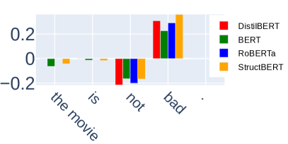
Fig. 4 shows local OSV( $\phi^{a}$ ) with marginal intervention with a single token [MASK], for all four models on two example instances. We observe an interesting distinction between the two: High $\phi(z)$ compared to $\phi(x)$ on not and bad across all models in Fig. 4c indicates that it is essential for not to precede bad to correctly reverse the sentiment. However $\phi(z)$ on not good (Fig. 4a), is comparably smaller in magnitude for all models, particularly for DistilBERT and BERT, where the attributions to order features are negligible. This discrepancy is mostly likely caused by the inherent polarity of the word not, hence models do not have to encode order for negating positive adjectives while order is essential for negating negative adjectives. Similar polarity of negation cues are also observed in prior works [43, 44], while OSV provides a more precise analytical approach to surface it. One possible reason for the model-wise difference is that RoBERTa and StructBERT benefit from their improved training procedures over BERT/DistilBERT. StructBERT, for example, is specially designed to be sensitive to word orders during pretraining.

To demonstrate the potential weakness of such order insensitivity of BERT and DistilBERT, we construct an adversarial dataset (REG*) by appending one of five neutral phrases containing negation words(not as expected, not like the other, not gonna lie, never gonna lie, never as expected), to the end of sentences of REG, effectively creating sentences such as The movie is good not gonna lie, which happens to contain the flipped negation construct(good not) and not in this context should not convey any sentiment. This dataset of size 7680 is evenly distributed between negative and positive sentiments. The result is shown in Tab. IV. Mirroring the difference in order-sensitivity shown by $\phi(z)$ , DistilBERT and BERT both suffer a 15% decrease for sentences with positive sentiments (REG*(+)) while the accuracy is either unchanged for RoBERTa and StructBERT, or decreases slightly for sentences with negative sentiments (REG*(-)) for all models. To further ensure the drop is not merely caused by the inherent negative sentiment of the word not (apart from the same $\phi(x)$ for not in Fig. 4a), we test two alternative datasets: (1) REG*, inserts a comma between the appended phrase and the original sentences, ex.: The movie is good, not gonna lie. (2) REG*B appends the phrases to the beginning of the sentences instead. Interestingly, all four models are robust to both alternatives. This distinction implies that the models are capable of disregarding the added phrases if negation cues are not directly proximate to the adjective. OSV, unlike SV, effectively surfaces local order-insensitivity in the negation construct, which is validated by BERT & DistilBERT’s failure on REG*(+).

TABLE V: Absolute-relative order discrepancy and Model performances for SVA.

	SVA-Obj			SVA-Subj
	$\Delta\phi^{z}_{su}$	Acc.*	Acc.	$\Delta\phi^{z}_{su}$	Acc.*	Acc.
DistilBERT	.04	.86( $\downarrow$ .05)	.91	.12	.79( $\downarrow$ .14)	.92
BERT-B	-.03	.93( $\downarrow$ .00)	.93	.11	.94( $\downarrow$ .04)	.99
BERT-L	-.05	.81( $\downarrow$ .00)	.81	.09	.92( $\downarrow$ .04)	.96
RoBERTa	-.04	.71( $\downarrow$ .00)	.71	.09	.64( $\downarrow$ .08)	.72

IV-B3 Subject-Verb Agreement(SVA)

While fine-tuned classification models may not learn word order because they don’t have to, a pretrained language model should, in theory, be more sensitive to order, especially when evaluated on syntactic tasks such as Subject-Verb Agreement. The task of SVA evaluates whether a language model prefers the correct verb form to match with the subject. For example, a pretrained masked language model should assign higher probability to is over are for the sentence The cat ¡mask¿ cute.

How language models learn SVA is widely studied in prior works [45, 46, 47]. In this section, we focus on two complicated long-range formulations of SVA where Transformers excel over simple RNN models [48]: SVA across subject relative clauses (SVA-subj) and SVA across object relative clauses (SVA-obj). For example, test instances for SVA-obj are generated from the template: the [Subject] that the [Attractor] [Verb] ¡mask?(is/are)¿ [Adjective].(ex.Fig. 5a). A language model needs to correctly parse the sentence to identify the true subject. In particular, when Attractor is of an opposite number to the Subject, a model that fails to parse the sentence will be distracted by the more proximate attractor. Prior works find that Transformer models succeed in long-range SVA and overcome such distraction because they learn composite syntactic structures [49, 50].

Models and Data

We use dataset from [51] and the cloze-style set up used in [48]. Specifically, we look at sentences with oppositely numbered attractors. We evaluate four pretrained langauge models: DistilBERT [41], BERT-Base & BERT-Large [6], and RoBERTa [17]. The accuracy of each task is found in Tab. V, where all models perform quite well except for RoBERTa, which still scores more than 70%.

Result

Fig. 5 show the global explanations for SVA-Obj and SVA-Subj with $f^{y}(x)=p_{correct\_verb}-p_{incorrect\_verb}$ and the same $g$ as Sec. IV-B1. We observe that the subject word exerts positive attribution on the correct choice of the verb, and the intervening noun (attractor) exerts negative attribution. In contrast to fine-tuned classification models such as NLI and SST, attributions to order features are high: they are indeed more important for syntactical tasks. Zooming in on the explanations, we obtain two other findings:

First, we observe that the relativizer word that is important as an order feature, but not as an occurrence feature. In other words, in order to predict the correct verb form, that itself may not contain the number signal, nevertheless it is regarded by the language model as an essential syntactic boundary.

Second, there is a big difference ( $\Delta\phi^{z}_{su}$ ) between $\phi^{a}$ and $\phi^{r}$ for the subject word in SVA-Subj., but not for SVA-Obj., i.e, the model seems to rely on absolute position of the subject word in SVA-Obj. much more than the relative position of the subject word. $\phi^{a}$ of the attractor is also much more negative than $\phi^{r}$ , indicating the model is distracted by the proximity of the attractor words (along with their occurrences). These distinctions point to a hypothesis that even though they contain exactly the same words, the model parses SVA-Obj. better than SVA-Subj., most likely due to the proximity of the attractor with ¡mask¿ in SVA-Subj. The higher accuracies of SVA-Obj. may be attributed to the models’ reliance on the absolute position of the subject words in the beginning of sentences, surfaced by the two modes of intervention on order features( $q^{a}$ & $q^{r}$ in Sec. III-C). Without attributing to order features, however, SV cannot uncover this subtle discrepancy.

To test this hypothesis, we create a simple adversarial set by prepending each of 23 punctuation and symbols¹¹1!”#&’*+,-./:<=>?@^_|~;<unk> such as “.” or <unk> to the beginning of sentences and see if such shifting of the subject from its absolute position impact the predictions. In Tab. V, Acc* shows all models suffer more from this adversarial perturbation for SVA-Subj than SVA-Obj, mirroring the distinction from $\Delta\phi^{z}_{su}$ . This indicates that the models’ learning of long-range SVA is not always conceptually sound, as is in the case of SVA-Subj..

V Related Work

Recent works [1, 2, 3, 4, 5, 52] show NLP models’ insensitivity to word orders. Our work corroborates such insensitivity by showing often insignificant attributions to order features in classification models. Meanwhile, a systematic explanation device such as OSV offers more precise and measurable attribution to the importance of order.

Shapley Values [10] is widely adopted as an model-agnostic explanation method [11, 12, 13, 14, 15] and also applied to explain text classification models [44, 53, 54]. However, the explanation power of these methods is limited by treating text data as tabular data. OSV, as demonstrated by numerous examples, allows us inspect the effect of “word occurrences” along side the effect of “word orders”. As order sensitivity is an essential metric of conceptual soundness, explanations incorporating order are more faithful in reflecting the true behavior of models.

We believe that explanations should not only function as a verification for plausibility [28], but also as a tool for diagnosing conceptual soundness. Instead of confirming the human understanding or the correct linguistic rules, explanations are equally, if not more, insightful when deviating from them. One popular approach to surface such deviation is adversarial examples [55], and many algorithms for finding them in NLP tasks [56, 57, 58] use gradient-based attributions such as saliency maps to guide adversarial perturbations. However, the use of orderless explanations is limited to local perturbations, such as swapping words into their synonyms. To allow for broader and non-local testing of model robustness, challenge datasets [59, 60, 61, 9] are constructed to stress test NLP models. These tests are becoming more crucial in designing and evaluating the conceptual soundness and robustness of NLP models beyond benchmark performances. However, rarely is the creation of those datasets guided by explanations methods, making it difficult to systematically and deductively discover non-local adversarial examples. In this paper, we show an initial attempt to bridge the gap between the two: we show that OSV not only informs on which, but how adversarial perturbations break models, enabling a deeper understanding of model weaknesses than orderless explanations. More broadly, the findings in Sec. IV-B echos [31] and [62], which discover that models learn “easier features”(e.g. occurrence features in HANS, not in SA and absolute order features in SVA) before learning “harder features” that may actually be the conceptually sound ones.

VI Conclusion

We propose OSV for explaining word orders of NLP models. We show how OSV is an essential extension of Shapley values and introduce two mechanisms for intervening on word orders. We highlight how OSV can precisely pinpoint if, where and how a model uses word order. Using adversarial examples guided by OSV, we demonstrate how order insensitivity, harmless as it seems, result in conceptually unsound models.

Acknowledgement

This work was developed with the support of NSF grant CNS-1704845. The U.S. Government is authorized to reproduce and distribute reprints for Governmental purposes not withstanding any copyright notation thereon. The views, opinions, and/or findings expressed are those of the author(s) and should not be interpreted as representing the National Science Foundation or the U.S. Government. We gratefully acknowledge the support of NVIDIA Corporation with the donation of the Titan V GPU used for this work.

References

[1] T. M. Pham, T. Bui, L. Mai, and A. Nguyen, “Out of order: How important is the sequential order of words in a sentence in natural language understanding tasks?” arXiv preprint arXiv:2012.15180, 2020.
[2] K. Sinha, R. Jia, D. Hupkes, J. Pineau, A. Williams, and D. Kiela, “Masked language modeling and the distributional hypothesis: Order word matters pre-training for little,” in Proceedings of the 2021 Conference on Empirical Methods in Natural Language Processing, 2021, pp. 2888–2913.
[3] L. Clouatre, P. Parthasarathi, A. Zouaq, and S. Chandar, “Demystifying neural language models’ insensitivity to word-order,” arXiv preprint arXiv:2107.13955, 2021.
[4] M. Alleman, J. Mamou, M. A. Del Rio, H. Tang, Y. Kim, and S. Chung, “Syntactic perturbations reveal representational correlates of hierarchical phrase structure in pretrained language models,” in Proceedings of the 6th Workshop on Representation Learning for NLP (RepL4NLP-2021), 2021, pp. 263–276.
[5] K. Sinha, P. Parthasarathi, J. Pineau, and A. Williams, “Unnatural language inference,” in Proceedings of the 59th Annual Meeting of the Association for Computational Linguistics and the 11th International Joint Conference on Natural Language Processing (Volume 1: Long Papers), 2021, pp. 7329–7346.
[6] J. Devlin, M.-W. Chang, K. Lee, and K. Toutanova, “Bert: Pre-training of deep bidirectional transformers for language understanding,” in Proceedings of the 2019 Conference of the North American Chapter of the Association for Computational Linguistics: Human Language Technologies, Volume 1 (Long and Short Papers), 2019, pp. 4171–4186.
[7] N. Malkin, S. Lanka, P. Goel, and N. Jojic, “Studying word order through iterative shuffling,” in Proceedings of the 2021 Conference on Empirical Methods in Natural Language Processing, 2021, pp. 10 351–10 366.
[8] P. M. Parkinson, “Sr 11-7: Guidance on model risk management,” Board of Governors of the Federal Reserve System, 20th Street NW, Washington, DC, vol. 20551, 2011.
[9] T. McCoy, E. Pavlick, and T. Linzen, “Right for the wrong reasons: Diagnosing syntactic heuristics in natural language inference,” in Proceedings of the 57th Annual Meeting of the Association for Computational Linguistics, 2019, pp. 3428–3448.
[10] L. S. Shapley, H. Kuhn, and A. Tucker, “Contributions to the theory of games,” Annals of Mathematics studies, vol. 28, no. 2, pp. 307–317, 1953.
[11] E. Strumbelj and I. Kononenko, “An efficient explanation of individual classifications using game theory,” The Journal of Machine Learning Research, vol. 11, pp. 1–18, 2010.
[12] A. Datta, S. Sen, and Y. Zick, “Algorithmic transparency via quantitative input influence: Theory and experiments with learning systems,” in 2016 IEEE symposium on security and privacy (SP). IEEE, 2016, pp. 598–617.
[13] S. M. Lundberg and S.-I. Lee, “A unified approach to interpreting model predictions,” in Proceedings of the 31st international conference on neural information processing systems, 2017, pp. 4768–4777.
[14] M. Sundararajan and A. Najmi, “The many shapley values for model explanation,” in International Conference on Machine Learning. PMLR, 2020, pp. 9269–9278.
[15] I. Covert, S. M. Lundberg, and S.-I. Lee, “Understanding global feature contributions with additive importance measures,” Advances in Neural Information Processing Systems, vol. 33, 2020.
[16] J. Min, R. T. McCoy, D. Das, E. Pitler, and T. Linzen, “Syntactic data augmentation increases robustness to inference heuristics,” in Proceedings of the 58th Annual Meeting of the Association for Computational Linguistics, 2020, pp. 2339–2352.
[17] Y. Liu, M. Ott, N. Goyal, J. Du, M. Joshi, D. Chen, O. Levy, M. Lewis, L. Zettlemoyer, and V. Stoyanov, “Roberta: A robustly optimized bert pretraining approach,” arXiv preprint arXiv:1907.11692, 2019.
[18] W. Wang, B. Bi, M. Yan, C. Wu, J. Xia, Z. Bao, L. Peng, and L. Si, “Structbert: Incorporating language structures into pre-training for deep language understanding,” in International Conference on Learning Representations, 2019.
[19] I. Covert, S. Lundberg, and S.-I. Lee, “Explaining by removing: A unified framework for model explanation,” Journal of Machine Learning Research, vol. 22, no. 209, pp. 1–90, 2021.
[20] H. Chen, J. D. Janizek, S. Lundberg, and S.-I. Lee, “True to the model or true to the data?” arXiv preprint arXiv:2006.16234, 2020.
[21] I. E. Kumar, S. Venkatasubramanian, C. Scheidegger, and S. Friedler, “Problems with shapley-value-based explanations as feature importance measures,” in International Conference on Machine Learning. PMLR, 2020, pp. 5491–5500.
[22] A. Catav, B. Fu, Y. Zoabi, A. L. W. Meilik, N. Shomron, J. Ernst, S. Sankararaman, and R. Gilad-Bachrach, “Marginal contribution feature importance-an axiomatic approach for explaining data,” in International Conference on Machine Learning. PMLR, 2021, pp. 1324–1335.
[23] C. Frye, D. de Mijolla, T. Begley, L. Cowton, M. Stanley, and I. Feige, “Shapley explainability on the data manifold,” in International Conference on Learning Representations, 2020.
[24] P. Hase, H. Xie, and M. Bansal, “The out-of-distribution problem in explainability and search methods for feature importance explanations,” Advances in Neural Information Processing Systems, vol. 34, 2021.
[25] J. F. Banzhaf III, “Weighted voting doesn’t work: A mathematical analysis,” Rutgers L. Rev., vol. 19, p. 317, 1964.
[26] M. T. Ribeiro, S. Singh, and C. Guestrin, “” why should i trust you?” explaining the predictions of any classifier,” in Proceedings of the 22nd ACM SIGKDD international conference on knowledge discovery and data mining, 2016, pp. 1135–1144.
[27] M. Ancona, C. Oztireli, and M. Gross, “Explaining deep neural networks with a polynomial time algorithm for shapley value approximation,” in International Conference on Machine Learning. PMLR, 2019, pp. 272–281.
[28] A. Jacovi and Y. Goldberg, “Towards faithfully interpretable nlp systems: How should we define and evaluate faithfulness?” in Proceedings of the 58th Annual Meeting of the Association for Computational Linguistics, 2020, pp. 4198–4205.
[29] Y. Ju, Y. Zhang, Z. Yang, Z. Jiang, K. Liu, and J. Zhao, “The logic traps in evaluating post-hoc interpretations,” arXiv preprint arXiv:2109.05463, 2021.
[30] Y. Zhou, S. Booth, M. T. Ribeiro, and J. Shah, “Do feature attribution methods correctly attribute features?” arXiv preprint arXiv:2104.14403, 2021.
[31] C. Lovering, R. Jha, T. Linzen, and E. Pavlick, “Predicting inductive biases of pre-trained models,” in International Conference on Learning Representations, 2020.
[32] S. Hochreiter and J. Schmidhuber, “Long short-term memory,” Neural computation, vol. 9, no. 8, pp. 1735–1780, 1997.
[33] A. Vaswani, N. Shazeer, N. Parmar, J. Uszkoreit, L. Jones, A. N. Gomez, u. Kaiser, and I. Polosukhin, “Attention is all you need,” in Proceedings of the 31st International Conference on Neural Information Processing Systems, 2017.
[34] K. Leino, S. Sen, A. Datta, M. Fredrikson, and L. Li, “Influence-directed explanations for deep convolutional networks,” in 2018 IEEE International Test Conference (ITC). IEEE, 2018.
[35] K. Simonyan, A. Vedaldi, and A. Zisserman, “Deep inside convolutional networks: Visualising image classification models and saliency maps,” in Workshop at International Conference on Learning Representations, 2014.
[36] M. Sundararajan, A. Taly, and Q. Yan, “Axiomatic attribution for deep networks,” in Proceedings of the 34th International Conference on Machine Learning-Volume 70, 2017.
[37] A. Williams, N. Nangia, and S. Bowman, “A broad-coverage challenge corpus for sentence understanding through inference,” in Proceedings of the 2018 Conference of the North American Chapter of the Association for Computational Linguistics: Human Language Technologies, Volume 1 (Long Papers), 2018, pp. 1112–1122.
[38] Y. Yaghoobzadeh, S. Mehri, R. T. des Combes, T. J. Hazen, and A. Sordoni, “Increasing robustness to spurious correlations using forgettable examples,” in Proceedings of the 16th Conference of the European Chapter of the Association for Computational Linguistics: Main Volume, 2021, pp. 3319–3332.
[39] K. Lu, P. Mardziel, F. Wu, P. Amancharla, and A. Datta, “Gender bias in neural natural language processing,” arXiv preprint arXiv:1807.11714, 2018.
[40] R. Jha, C. Lovering, and E. Pavlick, “Does data augmentation improve generalization in nlp?” arXiv preprint arXiv:2004.15012, 2020.
[41] V. Sanh, L. Debut, J. Chaumond, and T. Wolf, “Distilbert, a distilled version of bert: smaller, faster, cheaper and lighter,” arXiv preprint arXiv:1910.01108, 2019.
[42] A. Wang, A. Singh, J. Michael, F. Hill, O. Levy, and S. Bowman, “Glue: A multi-task benchmark and analysis platform for natural language understanding,” in Proceedings of the 2018 EMNLP Workshop BlackboxNLP: Analyzing and Interpreting Neural Networks for NLP, 2018, pp. 353–355.
[43] K. Lu, Z. Wang, P. Mardziel, and A. Datta, “Influence patterns for explaining information flow in bert,” Advances in Neural Information Processing Systems, vol. 34, 2021.
[44] J. Chen and M. Jordan, “Ls-tree: Model interpretation when the data are linguistic,” in Proceedings of the AAAI Conference on Artificial Intelligence, vol. 34, no. 04, 2020, pp. 3454–3461.
[45] T. Linzen, E. Dupoux, and Y. Goldberg, “Assessing the ability of lstms to learn syntax-sensitive dependencies,” Transactions of the Association for Computational Linguistics, 2016.
[46] K. Lu, P. Mardziel, K. Leino, M. Fredrikson, and A. Datta, “Influence paths for characterizing subject-verb number agreement in LSTM language models,” in Proceedings of the 58th Annual Meeting of the Association for Computational Linguistics. Association for Computational Linguistics, 2020.
[47] J. Wei, D. Garrette, T. Linzen, and E. Pavlick, “Frequency effects on syntactic rule learning in transformers,” in Proceedings of the 2021 Conference on Empirical Methods in Natural Language Processing, 2021, pp. 932–948.
[48] Y. Goldberg, “Assessing bert’s syntactic abilities,” arXiv preprint arXiv:1901.05287, 2019.
[49] G. Jawahar, B. Sagot, and D. Seddah, “What does bert learn about the structure of language?” in Proceedings of the 57th Annual Meeting of the Association for Computational Linguistics, 2019.
[50] J. Hewitt and C. D. Manning, “A structural probe for finding syntax in word representations,” in Proceedings of the 2019 Conference of the North American Chapter of the Association for Computational Linguistics: Human Language Technologies, Volume 1 (Long and Short Papers), 2019.
[51] R. Marvin and T. Linzen, “Targeted syntactic evaluation of language models,” in Proceedings of the 2018 Conference on Empirical Methods in Natural Language Processing, 2018.
[52] A. Gupta, G. Kvernadze, and V. Srikumar, “Bert & family eat word salad: Experiments with text understanding,” 2021.
[53] D. Zhang, H. Zhou, H. Zhang, X. Bao, D. Huo, R. Chen, X. Cheng, M. Wu, and Q. Zhang, “Building interpretable interaction trees for deep nlp models,” in Proceedings of the AAAI Conference on Artificial Intelligence, vol. 35, no. 16, 2021, pp. 14 328–14 337.
[54] J. Chen, L. Song, M. J. Wainwright, and M. I. Jordan, “L-shapley and c-shapley: Efficient model interpretation for structured data,” in International Conference on Learning Representations, 2018.
[55] W. E. Zhang, Q. Z. Sheng, A. Alhazmi, and C. Li, “Adversarial attacks on deep-learning models in natural language processing: A survey,” ACM Transactions on Intelligent Systems and Technology (TIST), vol. 11, no. 3, pp. 1–41, 2020.
[56] M. Cheng, J. Yi, P.-Y. Chen, H. Zhang, and C.-J. Hsieh, “Seq2sick: Evaluating the robustness of sequence-to-sequence models with adversarial examples,” in Proceedings of the AAAI Conference on Artificial Intelligence, vol. 34, no. 04, 2020, pp. 3601–3608.
[57] J. Ebrahimi, A. Rao, D. Lowd, and D. Dou, “Hotflip: White-box adversarial examples for text classification,” arXiv preprint arXiv:1712.06751, 2017.
[58] E. Wallace, S. Feng, N. Kandpal, M. Gardner, and S. Singh, “Universal adversarial triggers for attacking and analyzing nlp,” in Proceedings of the 2019 Conference on Empirical Methods in Natural Language Processing and the 9th International Joint Conference on Natural Language Processing (EMNLP-IJCNLP), 2019, pp. 2153–2162.
[59] Y. Belinkov, N. Durrani, F. Dalvi, H. Sajjad, and J. Glass, “What do neural machine translation models learn about morphology?” in Proceedings of the 55th Annual Meeting of the Association for Computational Linguistics (Volume 1: Long Papers), 2017, pp. 861–872.
[60] M. T. Ribeiro, T. Wu, C. Guestrin, and S. Singh, “Beyond accuracy: Behavioral testing of nlp models with checklist,” in Proceedings of the 58th Annual Meeting of the Association for Computational Linguistics, 2020, pp. 4902–4912.
[61] T. Wu, M. T. Ribeiro, J. Heer, and D. S. Weld, “Polyjuice: Generating counterfactuals for explaining, evaluating, and improving models,” in Proceedings of the 59th Annual Meeting of the Association for Computational Linguistics and the 11th International Joint Conference on Natural Language Processing (Volume 1: Long Papers), 2021, pp. 6707–6723.
[62] K. Mangalam and V. U. Prabhu, “Do deep neural networks learn shallow learnable examples first?” 2019.
[63] T. Wolf, L. Debut, V. Sanh, J. Chaumond, C. Delangue, A. Moi, P. Cistac, T. Rault, R. Louf, M. Funtowicz et al., “Huggingface’s transformers: State-of-the-art natural language processing,” arXiv preprint arXiv:1910.03771, 2019.

Appendix A Code and Data

Code is included in the supplementary material. Data for SA is introduced in Appendix F while all other data in Sec. IV-B are publicly available as benchmark datasets. The code for synthesizing the data in Sec. IV-A is included in the code files.

Appendix B Proof of Remark 1 and Axiomatic Interpretations of OSV

B-A Proof of remark 1

An alternative definition[12] for $\phi^{z}_{f^{y}}(i)$ is:

	$\displaystyle\forall x_{i}\in x,\phi^{z}_{f^{y}}(x_{i})$	$\displaystyle=\frac{1}{(2n)!}\sum_{\sigma\subseteq\Pi(N^{\prime})}m_{i}(\sigma)$
		$\displaystyle=\frac{1}{(2n)!}\cdot\frac{(2n)!}{n!}\sum_{\sigma\subseteq\Pi(N)}m_{i}(\sigma)$
		$\displaystyle=\frac{1}{n!}\sum_{\sigma\subseteq\Pi(N)}m_{i}(S)$
		$\displaystyle=\phi_{f^{y}}(x_{i})$
	$\displaystyle where:m_{i}(\sigma)$	$\displaystyle=m\left(P_{i}(\sigma)\right)$
	$\displaystyle P_{i}(\sigma)$	$\displaystyle=\{j\mid\sigma_{j}<\sigma_{i}\}$

$P_{i}$ is the set of $i$ ’s predecessors in $\sigma$ . $\forall z_{i}\in z$ , according to the dummy axiom, since $z$ is omnipresent, $f^{y}(S\cup i)=f^{y}(S)$ , so $\phi^{z}_{f^{y}}(z_{i})=0,\forall z_{i}\in z$ .

B-B Axioms of Shapley Values

The axiomatic properties of Shapley values are first introduced in [10] and extensively discussed in the context of machine learning in [13] and [12]. Shapley values defined in Eq. 1 is the only value satisfying all following axioms. The names in parenthesis are alternative names used in literature.

Symmetry Axiom

$i,j\in N$ are symmetric if $v(S\cup i)=v(S\cup j)$ for all $S\subseteq N\backslash{i,j}$ . A value $\phi$ satisfies symmetry if $\phi(i)=\phi(j)$ whenever $i$ and $j$ are symmetric.

Extending to order features, if two order features are symmetric, meaning that their positions are always interchangeable, then their attributions should equal each other. Though theoretically possible, order features are unlikely to be symmetric with occurrence features.

Dummy Axiom(Null Effects/Missingness)

A player is a dummy or null player if $v(S\cup i)=v(S)$ for all $S\subseteq N$ . A value $\phi$ satisfies the dummy axiom if $\phi(i)=0$ whenever $i$ is a dummy or null player.

An order feature is a dummy: (1) if the model doesn’t care where it is in a model, for example a BoW model; (2) if the order feature is omnipresent as in Remark 1.

Completeness Axiom (Efficiency or Local Accuracy)

A value $\phi$ satisfies completeness if $\sum_{i}^{N}\phi(i)=v(N)$ . This axiom is important as it makes Shapley value an attribution value in that it attributes and allocates the output of the function to individual inputs.

Monoticity Axiom (Consistency)

A value $\phi$ satisfies monoticity if $m(S,v_{1})\geq m(S,v_{2})$ for all $S$ implies that $\phi_{v_{1}}(i)\geq\phi_{v_{2}}(i)$ . The theorem of monoticity states that if one features’ contribution is greater for one model than another model regardless of all other inputs, that input’s attribution should also be higher. It can be extended directly to order features.

Appendix C Implementation details

To make sure that the global explanations truly represent the global contribution of each feature towards the prediction, we use a convergence factor of $t=0.005$ for all global explanations, meaning the variance of the Shapley value is less than $0.5\%$ of the difference between the maximum and minimum $\phi(i)$ for all $i$ (a looser $t=0.01$ is sufficient for convergence according to [15]). For each $S$ , we use a sample size of 4 for $q$ and a sample size of 5 for $g$ when $g$ samples from templates (total of 20 intervened sentences per instance per $S$ ). We find this setting generates stable explanations for the synthetic data (low variance in Tab. II). Moreover, since the stopping condition is based on $t$ and the algorithm for computing global explanations may iterate through the whole data multiple times to reach that convergence, the actual sample size of $q$ and $g$ in principle should not matter.

For StructBERT [18] and $M_{for}$ of Sec. IV-B1, we use the implementation from the official repositories. For other models including $M_{aug}$ of Sec. IV-B1, we either use models available in the Huggingface [63] repository or fine-tuned each model with 3 epochs using the default parameters of HuggingFace Trainer class. We do not make extensive efforts to tune the hyperparameters since the goal of this paper is not to use the best models but to show the utility of an explanation device.

Tab. VI shows the average number of evaluations (number of intervened instances) per instance for computing global explanations shown in Fig. 2 and 6. For sequences of length 8, $\phi^{z}$ needs less than 8 times more evaluation for convergence, corroborating Theorem 2 of [15].

Depending on the length of the sequence, GPU run time on a for computing OSV varies. In this paper, all experiments finish with a reasonable amount of time even with the tight convergence setting. For example, on average, each template in Sec. IV-B1 takes around 5 min.

TABLE VI: Average (across 25 seeds) number of evaluations per instance for synthetic experiments

	LSTM	Transformer
$\phi^{a}$	2425	2299
$\phi^{r}$	2485	2445
$\phi$	330	331

Appendix D Additional Results for Sec. IV-A

For IG, we use 1000 as the number of steps for approximation(the authors of IG recommends 20 to 1000 steps). The model performance and explanation visualizations for transformer models are included in Tab. VII and Fig. 6.

TABLE VII: Tasks Description and Model performances for Synthetic Data Experiments for transformer models. Acc. are test accuracies for each model over 5 random seeds, Acc-1 are accuracies for

[\mathbf{W_{1}}]

Ind.	Condition for y=1	Acc.	Acc-1.
1	Begins with duplicate	1.00 $\pm$ .00	1.00 $\pm$ .00
2	Adjacent duplicate	0.98 $\pm$ .00	0.99 $\pm$ .01
3	Any duplicate	1.00 $\pm$ .00	1.00 $\pm$ .00

Appendix E Additional Results for HANS (Sec. IV-B1)

We compute the global explanations for all templates in [9], where half of the templates is labeled as entailment. For those templates, word overlapping heuristics is actually the correct heuristic for predicting entailment. Tab. VIII shows the same stats as Tab. III, but for entailment-labeled templates. As we can see, $M_{for}$ is actually less order-sensitive than $M_{aug}$ . Ideally, a conceptually sound model should learn both word overlaps and word orders; nevertheless this discrepancy can also be explained by overfitting and mere shifting of decision boundary: $M_{aug}$ only learn that word overlap at the corresponding positions does not equate to entailment, making the model more order-sensitive for entailment-labeled sentences. While $M_{for}$ also rely on word-overlapping features much more than order, but possibly in the same way as $M_{ori}$ .

TABLE VIII: Global Statistics across entailment-labeled templates

	$\sum_{i}\phi(x_{i})$	$\sum_{i}\phi(z_{i})$
$M_{ori}$	1.26	-0.37
$M_{aug}$	0.85( $\downarrow$ 0.41)	-0.09( $\uparrow$ 0.28)
$M_{for}$	0.89( $\downarrow$ 0.37)	-0.22( $\uparrow$ 0.15)

Appendix F Additional Details for SA (Sec. IV-B2)

F-A Templates for NEG/REG

[Det(The)] [Noun(movie)] [Verb(is)] [NEG/REG] [Adjective(good)][(Punc).]

•

Det: ’the’, ’that’, ’this’, ’a’
•

Noun: ’film’, ’movie’, ’work’, ’picture’
•

Verb: ’is’, ’was’
•

NEG: ’not’, ’never’, ’not that’, ’never that’
•

REG: ”(blank), ’very’, ’pretty’, ’quite’
•

Adjective: (+): ’good’, ’amazing’, ’great’
•

Adjective: (-): ’boring’, ’bad’, ’disappointing’
•

Punctuations: ’.’, ’!’

F-B Aggregated Results for Fig. 4

We compute the aggregated global explanations for all instances of NEG(+) and NEG(-), illustrated in Fig. 7, to make sure the trend shown in Fig. 4 represent the general trend. In Fig. 8, we show local explanations for a sentence in REG with no special construct like negation, and as expected, word orders do not matter at all.