Orbital angular momentum due to modes interference
Abstract
We present generalized expressions to calculate the orbital angular momentum for invariant beams using scalars potentials. The solutions can be separated into transversal electric TE, transversal magnetic TM and transversal electromagnetic TE/TM polarization modes. We show that the superposition of non-paraxial vectorial beams with axial symmetry can provide a well defined orbital angular momentum and that the modes superposition affects the angular momentum flux density. The results are illustrated and analyzed for Bessel beams.
1 Introduction
Since the pioneering and interesting work of the orbital angular momentum presented by L. Allen [1], the study of the subject have covered many interesting applications [2]; a compilation overview over the last 25 years, with several theoretical and experimental applications was reported in [3]. The authors in [4] have recently demonstrated that a rotationally arranged nano-antenna can be used to convert the phase information in a twisted light beam into spectral information, which hence can be used to classify the phase state of the twisted light beam. This effect has strong influence on the optical properties of dielectric and plasmonic particles and it is useful for new technological applications. The physical properties of the orbital angular momentum have the potential to improve the performance of optical communication systems in different ways [5], but it is not the aim of this manuscript to explore the full list of possibilities. Exploiting the physical properties of the orbital angular momentum is the subject of an increasing number of research topics nowadays. In this context, here we focus in the use of the scalar formalism for studying the orbital angular momentum for invariant beams; due to its simplicity, this approach has been theoretically [6] and experimentally [7, 8] used and tested.
Recently, the scalar representation has been used to describe scattering problems using partial waves series in the far field approximation, where the impinging source is a structured field [9]. Effects also considering the polarization [10], the extinction [11] and driven acoustic radiation forces [12] have also been considered. Furthermore, the scalar approach is a natural representation for the structured beams family, also known as “non-diffracting beams”. The study of these fields covers different areas, from quantum mechanics to astrophysics [13]. Such fields are the Bessel [14], Mathieu [15] and Weber beams [16], which are constructed by superposition of plane-waves [17], formalism which is called angular spectrum representation [18]. These ideal fields propagate indefinitely without changing their transverse intensity distribution [19], even in the presence of massive phase perturbations and into inhomogeneous media [20]. As an interesting application, among others, this physical effect increases the resolution and contrast to image sub-cellular components and organelles in different microscopy methods [21].
Otherwise, the study of structured invariant beams is of increasing interest in optical physics. Their properties make them particularly attractive for optical design [22], for studying propagation through etalons and crystals [23]. Another interesting example is the use of Bessel beams for driving an optimal single tractor beam for dielectric particles with cylindrical shape [24].
The study of nonparaxial orbital angular momentum was recently revisited in [25] using Bessel beams; in that work, the authors show well defined orbital angular momentum properties, without considering the possibility of contributions due to mixed modes superimposed along their propagation. To the best of our knowledge, this feature has not been fully explored. However, recently, using the scalar potential approach, fundamentals electromagnetic properties, such as the energy density, the Poynting vector, the Maxwell stress tensor for nonparaxial beams were derived [26]. Currently, the study of the Poynting vector has been taken considerable interest due to its features and properties along the propagation.
In the context of structured beams, Novitsky in [27] has shown that Bessel beams possess negative values in the longitudinal and azimuthal components of the Poynting vector, which depends in the superposition of mixed modes and on the phase detuning between the complex amplitudes and of the transversal electric or magnetic part of the beam representation. Since then, many interesting results have been reported, such as the explanation of optical pulling forces [28], effects in meta-materials [29], tractor beams [30] and optical manipulation [31], to name a few of them. Another interesting case was reported for X-Waves in [32], where the propagation direction of their negative Poynting vector could be locally changed using carefully chosen complex amplitudes; however, we showed [26] that the negative behavior can be found independently of the mode interference. Nonetheless, the Poynting vector behavior presented in the Bessel beams and in the X-Waves, mentioned above, has opened a discussion related to tractor beams generation, and with other interesting applications, such as the forces that can be locally oriented in a direction opposite to the propagation wave vector [33].
Then, what is the relationship between mixed modes and the Negative Poynting Vector (NPV)? This effect can be physically defined as an uncommon response produced by the local sign change in the Poynting vector components along its propagation. Recently, we reported in [34] to deep in the understanding of the NPV to study the invariant family beams. The main result of our work was to show the negative local change of the negative Poynting vector, which can be independently obtained without to superposition of mixed modes TE/TM, as it is in the case of Weber beams [34]. Additionally, considerable interest in theoretically and experimentally studies of the vectorial structured fields are driven by the possibility to create a wide variety of exotic optical focal fields with homogeneous and spatially inhomogeneous states of polarization; an interesting review of the wide scope of interest and applications is presented in [35].
In this context, the study of the properties of the orbital angular momentum from the theoretical an experimental points of view can open new engineering technologies. Using the concept of the Poynting vector can be useful, as shown by proposals to measure the orbital angular momentum using superposition of vector mixed modes TE/TM. This was performed and tested for a Laguerre Gauss beams [36]. This approach may open interest for other structured fields, as it was also proposed by using waves in ultrashort optical pulses [37]. Even, in the case of two electromagnetic plane waves with the same angular frequency and different wave vectors, the superposition fields reveals highly nontrivial structure in the local momentum and spin densities [38], that can be used to enhance the optical manipulations of small particles. For example, the spinning dynamics can be driven by superposing two vortex beams with respective circular and radial polarizations such that the particle spins around a certain optical axis [39]. The authors in [40, 41] have pointed out the importance of the Poynting vector for obtaining orbital angular momentum from spatial superposition of the Poynting vector beams.
This article is organized as follows: in Section 2, we briefly review the theoretical framework based on the scalar potential approach; in Section 3, we present the general negative Poynting vector for the whole invariant beams family; in Section 4, we study the orbital angular momentum in their transversal and longitudinal propagation due to mixed modes and in Section 5, we present our conclusions.
2 Maxwell equations in terms of scalar potentials
Following the formalism proposed by Stratton [42], we write the electromagnetic fields as
| (1a) | ||||
| (1b) | ||||
where and are vector fields proposed as
| (2) |
and
| (3) |
being a scalar field, an arbitrary unit vector that determines the direction of propagation (which we will choose as the axis, so ), the magnitude of the wave vector, the electric permittivity, the magnetic permeability, and and two arbitrary complex numbers. This approach has been successfully used to study the properties of the family of invariant beams, theoretically and experimentally [6, 7, 8].
It is straightforward to verify that if a scalar field satisfies the Helmholtz equation
| (4) |
then the fields (1a) and (1b) satisfy the Maxwell equations; so, the scalar field will be named scalar potential. Note that the vector fields, and , are orthogonal, that is , and solenoidal, i.e. and .
On the other hand, for any invariant beam the spatial evolution of the scalar potential can be described by its transverse and longitudinal parts [43]. The transverse part will depend only on the transverse coordinates, , and the longitudinal part will depend on the longitudinal coordinate (as we selected ), physically the propagation axis; i.e., we can write
| (5) |
After substituting (5) in the Helmholtz equation, we easily obtain that satisfies the two dimensional transverse Helmholtz equation
| (6) |
where is the Laplacian transversal operator, which has a specific form in each coordinate system, and the longitudinal part is with the dispersion relation . The two dimensional transverse Helmholtz equation (6) can be separated in Cartesian, cylindrical, parabolic cylindrical and elliptical cylindrical coordinates [43], and that gives origin to plane waves, Bessel beams, Weber beams and Mathieu beams, respectively. Then, we can write the vector operator fields, Eqs. (2) and (3), as follows
| (7) |
where
| (8) |
and are the base unit vectors corresponding to the transversal direction, and and are the corresponding scale factors. We note that in the four coordinate systems, in which equation (6) can be separated, the scale factor is equal to 1. It is also easy to verify that
| (9) |
where is the transversal part of the operators, i.e.
| (10) |
It is worth to notice that the transversal vector operators are related as follows .
3 A generalized Poynting vector for scalars potentials
The Poynting vector represents the directional power flux per unit area of an electromagnetic field. For harmonic electromagnetic fields the time average of the Poynting vector is given by [44]
| (11) |
Substituting expressions (1a) and (1b) for the electromagnetic fields into (11), a generalized expression for the Poynting vector of any invariant beam is obtained [26],
| (12) |
where
| (13) |
is the transversal electric part,
| (14) |
is the transversal magnetic part, and the interference modes TE/TM
| (15) |
The time averaged Poynting vector is independent of the coordinate and it satisfies , as was proven in [45]. It is important to remark that the interference term in the Poynting vector, expressed in Eq. (15), is different from zero for any invariant beam, of course, whenever at least one of the two constants and is not null. Physically this confirms the negative behavior trough the propagation; these results were recently reported in [34] using the Weber beams. The study of its effect on the orbital angular momentum is done in the following sections.
4 Orbital angular momentum density
For harmonic electromagnetic fields, the time averaged linear momentum per unit volume carried is [44, 50], and then, the time averaged orbital angular momentum density is ; using Eqs. (13), (14) and (15), we can find explicitly the contributions from the transverse electric, from the transverse magnetic and from the transverse electric/transverse magnetic TE/TM mixed modes. The transversal electric TE part is
| (16) |
whereas the transversal magnetic TM contribution has the form
| (17) |
and the interference mixed modes TE/TM part is given by
| (18) |
The set of equations (16), (17) and (18) provide a useful simple recipe to calculate the orbital angular momentum of any invariant beam in terms of scalar potentials. It is important to remark that Eq. (18) physically represents the orbital angular momentum propagation due to the superposition of modes TE/TM.
4.1 Example: orbital angular momentum for Bessel beams using a scalar potential
The properties of the orbital angular momentum have been extensively investigated by different means [3, 46]. However, to the best of our knowledge, the study of the orbital angular momentum arising from mode superposition has not been attempted before; nevertheless, the interference Bessel beams have been applied in the micro-manipulation of particles [47, 51]. With this in mind, and as an illustrative example, we analyze the particular case of the orbital angular momentum of Bessel beams.
The transversal solution of the scalar Helmholtz equation in cylindrical coordinates is
| (19) |
where is any integer, is the Bessel function of the first kind of order , and is the transversal vector [13]. Substituting (19) in (16), (17) and (18), we obtain the orbital angular momentum of a Bessel beam. The radial angular momentum is
| (20) |
while the azimuthal angular momentum component is
| (21) | ||||
and the longitudinal component is
| (22) |
As can be observed, all terms have a clear contribution of modes superposition, which in general is different from zero. Even, for the most simple case, when the azimuthal value is zero, , the mixed modes are given by
| (23) |
| (24) |
| (25) |
If the mixing is considered, these results show that there is interference between the radial and azimuthal components. Writing and , we have ; thus this term contribute if there is a difference of phase between and , otherwise this term is zero. Therefore, all the well-know results for the orbital angular momentum can be obtained.
4.2 Longitudinal orbital angular momentum
The above equations allow us to obtain the longitudinal orbital angular momentum for a particular transversal electric, magnetic or interference mode; the procedure is just to take the scalar product of (16), (17) and (32) with . For any invariant beams the longitudinal orbital angular momentum can be obtained as
| (26) |
| (27) |
| (28) |
where and . Where is given by Eq. (8) and which physically means a rotation of . Note that only the transversal structure beam, which is given for a single scalar potential , is required; all terms are proportional to . The equation (28) is given in terms of mixed modes and it is proportional to the ratio . In the particular case of the Bessel beams, we substitute expression (19) into (26) and (27) obtaining the following results
| (29) |
and
| (30) |
We have obtained a well-known defined orbital angular momentum; these results recover the results reported in [25] for Bessel beams. A well defined longitudinal orbital angular momentum is obtained for TE and TM modes when , since there is no orbital angular momentum in the direction of propagation; if , the beam carries orbital angular momentum in the direction of propagation [2, 3]. Additionally, using the Eq. (29), Eq. (30) and the longitudinal electromagnetic energy density reported in [26], it is straightforward to verify that the ratio of [25]. These results confirm a well-defined values of angular momentum and energy for this nonparaxial approximation.
For the case of longitudinal mixed modes, substituting (19) into (28) and after some algebraic manipulation, we get
| (31) |
In this more general case, the longitudinal orbital angular momentum is not proportional to the topological charge , as in the single mode case.
Now it is related to the radial derivative of the square field weighted by its radius minus the intensity of the incident field.
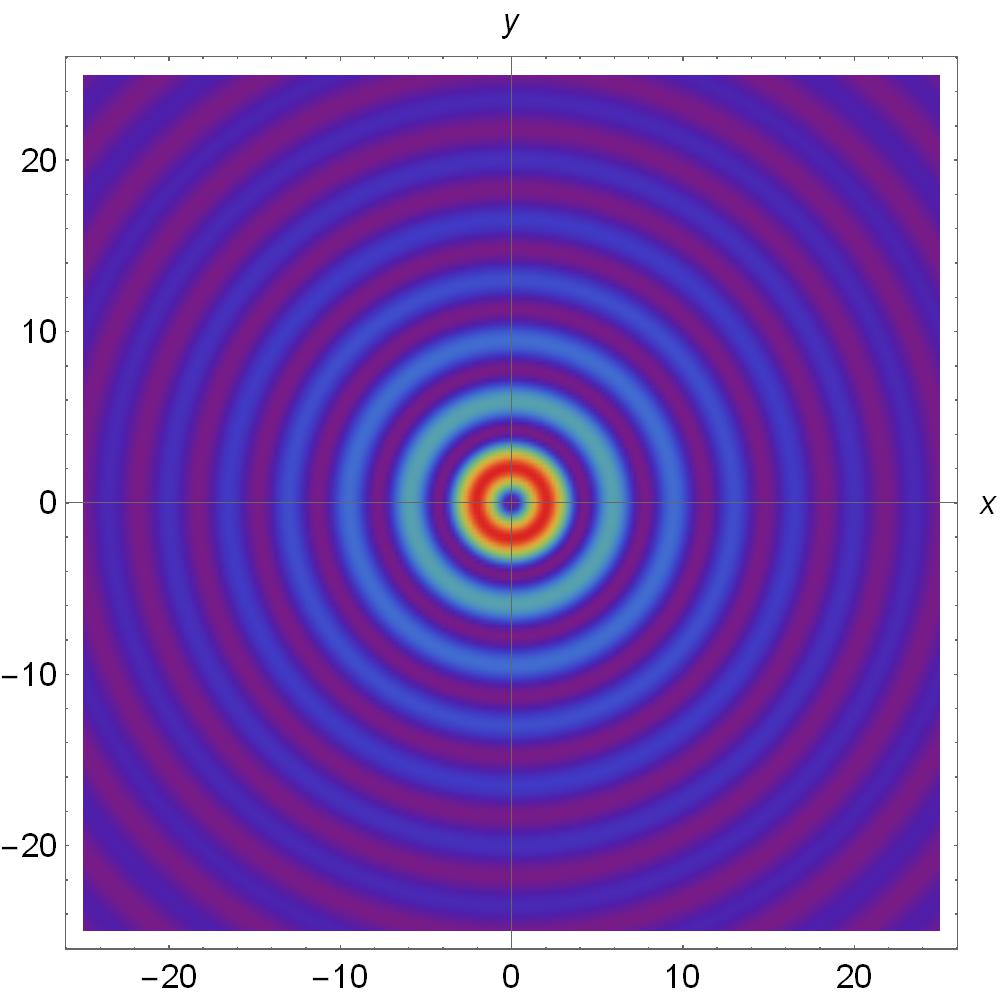
In Fig. 1, it is shown the transverse electric and the transverse magnetic longitudinal orbital angular momentum for Bessel beams with and .
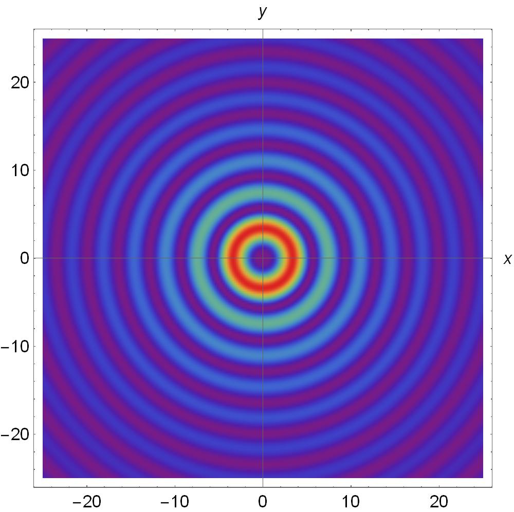
In Fig. 2 the mixed modes superposition longitudinal orbital angular momentum is shown for and for . We obtain a well-defined regions due to the interference superposition modes can be observed. This feature can be useful; the application of Bessel beams for optical manipulation has been proposed [47], and it has recently been successfully developed for the case of a single-beam or counter-propagating beam trapping [52].
Recently, in [53], it has been shown how combining two Bessel beams, as in equation (19), with topological charges , it is possible to generate a Hermite-Gauss (HG) beam, which posses well defined orbital angular momentum [54]. Moreover, it is important to mention that a superposition of Hermite-Gauss beams can be transformed into a Laguerre-Gauss beam [55] which posses a very well-know and characteristic factor [1, 2, 3]. Thus, our generalized analytical formulation makes possible the study the orbital angular momentum using a single scalar potential.
4.3 The transversal interference term carry orbital angular momentum
We can finally consider the paraxial approximation; i.e., the case when . We substitute that approximation into equation (32), in which the second term vanishes. Without loss of generality, we can rewrite the complex constants defined above as and . Then, it is straightforward to obtain
| (32) |
and
| (33) |
This expression clearly shows the vectorial transversal structure propagating due to mixed modes for any invariant beam. It is worth noticing the presence of the term , which is due to the fact that any invariant beam can be generated as a superposition of plane waves [18]. This parameter has been physically linked with polarization states and it has been usually reported in paraxial and nonparaxial approximations [2, 3]. After substituting a Bessel beam expressed by (19) into (33) and changing into cylindrical coordinates and , we obtain
| (34) |
This expression reveals that the orbital angular momentum contribution of the mixed modes is proportional to the topological azimuthal factor and depends linearly of the transversal wave vector. Taking means linear polarization and the lack of possible interference modes; otherwise, for , we have circular polarization with the existence of mixed modes.
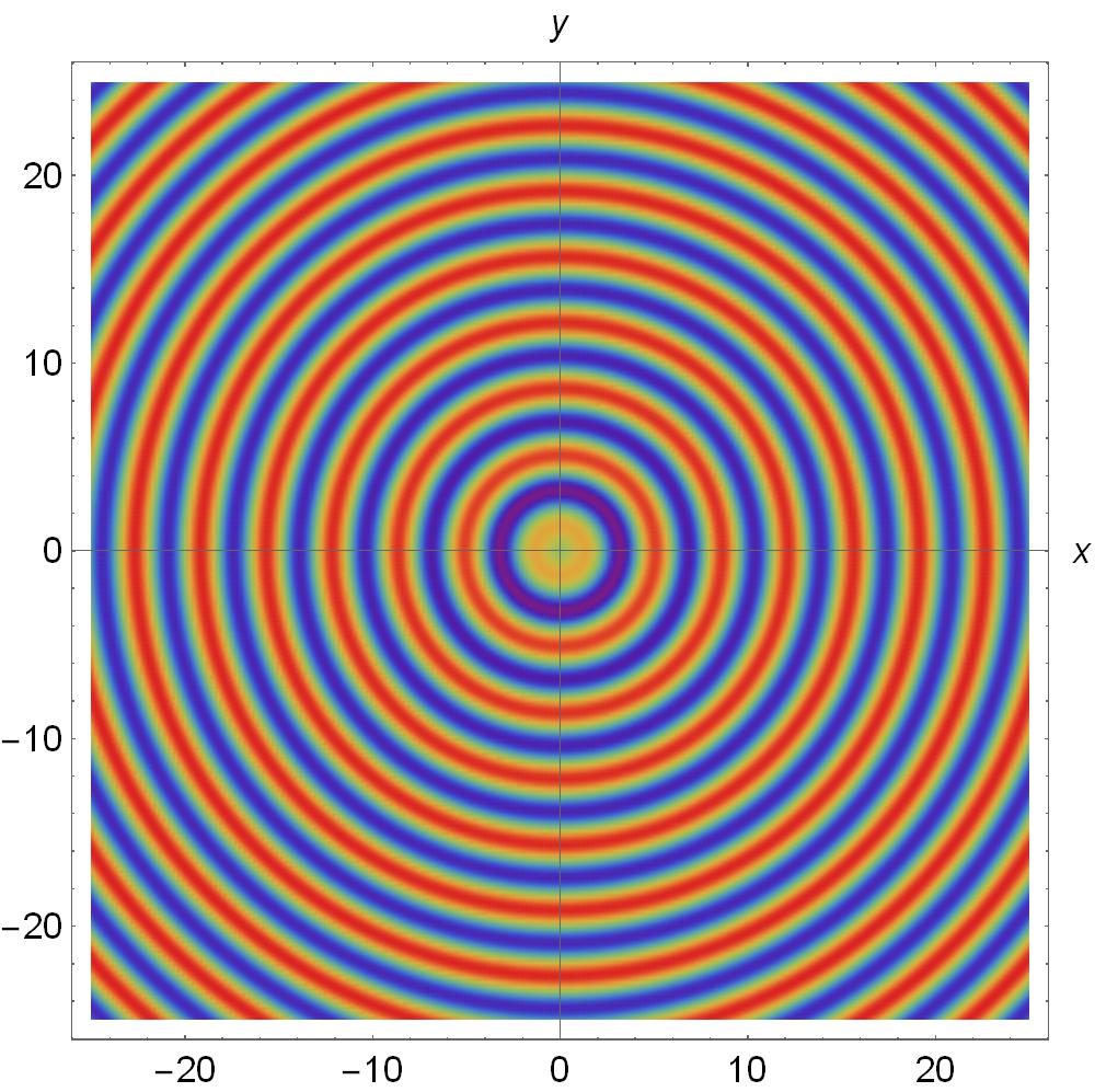
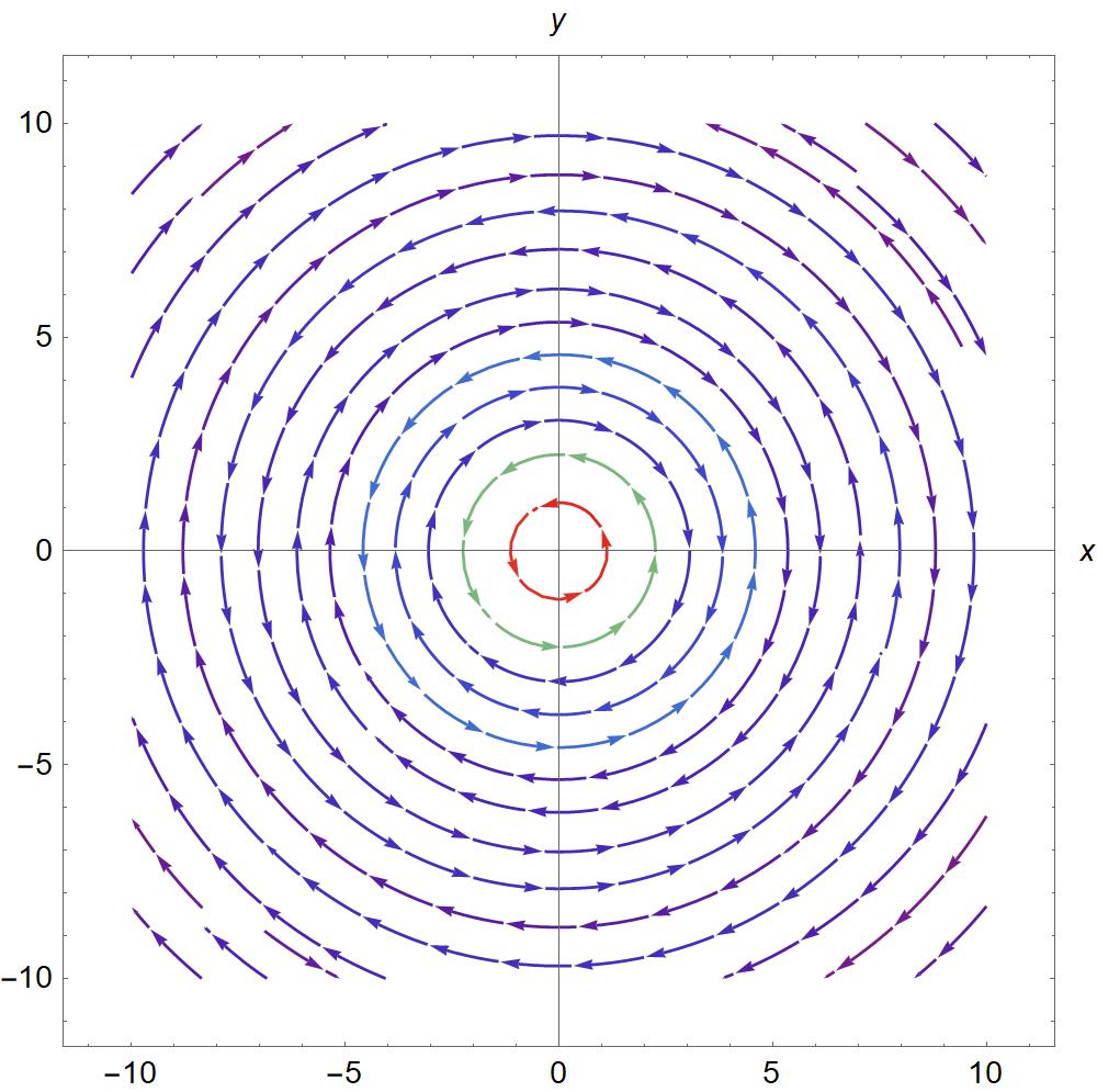
Fig. (3) shows the transverse amplitude vector with the mixed orbital angular momentum modes given by the equation (34), for different values of , with .
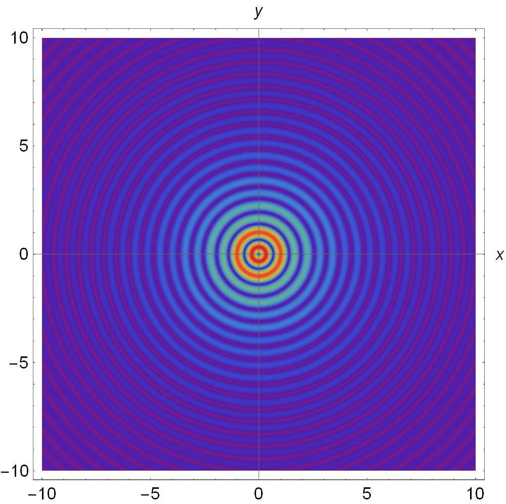
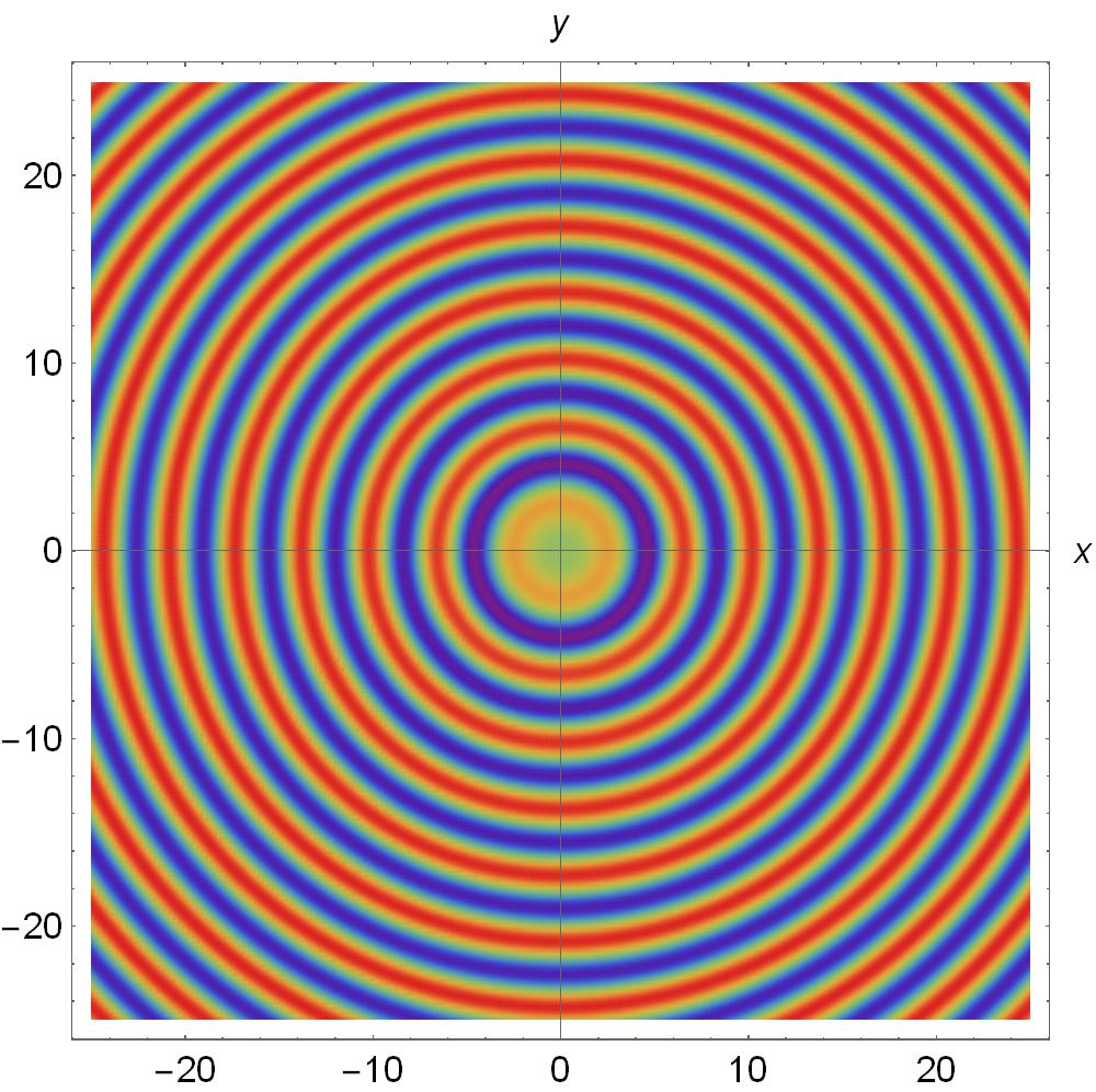
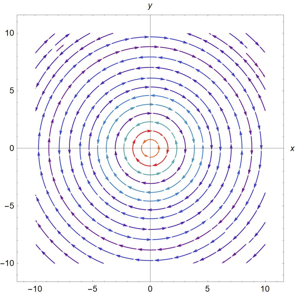
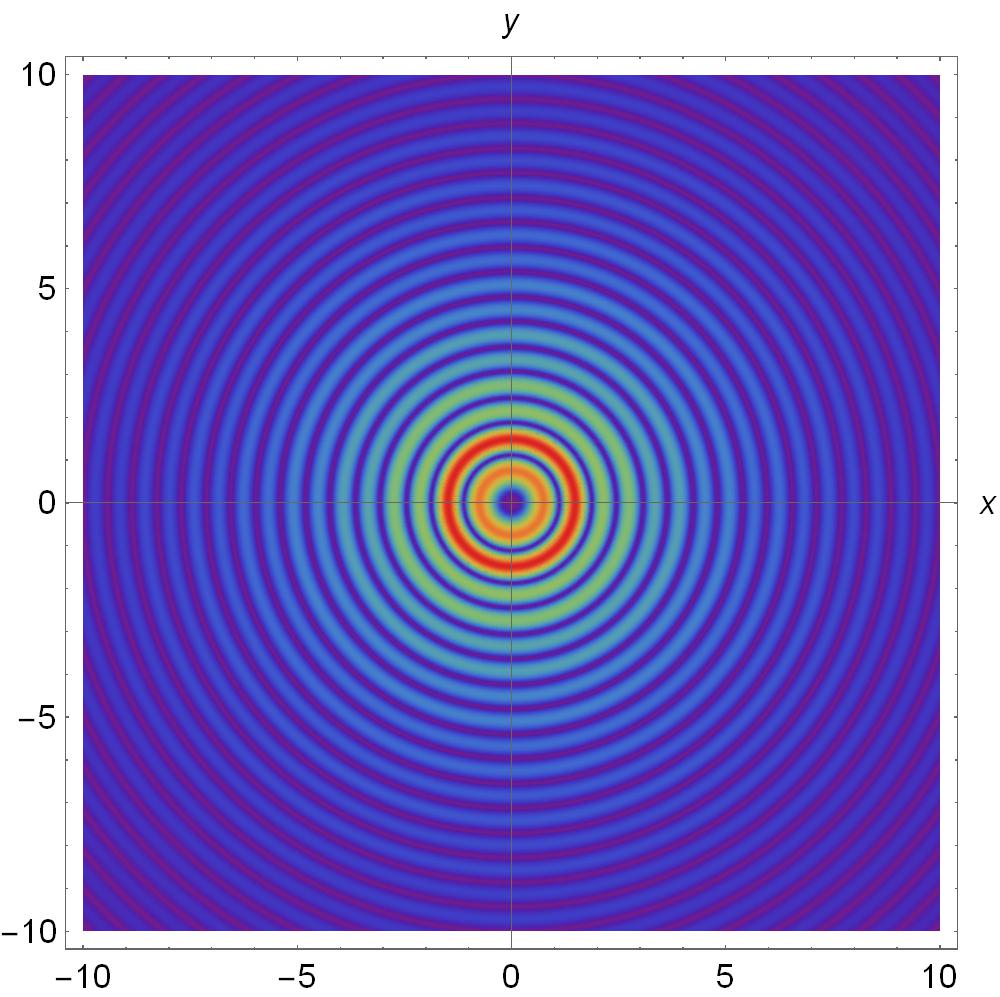
In Fig. (4), we change the azimuthal order to and the polarization is . In both cases the intensity exhibits an azimuthally asymmetric shape which becomes circularly symmetrical.
Lastly, equation (34) can be written using the following Bessel function identity [56], to obtain
| (35) |
It is possible to identify the input field intensity as , and using , we get
| (36) |
Thus, the transversal mixed modes orbital angular momentum can be calculated as the radial derivative of the input field intensity with a well define topological charge. Notice also that this expression contains the optical parameter, and it is proportional to the topological charge . It is worth mentioning that a similar term was reported theoretically in [57] and tested experimentally in [58], to explain the mechanical action of the spin part of the internal energy flow. There, the authors also showed the possibility of controllable motion of suspended particles by changing the polarization of the input field.
5 Conclusions
We have investigated the transversal and longitudinal propagation of orbital angular momentum for invariant beams using a single scalar potential. We have proved that the invariant beams satisfy Maxwell equations and possess well-defined orbital angular momentum [25]. We have shown that the superposition of non-paraxial vectorial beams with axial symmetry can provide a well defined orbital angular momentum. These results exhibit how the modes superposition affects the angular momentum flux density and causes reverse propagation in the case of the fractional Bessel beams [48, 49]. In [59], the authors have studied the importance to handle the amplitude, phase and polarization in order to design structured fields to study the spin-orbit interactions in Bessel beams. Adopting the single scalar potential approach, presented here, may be useful to find interesting applications, as the electromagnetic spin and canonical momentum for paraxial and nonparaxial beams recently reported in [60, 61, 62].
References
- [1] L. Allen, M. W. Beijersbergen, R. J. C. Spreeuw, and J. P. Woerdman, Orbital angular momentum of light and the transformation of Laguerre-Gaussian laser modes Phys. Rev. A 45,11, 8185–1889 (1992).
- [2] Alison M. Yao and Miles J. Padgett, Orbital angular momentum: origins, behaviour and applications, Adv. Opt. Photon. 3, 161–204 (2011).
- [3] Miles J. Padgett, Orbital angular momentum 25 years on, Opt. Express 25, 11265–11274 (2017).
- [4] Richard M. Kerber et al. Reading the Orbital Angular Momentum of Light Using Plasmonic Nanoantennas, ACS Photonics 4, 4, 891–896 (2017).
- [5] A.E. Willner . et al, Optical communications using orbital angular momentum beams, Adv. Opt. Photon, 7, 1, 66–106 (2015).
- [6] K. Volke-Sepulveda and E. Ley-Koo , General construction and connections of vector propagation invariant optical fields: TE and TM modes and polarization states, J. Opt. A: Pure Appl. Opt., 8, 10, 867–-877 (2006).
- [7] K. Volke-Sepulveda, S. Garces-Chavez, S. Chávez-Cerda, J. Arlt and K. Dholakia , Orbital angular momentum of a high-order Bessel light beam, J. Opt. B: Quantum Semiclass. Opt. 4, S82–S89 (2002).
- [8] Flores-Pérez A., Hernández J., Jáuregui R. and Volke-Sepúlveda K., Experimental generation and analysis of first-order TE and TM Bessel modes in free space, Opt. Lett 31, 11, 1732–1734 (2006).
- [9] P.L Marston, Scattering of a Bessel beam by a sphere, J. Acoust. Soc. Am. 121, 2, 753–758, (2007). P.L. Marston ,Scattering of a Bessel beam by a sphere II: Helicoidal case shell example, J. Acoust. Soc. Am. 124, 5, 2905–2910 (2008). A. Belafhal, A. Chafiq, and Z. Hricha, Scattering of Mathieu beams by a rigid sphere. Opt. Comm. 284, 3030–3035 (2011). A. Belafhal, L. Ez-Zariy, A. Chafiq and Z. Hricha, Analysis of the scattering far field of a nondiffracting parabolic beam by a rigid sphere. Phys. and Chem. News, 60, 15–21 (2011).
- [10] Hamed Shoorian, Scattering of linearly polarized Bessel beams by dielectric spheres, Journal of Quantitative Spectroscopy & Radiative Transfer 199, 12–19 (2017).
- [11] I. Rondón Ojeda, Francisco Soto Eguibar, Generalized optical theorem for propagation invariant beams, Optik 137, 17–24 (2017).
- [12] M. Rajabi and A, Mojahed, Acoustic radiation force control: Pulsating spherical carriers, Ultrasonics 83, 146–156 (2018).
- [13] H.E. Hernández-Figueroa, M. Zamboni-Rached. and E. Recami , Non-diffracting Waves, John Wiley & Sons, (2013).
- [14] J. Durnin, Exact solutions for nondiffracting beams. I. The scalar theory, J.Soc. Am A 4, 651–654 (1987).
- [15] J.C. Gutiérrez-Vega, M.D. Iturbe-Castillo and S. Chávez-Cerda, Alternative formulation for invariant optical fields: Mathieu beams, Opt. Lett 25, 20, 1493–1495 (2000).
- [16] Miguel A. Bandres, Julio C. Gutiérrez-Vega, and Sabino Chávez-Cerda, Parabolic nondiffracting optical wave fields, Op. Lett 29, 44–46 (2004).
- [17] E.T. Whitaker, On the partial differential equations of mathematical physics, Math. Ann. 57, 333–355 (1902).
- [18] M. Nieto Vesperinas, Scattering and Diffraction in Physical Optics, Wiley, New York (1991).
- [19] Z. Bouchal, Nondiffracting optical beams: Physical properties, experiments, and applications, Czechoslovak Journal of Physics, 53, 537–578 (2003).
- [20] Florian O. Fahrbach and Alexander Rohrbach, Propagation stability of self-reconstructing Bessel beams enables contrast-enhanced imaging in thick media, Nature Comm. 3, 632 (2012).
- [21] Omar E. Olarte, Jordi Andilla, Emilio J. Gualda, and Pablo Loza-Alvarez, Light-sheet microscopy: a tutorial, Adv. Opt. Photon. 10, 111–179 (2018).
- [22] Daniel Asoubar, Site Zhang, Frank Wyrowski, Michael Kuhn, Parabasal field decomposition and its application to nonparaxial propagation, Opt. Exp. 20, 21, 23502-23517 (2012).
- [23] S. Zhang, C. Hellmann, F. Wyrowski, Algorithm for the propagation of electromagnetic fields through etalons and crystals, App. Physics 56, 15, 4566–4576 (2017).
- [24] A. Novitsky, W. Ding, M. Wang, D. Gao, A. V. Lavrinenko and C.W. Qiu, Pulling cylindrical particles using a soft-nonparaxial tractor beam, Scientific Reports, 7, 652 (2017).
- [25] P. Brandao , Nonparaxial TE and TM vector beams with well-defined orbital angular momentum, Opt. Lett. , 37, 909–911 (2012).
- [26] Irving Rondon-Ojeda and F. Soto-Eguibar, Electromagnetic field theory for invariant beams using scalar potentials, Progress in Electromagnetic Research B, 66, 49–61 (2016).
- [27] A.V. Novitsky, and D. V. Novitsky, Negative propagation of vector Bessel beams, J. Soc. Am. A 24, 2844–2849 (2007).
- [28] Jun Chen, Jack Ng, Z. Lin and C. T. Chan, Optical pulling force, Nature Photonics, 5, 531–534 (2011).
- [29] J. T. Costa, M. G. Silveirinha, and A. Alú, Poynting vector negative-index metamaterials, Phys. Rev. B 83, 165120 (2011).
- [30] A. Novitsky, C. W. Qiu and H. Wang, Single Gradientless Light Beam Drags Particles as Tractor Beams, Phys. Rev. Lett. 107, 203601 (2011).
- [31] Chen Wei Qiu, et al, Engineering light-matter interaction for emerging optical manipulation applications, Nanophotonics 3, 181–201 (2014).
- [32] M. A. Salem and H. Bagci, Energy flow characteristics of vector X-Waves, Opt. Exp. 19, 8526–8532 (2011).
- [33] S. Sukhov and A. Dogariu, On the concept of tractor beams, Op. Lett. 35, 3847–3849 (2010).
- [34] Irving Rondon-Ojeda, Francisco Soto-Eguibar, Properties of the Poynting vector for invariant beams :Negative propagation in Weber beams, Wave Motion 78, 176–-184 (2018).
- [35] Jian Chena, Chenhao Wan and Qiwen Zhan, Vectorial optical fields: recent advances and future prospects, Science Bulletin, 63, 54–74 (2018).
- [36] H. Garcia-Gracia, et al. Measurement of orbital angular momentum with an off-axis superposition of vector modes, J. Opt. 16, 045702 (2014).
- [37] Marco Ornigotti, Claudio Conti, and Alexander Szameit, Effect of Orbital Angular Momentum on Nondiffracting Ultrashort Optical Pulses, Phys. Rev. Lett. 115, 100401 (2015).
- [38] A. Y. Bekshaev, K. Y. Bliokh, and F. Nori, Transverse Spin and Momentum in Two-Wave Interference, Phys. Rev. X, 5, 011039 (2015).
- [39] Manman Li et al. Spinning of particles in optical double-vortex beams, J. Opt. 20, 025401 (2018).
- [40] Igor A. Litvin, Angela Dudley, and Andrew Forbes, Poynting vector and orbital angular momentum density of superpositions of Bessel beams, Opt. Express. 19, 16760–16771 (2011).
- [41] Liang Fang and Jian Wang, Optical angular momentum derivation and evolution from vector field superposition, Opt. Express 25, 23364–23375 (2017).
- [42] J.A. Stratton, Electromagnetic Theory, McGraw-Hill (1941).
- [43] C. P. Boyer, E. G. Kalnins, and W. Miller, Jr.,Symmetry and separation of variables for the Helmholtz and Laplace equations, Nagoya Math. J. 60, 35–80, (1976).
- [44] J.D. Jackson, Classic Electrodynamics, Third Edition, Wiley (1999).
- [45] J. Bajer and R. Horak, Nondiffractive fields, Phys. Rev. E 54, 3, 3052–3054 (1996).
- [46] G. Mendez, A. Fernandez-Vazquez and R. Paez Lopez, Orbital angular momentum and highly efficient holographic generation of nondiffractive TE and TM vector beams, Opt. Comm. 334, 174 –183 (2015).
- [47] D. McGloin, V. Garcés-Chávez, and K. Dholakia, Interfering Bessel beams for optical micromanipulation, Opt. Lett. 28, 657–659 (2003).
- [48] F. G. Mitri, Superposition of nonparaxial vectorial complex-source spherically focused beams: Axial Poynting singularity and reverse propagation, Phys. Rev. A 94, 023801 (2016).
- [49] F. G. Mitri, Reverse propagation and negative angular momentum density flux of an optical nondiffracting nonparaxial fractional Bessel vortex beam of progressive waves, J. Opt. Soc. Am. A 33, 1661–1667 (2016).
- [50] Peter W. Milonni and Robert W. Boyd, Momentum of Light in a Dielectric Medium, Adv. Opt. Photon. 2, 519–553 (2010).
- [51] M. Mazilu, D. J. Stevenson, F. Gunn-Moore, K. Dholakia, Light beats the spread: non-diffracting beams, Laser & Photonics Reviews, 4, 529–547 (2010).
- [52] Chenglong Zhao, Practical guide to the realization of a convertible optical trapping system, Opt. Express 25, 2496–2510 (2017).
- [53] Marco Ornigotti and Andrea Aiello, Radially and azimuthally polarized nonparaxial Bessel beams made simple, Opt. Express 21, 15530–15537 (2013).
- [54] V. V. Kotlyar and A. A. Kovalev, Hermite–Gaussian modal laser beams with orbital angular momentum, J. Soc. Am A 31, 274–282 (2014).
- [55] Yi Wang, Yujie Chen, Yanfeng Zhang, Hui Chen and Siyuan Yu, Generalised Hermite–Gaussian beams and mode transformations, Journal of Optics, 18, 055001 (2016).
- [56] Milton Abramowitz, Handbook of Mathematical Functions, Dover Publications, Inc. New York (1974).
- [57] O. V. Angelsky, et al. , Orbital rotation without orbital angular momentum: mechanical action of the spin part of the internal energy flow in light beams, Opt. Express 20, 3563–3571 (2012).
- [58] O. V. Angelsky, et al, Circular motion of particles suspended in a Gaussian beam with circular polarization validates the spin part of the internal energy flow, Opt. Express 20, 11351–11356 (2012).
- [59] Artur Aleksanyan and Etienne Brasselet, Spin–orbit photonic interaction engineering of Bessel beams, Optica 3, 167–174 (2016).
- [60] KY Bliokh, F Nori, Transverse and longitudinal angular momenta of light, Physics Reports 592, 1–38 (2015).
- [61] K Y Bliokh, M. A Alonso, E A Ostrovskaya and A. Aiello Angular momentum and spin–orbit interaction of nonparaxial light in free space Phys. Rev. A 82 063825 (2010).
- [62] K.Y. Bliokh et al, Theory and applications of free-electron vortex states, Physics Reports, 690 1–70, (2017).