Optomechanical second-order sidebands and group delays in a spinning resonator with parametric amplifier and non-Markovian effects

In recent years, quantities of attention have been paid to the field of optomechanics Aspelmeyer861391 ; Aspelmeyer6529 ; Kippenberg3211172 ; Marquardt240 ; Sainadh92033824 , in which different considerable phenomena have been met. There are different applications such as cooling of a mechanical resonator Metzger4321002 ; Gigan44467 ; Arcizet44471 ; Schliesser5509 ; Meystre525215 , gravitational wave detection Caves4575 ; Abramovici256325 ; Braginsky293228 , optical bistability Nejad562816 ; Sarma331335 ; Shahidani311087 , optomechanical mass sensors Jiang2213773 , quantum measurement Thompson45272 , and detection of weak microwave signals Bagci50781 ; Andrews10321 ; Nejad97053839 in merged quantum mechanical systems with nano and micro mechanics. The recent advance in connection with the present study closely is optomechanically induced transparency (OMIT) Weis3301520 ; Safavi47269 ; Jia91043843 ; Jing59663 ; Wang90023817 . In OMIT, the intense red-detuned optical control field produces anti-Stokes scattering, which alters the optical response of the optomechanical cavity, making it transparent in a narrow bandwidth around the cavity resonance for a probe beam Karuza88013804 . As an analog of electromagnetically induced transparency Fleischhauer77633 ; Agarwal81041803 , OMIT plays an essential role in optical storage and optical telecommunication Chang13023003 ; Fiore107133601 ; Zhou9179 ; Hill31196 . In the last several years, the main progress has concentrated on the linearization of the optomechanical interaction, where we properly explain OMIT by linearizing the optomechanical interaction in the case of ignoring the intrinsic nonlinear nature of the optomechanical coupling Agarwal81041803 ; Huang83043826 . In recent years, nonlinear optical interactions in materials can increase the photons circulating in microcavities, such as parametric amplification and optical Kerr effect Xiong58050302 ; Bartolo94033841 ; Zhou421289 ; Ilchenko92043903 , which has emerged as an important new frontier in cavity optomechanics. In the classical mechanism, nonlinear optomechanical interaction brings about unconventional photon blockade Rabl107063601 ; Flayac96053810 ; Lemonde90063824 , optomechanical chaos Marino87052906 , and sideband generation Xiong86013815 .

Nonreciprocal transmission plays a very important role in the process of quantum information Bi5758 ; Aleahmad72129 ; AbdelMalek528560 ; Bernier8604 due to the characteristics of unidirectional transmission. The nonreciprocal transmission of the optical signal allows the flow of light from one side but blocks it from the other, which resembles the traditional semiconductor p-n junction. Recently, OMIT has been demonstrated in a rotating optomechanical system with a whispering-gallery-mode (WGM) microresonator Schliesser10095015 ; H5367 ; Jiang3371 . The experiment Maayani558569 shows that optical nonreciprocal devices can be achieved by spinning an optomechanical resonator. In such a spinning resonator, due to the Sagnac effect, the frequencies of the clockwise and counterclockwise modes experience Sagnac-Fizeau shifts. Additionally, it also suggests a new scheme to achieve optical nonreciprocity that the optical sidebands strongly rely on the rotary direction of the resonator, which is different from the nonlinearity-based schemes demonstrated Shen10657 ; Ruesink713662 ; Fang7465 ; Cao118033901 ; Li102033526 . The spinning resonator systems have developed rapidly, including nanoparticles sensing Jing51424 , mass sensing Chen14082005 , nonreciprocal photon blockades Huang121153601 ; Li7630 , nonreciprocal phonon lasers Jiang10064037 , unidirectional signal amplification Peng5332000405 , breaking anti-PT symmetry Zhang207594 , and optical solitons Li103053522 .

It has been shown that combining nonlinear optics and optomechanics has resulted in many kinds of physical phenomena to enhance quantum effects Otey93033835 ; Coillet9828 . An optical parametric amplifier (OPA) inside the optomechanical cavity, which is pumped by an external laser, can directly lead to optical amplification and modulate the optomechanical coupling in a way analogous to periodic cavity driving Adamyan92053818 ; Hu100043824 ; Lu114093602 . The OPA is able to generate pairs of down-converted photons, which shows nearly perfect single or dual squeezing. Therefore, the OPA can modify the dynamical instabilities and nonlinear dynamics of the system Mi67115 ; Hu7124 ; Xuereb86013809 . Numerous applications have been studied owing to these features, such as the realization of strong mechanical squeezing Agarwal93043844 , enhancing optomechanical cooling Huang79013821 , the normal-mode splitting Huang80033807 , controlling the photon blockade Sarma96053827 ; Shen98023856 ; Shen101013826 , and the increase of atom-cavity coupling Qin120093601 .

Recently, studying the nonlinear optomechanical interactions in the presence of a coherent mechanical pump has emerged as an important frontier Lemonde111053602 ; Liu111083601 ; Mikkelsen96043832 ; Ferretti85033303 . Due to the existence of nonlinear optomechanical interactions, second-order and higher-order sidebands are generated in optomechanical systems Xiong86013815 ; Kronwald111133601 ; Suzuki92033823 ; Jiao18083034 ; Liu717637 ; Fan65850 . Generation of spectral components at high-order OMIT sidebands is demonstrated analytically, which may have great potential in precise sensing of charges Xiong423630 ; Kong95033820 , phonon number Cohen520522 , weak forces Nunnenkamp111053603 ; Zhao63224211 , single-particle detection Li116 , magnetometer Liu712521 , mass sensor Liu99033822 ; Wang106803908 , and high-order squeezed frequency combs Liu439 . But actually, high-order OMIT sidebands are generally much weaker than the probe signal, which imposes many difficulties in detecting and utilizing the second-order sideband. Therefore, the enhancement and control of second-order sidebands have attracted much interest. Moreover, by controlling the group delay of the output light field, which is caused by rapid phase dispersion, slow light or fast light effects can be achieved Boyd3261074 ; Jiao97013843 ; H5367 ; He351649 ; Li635090 ; Mirza2725515 ; Liao11698 . The fast and slow light effects of the optomechanical system have a wide range of applications in optical communication and interferometry Zimmer92253201 ; Shahriar75053807 . The hybrid nonlinear optomechanical system provides an important platform for further study of the tunable slow and fast effect.

For open systems breuer2002 ; Weiss2008 , only if the coupling between the system and environment is weak, where the characteristic times of the bath are sufficiently smaller than those of the quantum system under study, the Markovian approximation is valid. This means that the Markovian approximation may fail in some cases, e.g., two-state systems, harmonic oscillators, coupled cavities, etc Chang052105 ; Tan032102 ; Longhi063826 ; Leggett5911987 ; breuer1032104012009 ; laine810621152010 ; addis900521032014 ; wibmann860621082012 ; wibmann920421082015 ; shen960338052017 ; lorenzo880201022013 ; rivas1050504032010 ; luo860441012012 ; wolf1011504022008 ; lu820421032010 ; chruscinski1121204042014 ; Zhang063853 ; Zhang19083022 ; Xiong436053 ; Zhao2729082 ; Triana116183602 ; Cheng430385 ; Cheng623678 ; Mu46270 ; Li361363 ; Ding111814 ; Sinha124043603 ; Wu103010601 ; Mu94012334 , where we need to consider the influences of non-Markovian effects on the system dynamics. Moreover, we show that the non-Markovian process proves to be useful in quantum information processing including quantum state engineering, quantum control, quantum channel capacity caruso8612032014 ; darrigo3502112014 ; lofranco900543042014 ; bylicka457202014 ; xue860523042012 , and has been realized in experiment Xiong2019100 ; Cialdi2019100 ; Tang201297 ; Groblacher20156 ; Liu20117 ; Hoeppe2012108 ; Xu201082 ; Madsen2011106 ; Guo2021126 ; Khurana201999 ; Uriri2020101 ; Liu2020102 ; Anderson199347 ; Li2022129 ; breuer880210022016 ; Vega015001 .

The above two considerations motivate us to explore that how to enhance and control the second-order OMIT sidebands and group delays in a spinning resonator with parametric amplifier and non-Markovian effects.

In this paper, we consider the influence of the OPA driven with different pumping frequencies on the second-order sideband generation in a rotating optomechanical system, which is coherently driven by a control field and a probe field. The results show that the second-order sidebands in the rotating resonator can be greatly enhanced in the presence of the OPA and meanwhile, remain the nonreciprocal behavior due to the optical Sagnac effect. The second-order sidebands can be adjusted simultaneously by the pumping frequency and phase of the field driving the OPA, the gain coefficient of the OPA, the rotation speed of the resonator, and the incident direction of the input fields. We compare the differences in efficiency of the second-order sideband generation when the OPA is driven by different pumping frequencies. Due to the Sagnac transformation and presence of the OPA, we find that the group delay of the second-order upper sideband can be tuned by adjusting the nonlinear gain and phase of the field driving the OPA, the rotation speed of the resonator, and the incident direction of the input fields in the spinning optomechanical system. The second-order OMIT sidebands in the spinning resonator are then generalized to the non-Markovian regimes and compared with the Markovian approximation in the wideband limit. The influences of the decay from the non-Markovian environment coupling to an external reservoir on the efficiency of second-order upper sidebands are also investigated. Our paper indicates the advantage of using a hybrid nonlinear system, which provides an effective way to further control and enhance second-order and higher-order sidebands in a nonreciprocal optical device.

The rest of this paper is organized as follows. In Sec. II, we give the efficiency of the second-order sideband and its group delay by solving the Heisenberg-Langevin equations. In Sec. III, we discuss the influence of the OPA excited by a pump driving with the frequency being the sum of the frequencies of the strong control field and the weak probe field driving the resonator on the second-order upper and lower sidebands generation in the spinning resonator. In Sec. IV, we study the group delay of the second-order upper sideband. In Sec. V, we show the influence of the OPA on the second-order sideband generation when the OPA is excited by a pump driving with the frequency setting to twice the frequency of the strong control field. In Sec. VI, we extend nonreciprocal second-order sidebands in the spinning resonator to a non-Markovian bath and compare it with that in the Markovian regime. Moreover, we also study the influences of the decay from the non-Markovian environment coupling to an external reservoir on the efficiency of second-order upper sidebands. Sec. VII is devoted to conclusions.

As schematically shown in Fig. 1(a) and (b), the model we consider is a rotating whispering-gallery-mode (WGM) microresonator (containing an optical parametric amplifier), which is coupled to a stationary tapered fiber. The resonator (driven by a strong control field at frequency ${\omega_{l}}$ and a weak probe field at frequency ${\omega_{p}}$), with optical resonance frequency ${{\omega_{0}}}$ and intrinsic loss ${\kappa_{a}}={{{\omega_{0}}}\mathord{\left/{\vphantom{{{\omega_{0}}}Q}}\right.\kern-1.2pt}Q}$ ($Q$ is the optical quality factor), supports a mechanical breathing mode (frequency ${{\omega_{m}}}$ and effective mass $m$). A control laser and a probe laser are applied to the system via the evanescent coupling of the optical fiber and resonator, and the field amplitudes are given by ${\varepsilon_{l}}=\sqrt{{P_{l}}/\hbar{\omega_{l}}}$ and ${\varepsilon_{p}}=\sqrt{{P_{p}}/\hbar{\omega_{p}}}$, where ${{P_{l}}}$ and ${{P_{p}}}$ are the control and probe powers, respectively. It is well-known that due to the rotation, optical mode frequency experiences Sagnac-Fizeau shift Maayani558569 ; Post39475 ; Malykin431229 , which transforms

	$\displaystyle{\omega_{0}}\to{\omega_{0}}+{\Delta_{s}},$		(1)
	$\displaystyle{\Delta_{s}}=\frac{{nR\Omega{\omega_{0}}}}{c}\left({1-\frac{1}{{{n^{2}}}}-\frac{\lambda}{n}\frac{{dn}}{{d\lambda}}}\right),$		(2)

where $\Omega=\dot{\phi}$ is the angular velocity of the spinning resonator. $n$ and $R$ are the refractive index and radius of the resonator, respectively. $c$ and $\lambda$ are the speed of light and the light wavelength in a vacuum, respectively. The dispersion term ${{dn}\mathord{\left/{\vphantom{{dn}{d\lambda}}}\right.\kern-1.2pt}{d\lambda}}$ represents a negligibly small relativistic (dispersion) correction in the Sagnac-Fizeau shift Maayani558569 ; Jiang10064037 . In Eq. (2), the first term in the parenthesis shows the Sagnac contribution which arises from the rotation of the resonators, while the two last terms with negative signs take into account the Fizeau drag due to the light propagation through a moving resonator medium. As shown in Refs.Agarwal93043844 ; Huang95023844 ; Scully , the operating mechanism of the OPA is standard two-photon squeezing. Embedding the OPA in an optomechanical cavity makes the squeezed state transfer between a photon of a cavity field and a phonon of mechanical mode, which can amplify nonlinear optical responses of the system and reduce mechanical thermal noise and photon shot noise. The Hamiltonian formulation of the system reads

$$\hat{H}={{\hat{H}}_{mech}}+{{\hat{H}}_{opt}}+{{\hat{H}}_{OPA}}+{{\hat{H}}_{drive}},$$

(3)

with

	$\displaystyle{{\hat{H}}_{mech}}=$	$\displaystyle\frac{{{{\hat{p}}^{2}}}}{{2m}}+\frac{1}{2}m\omega_{m}^{2}{{\hat{x}}^{2}}+\frac{{\hat{p}_{\phi}^{2}}}{{2m{{\left({R+\hat{x}}\right)}^{2}}}},$		(4)
	$\displaystyle{{\hat{H}}_{opt}}=$	$\displaystyle\hbar\left({{\omega_{0}}+{\Delta_{s}}}\right){{\hat{a}}^{\dagger}}\hat{a}-\hbar\xi{{\hat{a}}^{\dagger}}\hat{a}\hat{x},$
	$\displaystyle{\hat{H}_{OPA}}=$	$\displaystyle i\hbar G({\hat{a}^{{\dagger}2}}{e^{i\theta}}{e^{-i{\omega_{g}}t}}-H.c.),$
	$\displaystyle{{\hat{H}}_{drive}}=$	$\displaystyle i\hbar\sqrt{{\kappa_{ex}}}\left({{\varepsilon_{l}}{{\hat{a}}^{\dagger}}{e^{-i{\omega_{l}}t}}+{\varepsilon_{p}}{{\hat{a}}^{\dagger}}{e^{-i{\omega_{p}}t}}-H.c.}\right),$

where ${\hat{p}}$, ${\hat{x}}$, ${\hat{\phi}}$, ${{\hat{p}}_{\phi}}$ describe the momentum, position, rotation angle, and angular momentum operators, with commutation relations $[{\hat{x},{\kern 1.0pt}\hat{p}}]=[{\hat{\phi},{\kern 1.0pt}{{\hat{p}}_{\phi}}}]=i\hbar$ Davuluri11264002 . H.c. stands for the Hermitian conjugate. $\hat{a}\left({{{\hat{a}}^{\dagger}}}\right)$ is the annihilation (creation) operator of the cavity field with resonance frequency ${{\omega_{0}}}$. $\xi={{{\omega_{0}}}\mathord{\left/{\vphantom{{{\omega_{0}}}R}}\right.\kern-1.2pt}R}$ is the optomechanical coupling. ${{\hat{H}}_{OPA}}$ describes the coupling of the intracavity field with the OPA (pump frequency $\omega_{g}$). $G$ is the nonlinear gain of the OPA, which is proportional to the pump power driving amplitude. $\theta$ is the phase of the field driving the OPA Shahidani88053813 . We assume that this OPA with a second-order nonlinearity crystal is excited by a pump driving with the frequency $\omega_{g}={{\omega_{l}}+{\omega_{p}}}$ Liu99033822 in Fig. 1(c), so that the signal light and idler light in OPA have the same frequency $({\omega_{l}}+{\omega_{p}})/2$ Nation841 ; Leghtas347853 ; Adiyatullin81329 ; Clerk821155 . ${{\hat{H}}_{drive}}$ describes the interaction of the cavity field with the control field and that of the cavity field with the probe field, where ${{\kappa_{ex}}}$ is the loss caused by the resonator-fiber coupling.

In the rotating frame at the control frequency ${{\omega_{l}}}$, the Hamiltonian (3) becomes

	$\displaystyle{{\hat{H}}_{eff}}=$	$\displaystyle\hbar\left({{\Delta_{0}}-\xi\hat{x}+{\Delta_{s}}}\right){{\hat{a}}^{\dagger}}\hat{a}+\frac{{{{\hat{p}}^{2}}}}{{2m}}+\frac{1}{2}m\omega_{m}^{2}{{\hat{x}}^{2}}$		(5)
		$\displaystyle+\frac{{\hat{p}_{\phi}^{2}}}{{2m{{\left({R+\hat{x}}\right)}^{2}}}}+i\hbar G({\hat{a}^{{\dagger}2}}{e^{-i{\Delta_{p}}t}}{e^{i\theta}}-H.c.)$
		$\displaystyle+i\hbar\sqrt{{\kappa_{ex}}}\left[{\left({{\varepsilon_{l}}+{\varepsilon_{p}}{e^{-i{\Delta_{p}}t}}}\right){{\hat{a}}^{\dagger}}-H.c.}\right],$

where ${\Delta_{0}}={\omega_{0}}-{\omega_{l}}$ and ${\Delta_{p}}={\omega_{p}}-{\omega_{l}}{\kern 1.0pt}$. When the control field is injected at the red-detuned sideband of the cavity resonance ($\Delta_{p}=\omega_{m}$), the transition $\left|{{n_{p}},{n_{m}}+1}\right\rangle\leftrightarrow\left|{{n_{p}}+1,{n_{m}}}\right\rangle$ occurs. Moreover, $\left|{{n_{p}},{n_{m}}}\right\rangle$ couples with $\left|{{n_{p}}+1,{n_{m}}}\right\rangle$ through the probe field which is in resonance with the cavity mode ($\omega_{p}=\omega_{0}$). In this case, the destructive interference of these two excitation pathways occurs, which leads to OMIT Weis3301520 in Fig. 1(c) with pump frequency $\omega_{g}=\omega_{l}+\omega_{p}$ (see Sec. II-IV, Sec. VI) and Fig. 1(d) with pump frequency $\omega_{g}=2\omega_{l}$ (see Sec. V), where OPA has almost no influence on the interference paths. With the operator expectation values defined by $a\equiv\langle{\hat{a}}\rangle$ , $x\equiv\langle{\hat{x}}\rangle$ , $\phi\equiv\langle{\hat{\phi}}\rangle$, and ${p_{\phi}}\equiv\langle{{{\hat{p}}_{\phi}}}\rangle$, the Heisenberg-Langevin equations of the spinning optomechanical system can be derived as

	$\displaystyle\dot{a}=-\left[{\kappa+i\left({{\Delta_{0}}-\xi x+{\Delta_{s}}}\right)}\right]a$
	$\displaystyle\qquad+\sqrt{{\kappa_{ex}}}\left({{\varepsilon_{l}}+{\varepsilon_{p}}{e^{-i{\Delta_{p}}t}}}\right)+2G{a^{*}}{e^{i\theta}}{e^{-i{\Delta_{p}}t}},$		(6)
	$\displaystyle m(\ddot{x}+{\Gamma_{m}}\dot{x}+\omega_{m}^{2}x)=\hbar\xi{a^{*}}a+\frac{{p_{\phi}^{2}}}{{m{R^{3}}}},$		(7)
	$\displaystyle\dot{\phi}=\frac{{{p_{\phi}}}}{{m{R^{2}}}},$		(8)
	$\displaystyle{{\dot{p}}_{\phi}}=0,$		(9)

where $\kappa=({\kappa_{a}}+{\kappa_{ex}})/2$ and $\Gamma_{m}$ are the dissipations of the cavity and the damping of the mechanical mode, respectively. The derivation of Eqs. (6)-(9) can be found in Appendix. Focusing on the mean response of the system to the probe field, we write the operators for their expectation values by means of the mean-field approximation and safely ignore the quantum noise terms with strong driving conditions.

In this case, we assume the control field is much stronger than the probe field (${\varepsilon_{l}}\gg{\varepsilon_{p}}$), which induces that we can use the perturbation method to deal with Eqs. (6)-(9). The control field provides a steady-state solution of the system, while the probe field is treated as the perturbation of the steady state. We then follow the standard procedure, which decomposes the expectation value of all operators as a sum of their steady-state value and small fluctuations around the steady-state value Weis3301520 ; Xiong86013815

	$\displaystyle a=$	$\displaystyle{a_{s}}+A_{1}^{+}{e^{-i{\Delta_{p}}t}}+A_{1}^{-}{e^{i{\Delta_{p}}t}}+A_{2}^{+}{e^{-2i{\Delta_{p}}t}}+A_{2}^{-}{e^{2i{\Delta_{p}}t}},$		(10)
	$\displaystyle x=$	$\displaystyle{x_{s}}+X_{1}^{+}{e^{-i{\Delta_{p}}t}}+X_{1}^{-}{e^{i{\Delta_{p}}t}}+X_{2}^{+}{e^{-2i{\Delta_{p}}t}}+X_{2}^{-}{e^{2i{\Delta_{p}}t}},$

in which $A_{2}^{+}$ ($A_{2}^{-}$) is the amplitude of second-order upper (lower) sideband and corresponds to the responses at the original frequencies $2{\omega_{p}}-{\omega_{l}}$ ($3{\omega_{l}}-2{\omega_{p}}$). We are committed to the fundamental OMIT and its second-order sideband process so that the higher-order sidebands in Eq. (10) are ignored. By substituting Eq. (10) into Eqs. (6)-(9) and comparing the coefficients of the same order, the steady-state solutions are obtained as

	$\displaystyle{a_{s}}=$	$\displaystyle\frac{{\sqrt{{\kappa_{ex}}}{\varepsilon_{l}}}}{{\kappa+i\Delta}},$		(11)
	$\displaystyle{x_{s}}=$	$\displaystyle\frac{{\hbar\xi{{\left|{{a_{s}}}\right|}^{2}}}}{{m\omega_{m}^{2}}}+R{\left({\frac{\Omega}{{{\omega_{m}}}}}\right)^{2}},$

where $\Delta{\rm{=}}{\Delta_{0}}-\xi{x_{s}}+{\Delta_{s}}$, and $\Omega{\rm{=}}{{d\phi}\mathord{\left/{\vphantom{{d\theta}{dt}}}\right.\kern-1.2pt}{dt}}$ is the angular velocity of the spinning resonator. It is clear that the revolving speed of the resonator and Sagnac-Fizeau shift ${\Delta_{s}}$ affect the values of both the mechanical displacement ${x_{s}}$ and intracavity photon number ${\left|{{a_{s}}}\right|^{2}}$. Substituting Eq. (10) into Eqs. (6)-(9), we gain six algebra equations, which can be divided into two groups. The first group describes the linear response of the probe field

$$\begin{split}{\sigma_{1}}\left({{\Delta_{p}}}\right)A_{1}^{+}&=i\xi{a_{s}}X_{1}^{+}+2G{e^{i\theta}}a_{s}^{*}+\sqrt{{\kappa_{ex}}}{\varepsilon_{p}},\\ {\sigma_{2}}\left({{\Delta_{p}}}\right)A_{1}^{-*}&=-i\xi a_{s}^{*}X_{1}^{+},\\ \chi\left({{\Delta_{p}}}\right)X_{1}^{+}&=\hbar\xi({a_{s}}A_{1}^{-*}+a_{s}^{*}A_{1}^{+}),\end{split}$$

(12)

while the second group corresponds to the second-order sideband process

$$\begin{split}{\sigma_{1}}(2{\Delta_{p}})A_{2}^{+}&=i\xi({a_{s}}X_{2}^{+}+A_{1}^{+}X_{1}^{+})+2G{e^{i\theta}}A_{1}^{-*},\\ {\sigma_{2}}\left({2{\Delta_{p}}}\right)A_{2}^{-*}&=-i\xi(a_{s}^{*}X_{2}^{+}+A_{1}^{-*}X_{1}^{+}),\\ \chi\left({2{\Delta_{p}}}\right)X_{2}^{+}&=\hbar\xi(a_{s}^{*}A_{2}^{+}+{a_{s}}A_{2}^{-*}+A_{1}^{-*}A_{1}^{+}),\end{split}$$

(13)

with

	$\displaystyle{\sigma_{1}}\left({n{\Delta_{p}}}\right)$	$\displaystyle=$	$\displaystyle\kappa+i\Delta-in{\Delta_{p}},$
	$\displaystyle{\sigma_{2}}\left({n{\Delta_{p}}}\right)$	$\displaystyle=$	$\displaystyle\kappa-i\Delta-in{\Delta_{p}},$
	$\displaystyle\chi\left({n{\Delta_{p}}}\right)$	$\displaystyle=$	$\displaystyle m(\omega_{m}^{2}-i{\Gamma_{m}}n{\Delta_{p}}-\Delta_{p}^{2}).$

Moreover, we can easily get the linear and second-order nonlinear responses of the system

$$\begin{split}A_{1}^{+}&=\frac{{D+{\sigma_{2}}\left({{\Delta_{p}}}\right)\chi\left({{\Delta_{p}}}\right)}}{{{f_{3}}\left({{\Delta_{p}}}\right)}}(\sqrt{{\kappa_{ex}}}{\varepsilon_{p}}+2G{e^{i\theta}}a_{s}^{*}),\\ X_{1}^{+}&=\frac{{\hbar\xi a_{s}^{*}{\sigma_{2}}\left({{\Delta_{p}}}\right)}}{{D+{\sigma_{2}}\left({{\Delta_{p}}}\right)\chi\left({{\Delta_{p}}}\right)}}A_{1}^{+},\\ A_{1}^{-*}&=\frac{{-i\xi a_{s}^{*}}}{{{\sigma_{2}}\left({{\Delta_{p}}}\right)}}X_{1}^{+},\end{split}$$

(14)

and

$$\begin{split}A_{2}^{+}&=\frac{{-D{\xi^{2}}{a_{s}}X_{1}^{+2}+i\xi{f_{1}}A_{1}^{+}X_{1}^{+}-2i\xi G{e^{i\theta}}a_{s}^{*}{f_{2}}X_{1}^{+}}}{{{\sigma_{2}}\left({{\Delta_{p}}}\right){f_{3}}\left({2{\Delta_{p}}}\right)}},\\ X_{2}^{+}&=\frac{{\hbar\xi[{\sigma_{2}}(2{\Delta_{p}})a_{s}^{*}A_{2}^{+}+{\sigma_{2}}(2{\Delta_{p}})A_{1}^{+}A_{1}^{-*}-i\xi{a_{s}}A_{1}^{-*}X_{1}^{+}]}}{{{f_{2}}}},\\ A_{2}^{-}&=\frac{{i\xi}}{{{\sigma_{2}}{{\left({2{\Delta_{p}}}\right)}^{*}}}}({a_{s}}X_{2}^{-}+A_{1}^{-}X_{1}^{-}),\end{split}$$

(15)

where

$$\begin{split}D&=i\hbar{\xi^{2}}{\left|{{a_{s}}}\right|^{2}},\\ {f_{1}}&=iD{\Delta_{p}}+{\sigma_{2}}\left({{\Delta_{p}}}\right){\sigma_{2}}\left({2{\Delta_{p}}}\right)\chi\left({2{\Delta_{p}}}\right),\\ {f_{2}}&=D+{\sigma_{2}}\left({2{\Delta_{p}}}\right)\chi\left({2{\Delta_{p}}}\right),\\ {f_{3}}\left({n{\Delta_{p}}}\right)&=2iD\Delta+{\sigma_{1}}(n{\Delta_{p}}){\sigma_{2}}\left({n{\Delta_{p}}}\right)\chi\left({n{\Delta_{p}}}\right).\end{split}$$

By using the standard input-output relations, i.e.,

$${a_{out}}(t)={a_{in}}(t)-\sqrt{{\kappa_{ex}}}a(t),$$

(16)

we obtain the expectation value of the output field of this system

	$\displaystyle{a_{out}}(t)=$	$\displaystyle{C_{1}}{e^{-i{\omega_{l}}t}}+{C_{2}}{e^{-i{\omega_{p}}t}}-\sqrt{{\kappa_{ex}}}A_{1}^{-}{e^{-i(2{\omega_{l}}-{\omega_{p}})t}}$		(17)
		$\displaystyle-\sqrt{{\kappa_{ex}}}A_{2}^{+}{e^{-i(2{\omega_{p}}-{\omega_{l}})t}}-\sqrt{{\kappa_{ex}}}A_{2}^{-}{e^{-i(3{\omega_{l}}-2{\omega_{p}})t}},$

where ${C_{1}}={\varepsilon_{l}}-\sqrt{{\kappa_{ex}}}a{}_{s}$ and ${C_{2}}={\varepsilon_{p}}-\sqrt{{\kappa_{ex}}}A_{1}^{+}$. The first term of Eq. (17) denotes the output with control frequency ${{\omega_{l}}}$, while the second and third terms describe the anti-Stokes and Stokes fields, respectively. The terms $-\sqrt{{\kappa_{ex}}}A_{2}^{+}{e^{-i(2{\omega_{p}}-{\omega_{l}})t}}$ and $-\sqrt{{\kappa_{ex}}}A_{2}^{-}{e^{-i(3{\omega_{l}}-2{\omega_{p}})t}}$ are concerned in the second-order upper and lower sidebands Xiong86013815 .

Subsequently, we introduce the dimensionless quantity to define the efficiency of the second-order upper and lower sidebands Xiong86013815 ; Teufel471204

	$\displaystyle{\eta_{1}}=\left|{-\frac{{\sqrt{{\kappa_{ex}}}A_{2}^{+}}}{{{\varepsilon_{p}}}}}\right|,$		(18)
	$\displaystyle{\eta_{2}}=\left|{-\frac{{\sqrt{{\kappa_{ex}}}A_{2}^{-}}}{{{\varepsilon_{p}}}}}\right|,$		(19)

where the amplitude of the probe pulse is treated as a basic scale to gauge the amplitudes of the output sidebands ${\eta_{1}}$ and ${\eta_{2}}$. The associated group delay of the second-order upper sideband turns out to be Safavi47269 ; Lu1 ; Lu2

$${\tau_{1}}={\left.{\frac{{d{\kern 1.0pt}\arg\left({-\frac{{\sqrt{{\kappa_{ex}}}A_{2}^{+}}}{{{\varepsilon_{p}}}}}\right)}}{{2d{\Delta_{p}}}}}\right|_{{\Delta_{p}}={\omega_{m}}}}.$$

(20)

A positive group delay (${\tau_{1}}>0$) corresponds to slow light phenomenon, while a negative group delay (${\tau_{1}}<0$) corresponds to fast light phenomenon Safavi47269 ; Milonni .

In our numerical simulations, to demonstrate that the observation of the second-order sidebands in a resonator assisted by OPA is within current experimental reach, we calculate Eqs. (18)-(20) with parameters from Refs.Maayani558569 ; Righini34435 ; Zhang1321 : $\lambda=1550$ nm, $R=0.25$ mm (the resonator radius), $m=25$ ng, $n=1.44$, $Q={\omega_{0}}/\kappa=4.5\times{10^{7}}$, ${\omega_{m}}=100$ MHz, ${\Gamma_{m}}=0.1$ MHz, ${\kappa_{a}}={\kappa_{ex}}={\omega_{0}}/Q$, ${P_{p}}=0.05{P_{l}}$, and ${\Delta_{0}}={\omega_{m}}$, respectively. We rotate the resonator clockwise, where $\Omega>0$ stands for the light coming from the left-hand side and $\Omega<0$ denotes the light coming from the right-hand side.

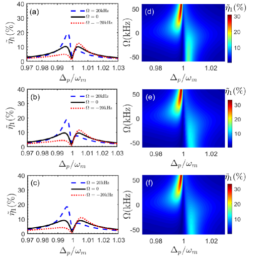
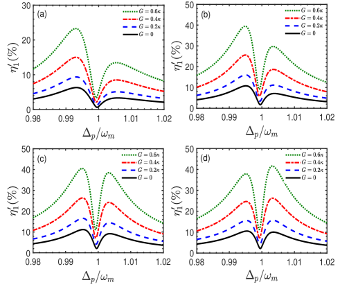
To see the influence of resonator rotation and OPA on the second-order sideband generation, the efficiency of second-order upper sideband generation is investigated as a function of frequency ${\Delta_{p}}/{\omega_{m}}$ shown in Fig. 2. In Fig. 2(a), we discuss that the efficiency ${\eta_{1}}$ of the second-order upper sideband varies with ${\Delta_{p}}$ without the participation of OPA, i.e., the nonlinear gain of the OPA $G=0$, the phase of the field driving the OPA $\theta=0$. Under the resonator stationary, we find two located peaks of second-order sideband spectra and a local minimum near the resonance condition ${\Delta_{p}}={\omega_{m}}$. By spinning the resonator, the peak position of ${\eta_{1}}$ has different moves when the driving fields come from different directions. By adjusting the frequency ${\Delta_{p}}/{\omega_{m}}$, we can get enhanced efficiency of the second-order sideband while driving the resonator from one direction and suppressed efficiency while driving from the opposite direction. For example, within ${\Delta_{p}}/{\omega_{m}}$ in the range from $0.99$ to $1$, ${\eta_{1}}$ is enhanced in the case of $\Omega>0$, while it is suppressed in the case of $\Omega<0$. Obviously, this spinning-induced direction-dependent nonreciprocal behavior can be attributed to the optical Sagnac effect induced by a spinning resonator. As shown in Fig. 2(b), the efficiency ${\eta_{1}}$ gets larger in the presence of OPA. To be more specific, for $G=0.2\kappa,\theta=0$ and $\Omega=20$ kHz, the efficiency ${\eta_{1}}$ can increase from ${\rm{19}}{\rm{.5\%}}$ to $27.2{\rm{\%}}$ at ${\Delta_{p}}=0.997{\omega_{m}}$. When the system is driven from the right, i.e., $\Omega=-20$ kHz, the efficiency ${\eta_{1}}$ also can increase from $12.4{\rm{\%}}$ to $21.6{\rm{\%}}$ at ${\Delta_{p}}=1.004{\omega_{m}}$. Fig. 2(c) shows that the efficiency ${\eta_{1}}$ can also be adjusted by tuning $\theta$. What can be seen clearly is when $\theta$ changes from $\theta=0$ to $\theta=3\pi/2$, in the case of $G=0.2\kappa$ and $\Omega=20$ kHz, the maximum value of ${\eta_{1}}$ increases to $37.4{\rm{\%}}$. In the case of $\Omega=-20$ kHz, the maximum value increases to $29.2{\rm{\%}}$. We see that the efficiency of the second-order upper sideband is sensitive to the variation of the nonlinear gain of the OPA and phase of the field driving the OPA, which indicates the advantage of using a hybrid nonlinear system. According to Eqs. (14)-(15), such phenomena coming from the amplitudes of second-order sidebands $A_{2}^{+}$ and $A_{2}^{-}$ are related directly to the Sagnac-Fizeau shift and OPA. With the purpose of seeing the influence of the OPA on the second-order sideband generation more clearly, the efficiency ${\eta_{1}}$ as a function of both ${\Delta_{p}}$ and $\Omega$ is shown in Fig. 2(d)-(f).

To explore the role of OPA in this resonator, we illustrate the efficiency ${\eta_{1}}$ of the second-order upper sideband versus the probe-pulsed detuning ${\Delta_{p}}$ with different nonlinear gain $G$ of the OPA and phase $\theta$ of the field driving the OPA, when the system is driven from the right-hand side ($\Omega=-20$ kHz) in Fig. 3. We find when the nonlinear gain $G$ of the OPA increases from $0$ to $G=0.6\kappa$, the efficiency ${\eta_{1}}$ can be significantly enhanced in Fig. 3(a). The enhancement effect at the probe-pulsed detuning ${\Delta_{p}}/{\omega_{m}}<1$ is much weaker than at ${\Delta_{p}}/{\omega_{m}}>1$. Fig. 3(c) shows that the second-order sideband behavior of the output field can also be adjusted by tuning $\theta$. In the case of $G=0.2\kappa$, we find that compared with $\theta=0$, both $\theta=\pi/2$ and $\theta=\pi$ result in lower efficiency ${\eta_{1}}$ of the second-order upper sideband, but $\theta=3\pi/2$ leads to enhanced efficiency. In Fig. 3(d), ${\eta_{1}}$ as a function of detuning ${\Delta_{p}}$ and the phase $\theta$ of the OPA is plotted. In the range shown, the maximum value of efficiency ${\eta_{1}}$ is about $30.2\%$ at $\theta=1.6\pi$ and ${\Delta_{p}}=1.004{\omega_{m}}$. Specifically, the efficiency is enhanced when $\theta\in(1.6\pi,{\kern 1.0pt}{\kern 1.0pt}2\pi)$ and suppressed at other values. Besides, as is illustrated in Fig. 3(b) and (d), regardless of what nonlinear gain $G$ and $\theta$ is to increase, the located maximums of the efficiency ${\eta_{1}}$ are still located at the same position of the probe-pulsed detuning. This phenomenon can be explained by Refs.Weis3301520 ; Xiong86013815 , which shows there are some connections between OMIT and the second-order sideband process. When OMIT occurs, the second-order sideband process is subdued. The linewidth of the OMIT window is related to the intracavity photon number

$${\Gamma_{OMIT}}\approx{\Gamma_{\rm{m}}}+\frac{{{\xi^{2}}x_{zpf}^{2}}}{\kappa}{\left|{{a_{s}}}\right|^{2}},$$

(21)

where ${x_{zpf}}=\sqrt{\hbar/2m{\omega_{\rm{m}}}}$. By perturbation theory, we can get the intracavity photon number ${\left|{{a_{s}}}\right|^{2}}$ in Eq. (11), which is independent of other perturbation terms such as probe pulse and nonlinear gain of the OPA. That is to say, the positions of these local maximums of sideband spectra only depend on the intrinsic structural parameters of an optomechanical system and intensity of the control field. As a result, the OPA not only improves the sideband efficiency of the second-order sideband but also keeps the locality of maximum values of the sideband efficiency.

In Fig. 4, we discuss the influence of resonator rotation and OPA on the second-order lower sideband generation. As shown in Fig. 4(a), unlike the second-order upper sideband, the second-order lower sideband has no local minimum but only one peak. The efficiency is much smaller than the second-order upper sideband. In detail, with neither resonator rotation nor the OPA drive, ($G=0$, $\Omega=0$), both peaks of ${\eta_{1}}$ are about $19.6\%$ and the peak of ${\eta_{2}}$ is only $0.82\%$. Furthermore, the second-order lower sideband exhibits non-reciprocal characteristics due to the rotation of the resonator, which is more pronounced at ${\Delta_{p}}/{\omega_{m}}>1$. In detail, compared with the stationary resonator (i.e., no spinning with $\Omega=0$), the spinning resonator increases for $\Omega=-20$ kHz, while it decreases for $\Omega=20$ kHz at ${\Delta_{p}}/{\omega_{m}}>1$ in Fig. 4(a). In Fig. 4(d), we find that for the same resonator speed, the enhancement effect is more pronounced when the device is driven from the right side ($\Omega<0$) than from the left side ($\Omega>0$). For example, for $\Omega=-60$ kHz, the maximum value of ${\eta_{2}}$ is $3.04\%$ at ${\Delta_{p}}/{\omega_{m}}=1.003$. For $\Omega=60$ kHz, the maximum value of ${\eta_{2}}$ is $0.97\%$ at ${\Delta_{p}}/{\omega_{m}}=0.999$. In Fig. 4(b) and (c), as with the second-order upper sideband, the presence of OPA significantly improves the efficiency of the second-order lower sideband, which also keeps the locality of maximum values of the sideband efficiency. In detail, for $\Omega=-20$ kHz, when the nonlinear gain $G$ of OPA increases from 0 to $0.2\kappa$, the maximum value of ${\eta_{2}}$ increases from $1.08\%$ to $1.75\%$ at ${\Delta_{p}}/{\omega_{m}}=1.001$. Besides, when the phase $\theta$ of the OPA increases from 0 to $3\pi/2$, the maximum value of ${\eta_{2}}$ can be increased to $2.51\%$, which is more than twice the value without OPA.

We show that the presence of OPA only causes a change in the peak of ${\eta_{1}}$ and has almost no influence on asymmetry (see black-solid line in Fig. 2(a)-(c) for $\Omega=0$, and black-solid line in Fig. 4(a)-(c) for $\Omega=0$).

Without the OPA ($G=0$), the asymmetric line shape of ${\eta_{1}}$ with regard to ${\Delta_{p}}={\omega_{m}}$ and the ${\eta_{2}}$ peak being not exactly at ${\Delta_{p}}={\omega_{m}}$ come from the spinning of the resonator. In this case, the mean mechanical displacement ${x_{s}}$ in Eq. (11) is made up of two terms: the first term is proportional to the intracavity photon number $|{a_{s}}|^{2}$, which is closely related to the Sagnac-Fizeau shift ${\Delta_{s}}=\frac{{nR\Omega{\omega_{0}}}}{c}({1-\frac{1}{{{n^{2}}}}-\frac{\lambda}{n}\frac{{dn}}{{d\lambda}}})$ in Eq. (2) or, equivalently, very sensitive to the angular velocity $\Omega$ of resonator and incident direction of input fields, thus giving rise to the nonreciprocal behavior. The second term $R{(\Omega/{\omega_{m}})^{2}}$ of ${x_{s}}$ makes the mechanical displacement larger due to the rotation. The existence of these two terms together affects the second-order upper and lower sidebands in Eqs. (18) and (19), which lead to the asymmetry of ${\eta_{1}}$ with regard to ${\Delta_{p}}={\omega_{m}}$ and the ${\eta_{2}}$ peak being not exactly at ${\Delta_{p}}={\omega_{m}}$ shown in Fig. 2 to Fig. 4.

In this case, $R{(\Omega/{\omega_{m}})^{2}}$ of ${x_{s}}$ in Eq. (11) originates from an extra term in the Hamiltonian of our model due to the rotation, i.e., the rotational kinetic energy term $\hat{p}_{\phi}^{2}/[2m{({R+\hat{x}})^{2}}]$ in Eq. (4), which is different from the usual situation in Ref.Xiong86013815 . Since $x/R\ll 1$ ($x=\langle{\hat{x}}\rangle$ denotes the expectation value of $\hat{x}$), the term $\hat{p}_{\phi}^{2}/[2m{({R+\hat{x}})^{2}}]$ is approximately equal to $-\hat{p}_{\phi}^{2}\hat{x}/(m{R^{3}})+\hat{p}_{\phi}^{2}/(2m{R^{2}})$ (neglecting second and higher order small quantities about $x/R$). This means that there is an extra force $-\hat{p}_{\phi}^{2}\hat{x}/(m{R^{3}})$ exerted on the mechanical mode making it deviate from its original equilibrium position.

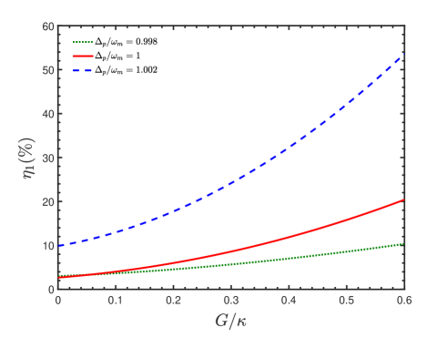
To clearly see the influence of the nonlinear gain $G$ of OPA on the second-order sideband generation, the efficiency ${\eta_{1}}$ is investigated as a function of the nonlinear gain $G$ for different probe-pulsed detuning ${\Delta_{p}}$, as shown in Fig. 5. In detail, when $G$ increases from $0$ to $0.6\kappa$ in the case of ${\Delta_{p}}/{\omega_{m}}=1.002$, the system provides an enhancement of more than five times for the sideband efficiency ${\eta_{1}}$. In general, with the nonlinear gain $G$ increasing, the efficiency ${\eta_{1}}$ of the second-order upper sideband generation increases obviously. The reason is that when the OPA is pumped at $\omega_{g}={\omega_{l}}+{\omega_{p}}$, i.e., twice the frequency of the anti-Stokes field, the parametric frequency conversion between this anti-Stokes field and phonon mode can provide another way to generate an optical second-order sideband, leading to the enhancement of a second-order sideband.

We know the slow light effect is an important result of OMIT, which can be described by the optical group delay Safavi47269 ; He351649 ; Li635090 ; Mirza2725515 ; Liao11698 . It is similar to that of electromagnetically induced transparency, in the region of the narrow transparency window the rapid phase dispersion can cause the group delay given by Eq. (20). A positive group delay (${\tau_{1}}>0$) corresponds to slow light propagation and a negative group delay (${\tau_{1}}<0$) denotes fast light propagation.

In the previous work Safavi47269 ; Milonni , it has been demonstrated that the delay of the transmitted light is only relevant to the pump power in a conventional optomechanical system. In our model, we see clearly from Fig. 6 that the delay time of the second-order upper sideband can be adjusted not only by tuning the speed and direction of rotation of the resonator but also by adjusting the nonlinear gain of the OPA and phase of the field driving the OPA. In Fig. 6(a) and (b), we investigate the group delay of the second-order upper sideband ${\tau_{1}}$ as a function of control laser power ${P_{l}}$ for different $\Omega$. We find that when the resonator is stationary ($\Omega=0$), with the power increasing, ${\tau_{1}}$ tends to advance and even switches into fast light. However, in the presence of resonator rotation, the delay time of the second-order upper sideband will be prolonged at high control powers, which is useful for storage. In detail, as shown in Fig. 6(a), for a resonator speed of $20$ kHz, the group delay time ${\tau_{1}}$ increases when the resonator is driven from the right side ($\Omega=-20$ kHz) and decreases when the resonator is driven from the left side ($\Omega=20$ kHz). The group delay can still reach the conversion from fast light to slow light at this point. Increasing the resonator speed to $40$ kHz, at high control power, when the resonator is driven from the right side ($\Omega=-40$ kHz), the group delay of the second-order sideband is always positive, i.e., slow light is obtained. When the resonator is driven from the left side ($\Omega=40$ kHz), the group delay is always negative and fast light can be obtained. At this point, the switching between fast and slow light disappears. In Fig. 6(b), we show the results of group delay ${\tau_{1}}$ versus control laser power $P_{l}$ in the presence of OPA. In the low power range, the addition of OPA increases the value of ${\tau_{1}}$. More interestingly, at $\Omega=-40$ kHz, the fast and slow light conversion behavior of the group delay disappears, where only slow light effect is obtained.

Now we discuss the influence of the presence of OPA on the delay time of the second-order sideband. In Fig. 6(c) and (d), we display the group delay ${\tau_{1}}$ as a function of the control power ${P_{l}}$ for different parameters of nonlinear gain $G$ and phase $\theta$ of the field driving the OPA, where the resonator is stationary. When the OPA is considered in the optomechanical system, as is expected, the delay time of the second-order upper sideband generation obviously increases with the increasing power. With the nonlinear gain $G$ increasing from $0$ to $0.4\kappa$, the group delay ${\tau_{1}}$ accordingly increases, while the trend of switching between fast and slow light effects remains unchanged. In Fig. 6(d), we see that the ${\tau_{1}}$ is sensitive to the variation of the phase of the OPA. When $\theta=\pi/2$, ${\tau_{1}}$ exhibits a significant transition from fast to slow light, in other words the delay time significantly reduces at low power and increases at high power. Interestingly, for $\theta=3\pi/2$, the valley of the ${\tau_{1}}$ disappears in the low power range, where the group delay exhibits a fast light effect (${\tau_{1}}<0$) in the high power range. Physically, from Eq. (15), when the OPA is added inside the optomechanical coupled system, the quantum interference effect between the probe field and second-order sideband process is related directly to the phase of the OPA, so that the optical-response properties for the probe field become phase-sensitive.

As shown in Fig. 7, the group delay ${\tau_{1}}$ varies with the rotation speed of the resonator $\left|\Omega\right|$ at a fixed control power, where the red sideband ${{\Delta_{p}}={\omega_{m}}}$ is also presented. We find the group delay can achieve the transition from fast to slow light regardless of the direction of incidence of the input fields but with very significant differences. If $\Omega>0$ (the driving fields come from the left-hand side of the fiber), when the rotation speed reaches $101$ kHz, the group delay ${\tau_{1}}$ experiences the conversion from ${\tau_{1}}<0$ to ${\tau_{1}}>0$. However, if $\Omega<0$ (driving from the right-hand side of the fiber), when the rotation speed reaches $30$ kHz, ${\tau_{1}}$ experiences the conversion from ${\tau_{1}}<0$ to ${\tau_{1}}>0$. Therefore, we realize the conversion between the fast light and slow light by controlling the incident direction of the input fields in the spinning system.

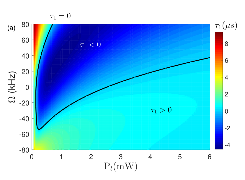
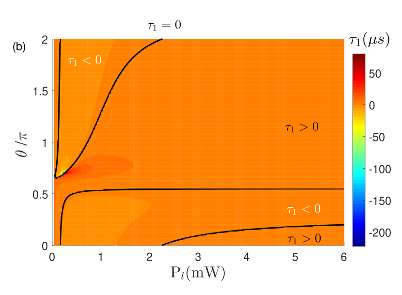
In the above discussion, we see that the group delay of the second-order upper sideband is sensitive to the variation of the rotation speed of the resonator, the direction of incidence of the input fields, and the phase of the field driving the OPA. In Fig. 8(a), the group delay ${\tau_{1}}$ of the second-order upper sideband is plotted as the function of control power ${P_{l}}$ and the rotation speed of the resonator $\Omega$. In Fig. 8(b), ${\tau_{1}}$ is plotted as the function of control power ${P_{l}}$ and the phase $\theta$ of the field driving the OPA. The black curves correspond to ${\tau_{1}}=0$. In this case, we can obtain the slow light effect or fast light effect by properly selecting the values of ${P_{l}}$, $\Omega$, and $\theta$. Moreover, a tunable switch from fast to slow light can be realized by adjusting their values.

The optical degenerate parametric amplifier (OPA), a second-order optical crystal in nature, can generate pairs of down-converted photons and show nearly perfect single or dual squeezing Gerry ; Li100023838 ; Clerk821155 ; Nation841 ; Leghtas347853 ; Shen100023814 . As we all know, placing an OPA pumped by an external laser in the optomechanical cavity can modulate the optomechanical coupling, which can lead to optical amplification directly Adamyan92053818 . We can discuss the influence of different pump frequencies of the driving OPA on the sidebands and compare the amplification of the second-order sidebands in both cases. Now, we vary the frequency of the laser field driving the OPA, so that the OPA is excited by a pump drive with the frequency $\omega_{g}=2{\omega_{l}}$ Li100023838 in Fig. 1(d). The pump photon with frequency $\omega_{g}=2{\omega_{l}}$ is down-converted into an identical pair of photons with frequency ${\omega_{l}}$ after passing through the second-order nonlinearity crystal. ${{\hat{H}}_{OPA}}$ reads

$${\hat{H}_{OPA}}=i\hbar G({\hat{a}^{{\dagger}2}}{e^{i\theta}}{e^{-2i{\omega_{l}}t}}-H.c.).$$

(22)

The total Hamiltonian of the system in the rotating frame at the laser frequency ${{\omega_{l}}}$ is given by

	$\displaystyle{{\hat{H}}_{eff}}=$	$\displaystyle\hbar\left({{\Delta_{0}}-\xi\hat{x}+{\Delta_{s}}}\right){{\hat{a}}^{\dagger}}\hat{a}+\frac{{{{\hat{p}}^{2}}}}{{2m}}+\frac{1}{2}m\omega_{m}^{2}{{\hat{x}}^{2}}$		(23)
		$\displaystyle+\frac{{\hat{p}_{\phi}^{2}}}{{2m{{\left({R+\hat{x}}\right)}^{2}}}}+i\hbar G({\hat{a}^{{\dagger}2}}{e^{i\theta}}-H.c.)$
		$\displaystyle+i\hbar\sqrt{{\kappa_{ex}}}\left[{\left({{\varepsilon_{l}}+{\varepsilon_{p}}{e^{-i{\Delta_{p}}t}}}\right){{\hat{a}}^{\dagger}}-H.c.}\right].$

We can get the equations of motion

	$\displaystyle\dot{a}=-\left[{\kappa+i\left({{\Delta_{0}}-\xi x+{\Delta_{s}}}\right)}\right]a$
	$\displaystyle\qquad+\sqrt{{\kappa_{ex}}}\left({{\varepsilon_{l}}+{\varepsilon_{p}}{e^{-i{\Delta_{p}}t}}}\right)+2G{e^{i\theta}}{a^{*}},$		(24)
	$\displaystyle m(\ddot{x}+{\Gamma_{m}}\dot{x}+\omega_{m}^{2}x)=\hbar\xi{a^{*}}a+\frac{{p_{\phi}^{2}}}{{m{R^{3}}}},$		(25)
	$\displaystyle\dot{\phi}=\frac{{{p_{\phi}}}}{{m{R^{2}}}},$		(26)
	$\displaystyle{{\dot{p}}_{\phi}}=0,$		(27)

where we write the operators for their expectation values by the mean-field approximation. The steady-state solutions of the system are obtained as

$$\begin{split}{\tilde{a}_{s}}&=\frac{{2G{e^{i\theta}}+\kappa-i\tilde{\Delta}}}{{{\kappa^{2}}+{{\tilde{\Delta}}^{2}}-4{G^{2}}}},\\ {{\tilde{x}}_{s}}&=\frac{{\hbar\xi{{\left|{{\tilde{a}_{s}}}\right|}^{2}}}}{{m\omega_{m}^{2}}}+R{\left({\frac{\Omega}{{{\omega_{m}}}}}\right)^{2}},\end{split}$$

(28)

where $\tilde{\Delta}{\rm{=}}{\Delta_{0}}-\xi{{\tilde{x}}_{s}}+{\Delta_{s}}$. It is worth noting that here, unlike Eq. (11), the intracavity photon number ${\left|{{{\tilde{a}}_{s}}}\right|^{2}}$ and displacement of mechanical oscillator ${{\tilde{x}}_{s}}$ strongly depend on the magnitude of nonlinear gain $G$ and phase $\theta$ of the OPA. Eqs. (24)-(27) can be solved analytically with the linearized ansatz

	$\displaystyle a=$	$\displaystyle{\tilde{a}_{s}}+\tilde{A}_{1}^{+}{e^{-i{\Delta_{p}}t}}+\tilde{A}_{1}^{-}{e^{i{\Delta_{p}}t}}+\tilde{A}_{2}^{+}{e^{-2i{\Delta_{p}}t}}+\tilde{A}_{2}^{-}{e^{2i{\Delta_{p}}t}},$
	$\displaystyle x=$	$\displaystyle{{\tilde{x}}_{s}}+\tilde{X}_{1}^{+}{e^{-i{\Delta_{p}}t}}+\tilde{X}_{1}^{-}{e^{i{\Delta_{p}}t}}+\tilde{X}_{2}^{+}{e^{-2i{\Delta_{p}}t}}+\tilde{X}_{2}^{-}{e^{2i{\Delta_{p}}t}}.$

After the ansatz, we obtain six algebra equations, which can be divided into two groups

$$\begin{split}{{\tilde{\sigma}}_{1}}\left({{\Delta_{p}}}\right)\tilde{A}_{1}^{+}&=i\xi{{\tilde{a}}_{s}}\tilde{X}_{1}^{+}+2G{e^{i\theta}}\tilde{A}_{1}^{-*}+\sqrt{{\kappa_{ex}}}{\varepsilon_{p}},\\ {{\tilde{\sigma}}_{2}}\left({{\Delta_{p}}}\right)\tilde{A}_{1}^{-*}&=-i\xi\tilde{a}_{s}^{*}\tilde{X}_{1}^{+}+2G{e^{-i\theta}}\tilde{A}_{1}^{+},\\ \chi\left({{\Delta_{p}}}\right)\tilde{X}_{1}^{+}&=\hbar\xi({{\tilde{a}}_{s}}\tilde{A}_{1}^{-*}+\tilde{a}_{s}^{*}\tilde{A}_{1}^{+}),\end{split}$$

(29)

and

$$\begin{split}{{\tilde{\sigma}}_{1}}\left({2{\Delta_{p}}}\right)\tilde{A}_{2}^{+}&=i\xi({{\tilde{a}}_{s}}\tilde{X}_{2}^{+}+\tilde{A}_{1}^{+}\tilde{X}_{1}^{+})+2G{e^{i\theta}}\tilde{A}_{2}^{-*},\\ {{\tilde{\sigma}}_{2}}\left({2{\Delta_{p}}}\right)\tilde{A}_{2}^{-*}&=-i\xi(\tilde{a}_{s}^{*}\tilde{X}_{2}^{+}+\tilde{A}_{1}^{-*}\tilde{X}_{1}^{+})+2G{e^{-i\theta}}\tilde{A}_{2}^{+},\\ \chi\left({2{\Delta_{p}}}\right)\tilde{X}_{2}^{+}&=\hbar\xi({{\tilde{a}}_{s}}\tilde{A}_{2}^{-*}+\tilde{a}_{s}^{*}\tilde{A}_{2}^{+}+\tilde{A}_{1}^{+}\tilde{A}_{1}^{-*}),\end{split}$$

(30)

with

	$\displaystyle{{\tilde{\sigma}}_{1}}\left({n{\Delta_{p}}}\right)$	$\displaystyle=$	$\displaystyle\kappa+i{\tilde{\Delta}}-in{\Delta_{p}},$
	$\displaystyle{{\tilde{\sigma}}_{2}}\left({n{\Delta_{p}}}\right)$	$\displaystyle=$	$\displaystyle\kappa-i{\tilde{\Delta}}-in{\Delta_{p}},$
	$\displaystyle\chi\left({n{\Delta_{p}}}\right)$	$\displaystyle=$	$\displaystyle m(\omega_{m}^{2}-i{\Gamma_{m}}n{\Delta_{p}}-\Delta_{p}^{2}).$

We get the linear and second-order nonlinear responses of the system

$$\begin{split}\tilde{A}_{1}^{+}&=\frac{{\tilde{D}+{{\tilde{\sigma}}_{2}}({\Delta_{p}})\chi({\Delta_{p}})}}{{{{\tilde{f}}_{4}}({\Delta_{p}})+{{\tilde{f}}_{3}}({\Delta_{p}})}}\sqrt{{\kappa_{ex}}}{\varepsilon_{p}},\\ \tilde{X}_{1}^{+}&=\frac{{\hbar\xi[2G{e^{-i\theta}}{{\tilde{a}}_{s}}+\tilde{a}_{s}^{*}{{\tilde{\sigma}}_{2}}({\Delta_{p}})]}}{{\tilde{D}+{{\tilde{\sigma}}_{2}}({\Delta_{p}})\chi({\Delta_{p}})}}\tilde{A}_{1}^{+},\\ \tilde{A}_{1}^{-*}&=\frac{{-i\xi\tilde{a}_{s}^{*}}}{{{{\tilde{\sigma}}_{2}}({\Delta_{p}})}}\tilde{X}_{1}^{+}+\frac{{2G{e^{-i\theta}}}}{{{{\tilde{\sigma}}_{2}}({\Delta_{p}})}}\tilde{A}_{1}^{+},\end{split}$$

(31)

and

$$\begin{split}\tilde{A}_{2}^{+}&=\frac{{i\hbar{\xi^{2}}{{\tilde{f}}_{6}}\tilde{A}_{1}^{+}\tilde{A}_{1}^{-*}+{{\tilde{f}}_{7}}\tilde{A}_{1}^{-*}\tilde{X}_{1}^{+}+i\xi{{\tilde{f}}_{2}}\tilde{A}_{1}^{+}\tilde{X}_{1}^{+}}}{{{{\tilde{f}}_{4}}\left({2{\Delta_{p}}}\right)+{{\tilde{f}}_{3}}\left({2{\Delta_{p}}}\right)}},\\ \tilde{X}_{2}^{+}&=\frac{{\hbar\xi[{{{\tilde{f}}_{5}}\tilde{A}_{2}^{+}-i\xi{{\tilde{a}}_{s}}\tilde{A}_{1}^{-*}\tilde{X}_{1}^{+}+{{\tilde{\sigma}}_{2}}\left({2{\Delta_{p}}}\right)\tilde{A}_{1}^{+}\tilde{A}_{1}^{-*}}]}}{{{{\tilde{f}}_{2}}}},\\ \tilde{A}_{2}^{-}&=\frac{{i\xi}}{{{{\tilde{\sigma}}_{2}}{{\left({2{\Delta_{p}}}\right)}^{*}}}}({{\tilde{a}}_{s}}\tilde{X}_{2}^{-}+\tilde{A}_{1}^{-}\tilde{X}_{1}^{-})+\frac{{2G{e^{i\theta}}}}{{{{\tilde{\sigma}}_{2}}{{\left({2{\Delta_{p}}}\right)}^{*}}}}\tilde{A}_{2}^{+*},\\ \end{split}$$

(32)

where

$$\begin{split}\tilde{D}&=i\hbar{\xi^{2}}{\left|{{{\tilde{a}}_{s}}}\right|^{2}},\\ {{\tilde{f}}_{2}}&=\tilde{D}+{{\tilde{\sigma}}_{2}}\left({2{\Delta_{p}}}\right)\chi\left({2{\Delta_{p}}}\right),\\ {{\tilde{f}}_{3}}\left({n{\Delta_{p}}}\right)&=2i\tilde{D}\Delta+{{\tilde{\sigma}}_{1}}(n{\Delta_{p}}){{\tilde{\sigma}}_{2}}\left({n{\Delta_{p}}}\right)\chi\left({n{\Delta_{p}}}\right),\\ {{\tilde{f}}_{4}}\left({n{\Delta_{p}}}\right)&=2i\hbar{\xi^{2}}G\left({\tilde{a}_{s}^{*2}{e^{i\theta}}-\tilde{a}_{s}^{2}{e^{-i\theta}}}\right)-4{G^{2}}\chi\left({n{\Delta_{p}}}\right),\\ {{\tilde{f}}_{5}}&=2G{e^{-i\theta}}{{\tilde{a}}_{s}}+\tilde{a}_{s}^{*}{{\tilde{\sigma}}_{2}}\left({2{\Delta_{p}}}\right),\\ {{\tilde{f}}_{6}}&=-2G{e^{i\theta}}\tilde{a}_{s}^{*}+\tilde{a}_{s}{{\tilde{\sigma}}_{2}}\left({2{\Delta_{p}}}\right),\\ {{\tilde{f}}_{7}}&=\hbar{\xi^{3}}\tilde{a}_{s}^{2}-2i\xi G{e^{i\theta}}\chi\left({2{\Delta_{p}}}\right).\\ \end{split}$$

We obtain the amplitude of the sidebands, which are substituted into the efficiency of the second-order upper sideband ${{\tilde{\eta}}_{1}}=|-{{\sqrt{{\kappa_{ex}}}\tilde{A}_{2}^{+}}\mathord{/{\vphantom{{\sqrt{{\kappa_{ex}}}\tilde{A}_{2}^{+}}{{\varepsilon_{p}}}}}\kern-1.2pt}{{\varepsilon_{p}}}}|$ and second-order lower sideband ${{\tilde{\eta}}_{2}}=|-\sqrt{{\kappa_{ex}}}\tilde{A}_{2}^{-}/{\varepsilon_{p}}|$.

References

- (1) M. Aspelmeyer, T. J. Kippenberg, and F. Marquardt, Cavity optomechanics, Rev. Mod. Phys. 86, 1391 (2014).
- (2) M. Aspelmeyer, P. Meystre, and K. Schwab, Quantum optomechanics, Phys. Today 65, 29 (2012).
- (3) T. J. Kippenberg and K. J. Vahala, Cavity optomechanics: Back-action at the mesoscale, Science 321, 1172 (2008).
- (4) F. Marquardt and S. M. Girvin, Optomechanics, Physics 2, 40 (2009).
- (5) U. S. Sainadh and M. A. Kumar, Effects of linear and quadratic dispersive couplings on optical squeezing in an optomechanical system, Phys. Rev. A 92, 033824 (2015).
- (6) C. H. Metzger and K. Karrai, Cavity cooling of a microlever, Nature (London) 432, 1002 (2004).
- (7) S. Gigan, H. R. Böhm, M. Paternostro, F. Blaser, G. Langer, J. B. Hertzberg, K. C. Schwab, D. Bäuerle, M. Aspelmeyer, and A. Zeilinger, Self-cooling of a micromirror by radiation pressure, Nature (London) 444, 67 (2006).
- (8) A. Schliesser, O. Arcizet, R. Rivière, G. Anetsberger, and T. J. Kippenberg, Resolved-sideband cooling and position measurement of a micromechanical oscillator close to the Heisenberg uncertainty limit, Nat. Phys. 5, 509 (2009).
- (9) O. Arcizet, P. F. Cohadon, T. Briant, M. Pinard, and A. Heidmann, Radiation-pressure cooling and optomechanical instability of a micromirror, Nature (London) 444, 71 (2006).
- (10) P. Meystre, A short walk through quantum optomechanics, Ann. Phys. (Berlin) 525, 215 (2013).
- (11) A. Abramovici, W. E. Althouse, R. W. P. Drever, Y. Gürsel, S. Kawamura, F. J. Raab, D. Shoemaker, L. Sievers, R. E. Spero, K. S. Thorne, R. E. Vogt, R. Weiss, S. E. Whitcomb, and M. E. Zucker, LIGO: The laser interferometer gravitational-wave observatory, Science 256, 325 (1992).
- (12) C. M. Caves, Quantum-mechanical radiation-pressure fluctuations in an interferometer, Phys. Rev. Lett. 45, 75 (1980).
- (13) V. B. Braginsky and S. P. Vyatchanin, Low quantum noise tranquilizer for Fabry-Perot interferometer, Phys. Lett. A 293, 228 (2002).
- (14) A. A. Nejad, H. R. Askari, and H. R. Baghshahi, Optical bistability in coupled optomechanical cavities in the presence of Kerr effect, Appl. Opt. 56, 2816 (2017); J. Y. Sun and H. Z. Shen, Photon blockade in non-Hermitian optomechanical systems with nonreciprocal couplings, Phys. Rev. A 107, 043715 (2023).
- (15) B. Sarma and A. K. Sarma, Controllable optical bistability in a hybrid optomechanical system, J. Opt. Soc. Am. B 33, 1335 (2016).
- (16) S. Shahidani, M. H. Naderi, M. Soltanolkotabi, and S. Barzanjeh, Steady-state entanglement, cooling, and tristability in a nonlinear optomechanical cavity, J. Opt. Soc. Am. B 31, 1087 (2014).
- (17) C. Jiang, Y. S. Cui, and K. D. Zhu, Ultrasensitive nanomechanical mass sensor using hybrid opto-electromechanical systems, Opt. Express 22, 13773 (2014).
- (18) J. D. Thompson, B. M. Zwickl, A. M. Jayich, F. Marquardt, S. M. Girvin, and J. G. E. Harris, Strong dispersive coupling of a high-finesse cavity to a micromechanical membrane, Nature (London) 452, 72 (2008).
- (19) T. Bagci, A. Simonsen, S. Schmid, L. G. Villanueva, E. Zeuthen, J. Appel, J. M. Taylor, A. Sørensen, K. Usami, A. Schliesser, and E. S. Polzik, Optical detection of radio waves through a nanomechanical transducer, Nature (London) 507, 81 (2014).
- (20) R. W. Andrews, R. W. Peterson, T. P. Purdy, K. Cicak, R. W. Simmonds, C. A. Regal, and K. W. Lehnert, Bidirectional and efficient conversion between microwave and optical light, Nat. Phys. 10, 321 (2014).
- (21) A. A. Nejad, H. R. Askari, and H. R. Baghshahi, Optomechanical detection of weak microwave signals with the assistance of a plasmonic wave, Phys. Rev. A 97, 053839 (2018).
- (22) S. Weis, R. Rivière, S. Deléglise, E. Gavartin, O. Arcizet, A. Schliesser, and T. J. Kippenberg, Optomechanically induced transparency, Science 330, 1520 (2010).
- (23) A. H. Safavi-Naeini, T. P. M. Alegre, J. Chan, M. Eichenfield, M. Winger, Q. Lin, J. T. Hill, D. E. Chang, and O. Painter, Electromagnetically induced transparency and slow light with optomechanics, Nature (London) 472, 69 (2011).
- (24) W. Z. Jia, L. F. Wei, Y. Li, and Y. X. Liu, Phase-dependent optical response properties in an optomechanical system by coherently driving the mechanical resonator, Phys. Rev. A 91, 043843 (2015).
- (25) H. Jing, Ş. K. Özdemir, Z. Geng, J. Zhang, X.Y. Lü, B. Peng, L. Yang, and F. Nori, Optomechanically-induced transparency in parity-time-symmetric microresonators, Sci. Rep. 5, 9663 (2015).
- (26) H. Wang, X. Gu, Y. X. Liu, A. Miranowicz, and F. Nori, Optomechanical analog of two-color electromagnetically induced transparency: Photon transmission through an optomechanical device with a two-level system, Phys. Rev. A 90, 023817 (2014).
- (27) M. Karuza, C. Biancofiore, M. Bawaj, C. Molinelli, M. Galassi, R. Natali, P. Tombesi, G. Di Giuseppe, and D. Vitali, Optomechanically induced transparency in a membrane-in-the-middle setup at room temperature, Phys. Rev. A 88, 013804 (2013).
- (28) M. Fleischhauer, A. Imamoglu, and J. P. Marangos, Electromagnetically induced transparency: Optics in coherent media, Rev. Mod. Phys. 77, 633 (2005).
- (29) G. S. Agarwal and S. M. Huang, Electromagnetically induced transparency in mechanical effects of light, Phys. Rev. A 81, 041803(R) (2010).
- (30) D. E. Chang, A. H. Safavi-Naeini, M. Hafezi, and O. Painter, Slowing and stopping light using an optomechanical crystal array, New J. Phys. 13, 023003 (2011).
- (31) V. Fiore, Y. Yang, M. C. Kuzyk, R. Barbour, L. Tian, and H. L. Wang, Storing optical information as a mechanical excitation in a silica optomechanical resonator, Phys. Rev. Lett. 107, 133601 (2011).
- (32) X. Zhou, F. Hocke, A. Schliesser, A. Marx, H. Huebl, R. Gross, and T. J. Kippenberg, Slowing, advancing and switching of microwave signals using circuit nano-electromechanics, Nat. Phys. 9, 179 (2013).
- (33) J. T. Hill, A. H. Safavi-Naeini, J. Chan, and O. Painter, Coherent optical wavelength conversion via cavity optomechanics, Nat. Commun. 3, 1196 (2012).
- (34) S. M. Huang and G. S. Agarwal, Electromagnetically induced transparency with quantized fields in optocavity mechanics, Phys. Rev. A 83, 043826 (2011).
- (35) H. Xiong, L. G. Si, X. Y. Lü, X. X. Yang, and Y. Wu, Review of cavity optomechanics in the weak-coupling regime: from linearization to intrinsic nonlinear interactions, Sci. China Phys. Mech. Astron. 58, 1 (2015).
- (36) N. Bartolo, F. Minganti, W. Casteels, and C. Ciuti, Exact steady state of a Kerr resonator with one- and two-photon driving and dissipation: Controllable Wigner-function multimodality and dissipative phase transitions, Phys. Rev. A 94, 033841 (2016).
- (37) Y. H. Zhou, S. S. Zhang, H. Z. Shen, and X. X. Yi, Second-order nonlinearity induced transparency, Opt. Lett. 42, 1289 (2017).
- (38) V. S. Ilchenko, A. A. Savchenkov, A. B. Matsko, and L. Maleki, Nonlinear optics and crystalline whispering gallery mode cavities, Phys. Rev. Lett. 92, 043903 (2004).
- (39) P. Rabl, Photon blockade effect in optomechanical systems, Phys. Rev. Lett. 107, 063601 (2011).
- (40) H. Flayac and V. Savona, Unconventional photon blockade, Phys. Rev. A 96, 053810 (2017).
- (41) M. A. Lemonde, N. Didier, and A. A. Clerk, Antibunching and unconventional photon blockade with Gaussian squeezed states, Phys. Rev. A 90, 063824 (2014).
- (42) F. Marino and F. Marin, Coexisting attractors and chaotic canard explosions in a slow-fast optomechanical system, Phys. Rev. E 87, 052906 (2013).
- (43) H. Xiong, L. G. Si, A. S. Zheng, X. X. Yang, and Y. Wu, Higher-order sidebands in optomechanically induced transparency, Phys. Rev. A 86, 013815 (2012).
- (44) L. Bi, J. J. Hu, P. Jiang, D. H. Kim, G. F. Dionne, L. C. Kimerling, and C. A. Ross, On-chip optical isolation in monolithically integrated non-reciprocal optical resonators, Nature Photon. 5, 758 (2011).
- (45) P. Aleahmad, M. Khajavikhan, D. Christodoulides, and P. LiKamWa, Integrated multi-port circulators for unidirectional optical information transport, Sci. Rep. 7, 2129 (2017).
- (46) F. AbdelMalek, W. Aroua, S. Haxha, and I. Flint, Light-switching-light optical transistor based on metallic nanoparticle cross-chains geometry incorporating Kerr nonlinearity, Ann. Phys. (Berlin) 528, 560 (2016).
- (47) N. R. Bernier, L. D. Tóth, A. Koottandavida, M. A. Ioannou, D. Malz, A. Nunnenkamp, A. K. Feofanov, and T. J. Kippenberg, Nonreciprocal reconfigurable microwave optomechanical circuit, Nat. Commun. 8, 604 (2017).
- (48) H. Lü, Y. J. Jiang, Y. Z. Wang, and H. Jing, Optomechanically induced transparency in a spinning resonator, Photonics Res. 5, 367 (2017).
- (49) L. Jin, J. X. Peng, Q. Z. Yuan, and X. L. Fen, Macroscopic quantum coherence in a spinning optomechanical system, Opt. Express 29, 41191 (2021).
- (50) B. J. Li, R. Huang, X. W. Xu, A. Miranowicz, and H. Jing, Nonreciprocal unconventional photon blockade in a spinning optomechanical system, Photon. Res. 7, 630 (2019).
- (51) S. Maayani, R. Dahan, Y. Kligerman, E. Moses, A. U. Hassan, H. Jing, F. Nori, D. N. Christodoulides, and T. Carmon, Flying couplers above spinning resonators generate irreversible refraction, Nature (London) 558, 569 (2018).
- (52) Z. Shen, Y. L. Zhang, Y. Chen, C. L. Zou, Y. F. Xiao, X. B. Zou, F. W. Sun, G. C. Guo, and C. H. Dong, Experimental realization of optomechanically induced non-reciprocity, Nat. Photonics 10, 657 (2016).
- (53) F. Ruesink, M. A. Miri, A. Alù, and E. Verhagen, Nonreciprocity and magnetic-free isolation based on optomechanical interactions, Nat. Commun. 7, 13662 (2016).
- (54) K. J. Fang, J. Luo, A. Metelmann, M. H. Matheny, F. Marquardt, A. A. Clerk, and O. Painter, Generalized non-reciprocity in an optomechanical circuit via synthetic magnetism and reservoir engineering, Nat. Phys. 13, 465 (2017).
- (55) Q. T. Cao, H. M. Wang, C. H. Dong, H. Jing, R. S. Liu, X. Chen, L. Ge, Q. H. Gong, and Y. F. Xiao, Experimental demonstration of spontaneous chirality in a nonlinear microresonator, Phys. Rev. Lett. 118, 033901 (2017).
- (56) W. A. Li, G. Y. Huang, J. P. Chen, and Y. Chen, Nonreciprocal enhancement of optomechanical second-order sidebands in a spinning resonator, Phys. Rev. A 102, 033526 (2020).
- (57) H. Jing, H. Lü, Ş. K. Özdemir, T. Carmon, and F. Nori, Nanoparticle sensing with a spinning resonator, Optica 5, 1424 (2018).
- (58) H. J. Chen, High-resolution biomolecules mass sensing based on a spinning optomechanical system with phonon pump, Appl. Phys. Express 14, 082005 (2021).
- (59) R. Huang, A. Miranowicz, J. Q. Liao, F. Nori, and H. Jing, Nonreciprocal photon blockade, Phys. Rev. Lett. 121, 153601 (2018).
- (60) H. Xie, L. W. He, X. Shang, G. W. Lin, X. M. Lin, Nonreciprocal photon blockade in cavity optomagnonics, Phys. Rev. A 106, 053707 (2022).
- (61) Y. Jiang, S. Maayani, T. Carmon, F. Nori, and H. Jing, Nonreciprocal phonon laser, Phys. Rev. Applied 10, 064037 (2018).
- (62) R. Peng, C. S. Zhao, Z. Yang, B. Xiong, and L. Zhou, Nonreciprocal amplification in coupled-rotating cavities around exceptional points, Ann. Phys. (Berlin) 533, 2000405 (2021).
- (63) H. L. Zhang, R. Huang, S. D. Zhang, Y. Li, C. W. Qiu, F. Nori, and H. Jing, Breaking anti-PT symmetry by spinning a resonator, Nano Lett. 20, 7594 (2020).
- (64) B. J. Li, Ş. K. Özdemir, X. W. Xu, L. Zhang, L. M. Kuang, and H. Jing, Nonreciprocal optical solitons in a spinning Kerr resonator, Phys. Rev. A 103, 053522 (2021).
- (65) S. Pina-Otey, F. Jiménez, P. Degenfeld-Schonburg, and C. Navarrete-Benlloch, Classical and quantum-linearized descriptions of degenerate optomechanical parametric oscillators, Phys. Rev. A 93, 033835 (2016).
- (66) G. P. Lin, A. Coillet, and Y. K. Chembo, Nonlinear photonics with high-Q whispering-gallery-mode resonators, Adv. Opt. Photon. 9, 828 (2017).
- (67) C. S. Hu, L. T. Shen, Z. B. Yang, H. Z. Wu, Y. Li, and S. B. Zheng, Manifestation of classical nonlinear dynamics in optomechanical entanglement with a parametric amplifier, Phys. Rev. A 100, 043824 (2019).
- (68) H. H. Adamyan, J. A. Bergou, N. T. Gevorgyan, and G. Y. Kryuchkyan, Strong squeezing in periodically modulated optical parametric oscillators, Phys. Rev. A 92, 053818 (2015).
- (69) X. Y. Lü, Y. Wu, J. R. Johansson, H. Jing, J. Zhang, and F. Nori, Squeezed optomechanics with phase-matched amplification and dissipation, Phys. Rev. Lett. 114, 093602 (2015).
- (70) X. W. Mi, J. X. Bai and S. Ke-hui, Robust entanglement between a movable mirror and a cavity field system with an optical parametric amplifier, Eur. Phys. J. D 67, 115 (2013).
- (71) C. S. Hu, X. R. Huang, L. T. Shen, Z. B. Yang, and H. Z. Wu, Enhancement of entanglement in distant micromechanical mirrors using parametric interactions, Eur. Phys. J. D 71, 24 (2017).
- (72) A. Xuereb, M. Barbieri, and M. Paternostro, Multipartite optomechanical entanglement from competing nonlinearities, Phys. Rev. A 86, 013809 (2012).
- (73) G. S. Agarwal and S. M. Huang, Strong mechanical squeezing and its detection, Phys. Rev. A 93, 043844 (2016).
- (74) S. M. Huang and G. S. Agarwal, Enhancement of cavity cooling of a micromechanical mirror using parametric interactions, Phys. Rev. A 79, 013821 (2009).
- (75) S. M. Huang and G. S. Agarwal, Normal-mode splitting in a coupled system of a nanomechanical oscillator and a parametric amplifier cavity, Phys. Rev. A 80, 033807 (2009).
- (76) B. Sarma and A. K. Sarma, Quantum-interference-assisted photon blockade in a cavity via parametric interactions, Phys. Rev. A 96, 053827 (2017).
- (77) H. Z. Shen, C. Shang, Y. H. Zhou, and X. X. Yi, Unconventional single-photon blockade in non-Markovian systems, Phys. Rev. A 98, 023856 (2018).
- (78) H. Z. Shen, Q. Wang, J. Wang, and X. X. Yi, Nonreciprocal unconventional photon blockade in a driven dissipative cavity with parametric amplification, Phys. Rev. A 101, 013826 (2020).
- (79) W. Qin, A. Miranowicz, P. B. Li, X. Y. Lü, J. Q. You, and F. Nori, Exponentially enhanced light-matter interaction, cooperativities, and steady-state entanglement using parametric amplification, Phys. Rev. Lett. 120, 093601 (2018).
- (80) M. A. Lemonde, N. Didier, and A. A. Clerk, Nonlinear interaction effects in a strongly driven optomechanical cavity, Phys. Rev. Lett. 111, 053602 (2013).
- (81) Y. C. Liu, Y. F. Xiao, Y. L. Chen, X. C. Yu, and Q. H. Gong, Parametric down-conversion and polariton pair generation in optomechanical systems, Phys. Rev. Lett. 111, 083601 (2013).
- (82) M. Mikkelsen, T. Fogarty, J. Twamley, and T. Busch, Optomechanics with a position-modulated Kerr-type nonlinear coupling, Phys. Rev. A 96, 043832 (2017).
- (83) T. S. Yin, X. Y. Lü, L. L. Zheng, M. Wang, S. Li, and Y. Wu, Nonlinear effects in modulated quantum optomechanics, Phys. Rev. A 95, 053861 (2017).
- (84) H. Suzuki, E. Brown, and R. Sterling, Nonlinear dynamics of an optomechanical system with a coherent mechanical pump: Second-order sideband generation, Phys. Rev. A 92, 033823 (2015).
- (85) A. Kronwald and F. Marquardt, Optomechanically induced transparency in the nonlinear quantum regime, Phys. Rev. Lett. 111, 133601 (2013).
- (86) Y. Jiao, H. Lü, J. Qian, Y. Li, and H. Jing, Nonlinear optomechanics with gain and loss: amplifying higher-order sideband and group delay, New J. Phys. 18, 083034 (2016).
- (87) S. P. Liu, W. X. Yang, T. Shui, Z. H. Zhu, and A. X. Chen, Tunable two-phonon higher-order sideband amplification in a quadratically coupled optomechanical system, Sci. Rep. 7, 17637 (2017).
- (88) L. R. Fan, K. Y. Fong, M. Poot, and H. X. Tang, Cascaded optical transparency in multimode-cavity optomechanical systems, Nat. Commun. 6, 5850 (2015).
- (89) H. Xiong, Z. X. Liu, and Y. Wu, Highly sensitive optical sensor for precision measurement of electrical charges based on optomechanically induced difference-sideband generation, Opt. Lett. 42, 3630 (2017).
- (90) C. Kong, H. Xiong, and Y. Wu, Coulomb-interaction-dependent effect of high-order sideband generation in an optomechanical system, Phys. Rev. A 95, 033820 (2017).
- (91) J. D. Cohen, S. M. Meenehan, G. S. MacCabe, S. Gröblacher, A. H. Safavi-Naeini, F. Marsili, M. D. Shaw, and O. Painter, Phonon counting and intensity interferometry of a nanomechanical resonator, Nature (London) 520, 522 (2015).
- (92) K. Børkje, A. Nunnenkamp, J. D. Teufel, and S. M. Girvin, Signatures of nonlinear cavity optomechanics in the weak coupling regime, Phys. Rev. Lett. 111, 053603 (2013).
- (93) W. Zhao, S. D. Zhang, A. Miranowicz, and H. Jing, Weak-force sensing with squeezed optomechanics, Sci. China Phys. Mech. Astron. 63, 224211 (2020).
- (94) Y. Li and K. D. Zhu, High-order sideband optical properties of a DNA-quantum dot hybrid system [Invited], Photon. Res. 1, 16 (2013).
- (95) Z. C. Zhang, Y. P. Wang, and X. G. Wang, PT-symmetry-breaking-enhanced cavity optomechanical magnetometry, Phys. Rev. A 102, 023512 (2020); Z. X. Liu, B. Wang, C. Kong, L. G. Si, H. Xiong, and Y. Wu, A proposed method to measure weak magnetic field based on a hybrid optomechanical system, Sci. Rep. 7, 12521 (2017).
- (96) S. P. Liu, B. Liu, J. F. Wang, T. T. Sun, and W. X. Yang, Realization of a highly sensitive mass sensor in a quadratically coupled optomechanical system, Phys. Rev. A 99, 033822 (2019).
- (97) B. Wang, Z. X. Liu, H. Xiong, and Y. Wu, Highly sensitive mass sensing by means of the optomechanical nonlinearity, IEEE Photonics J. 10, 6803908 (2018).
- (98) S. P. Liu, W. X. Yang, Z. H. Zhu, T. Shui, and L. Li, Quadrature squeezing of a higher-order sideband spectrum in cavity optomechanics, Opt. Lett. 43, 9 (2018).
- (99) R. W. Boyd and D. J. Gauthier, Controlling the velocity of light pulses, Science 326, 1074 (2009).
- (100) Y. F. Jiao, T. X. Lu, and H. Jing, Optomechanical second-order sidebands and group delays in a Kerr resonator, Phys. Rev. A 97, 013843 (2018).
- (101) Q. He, F. Badshah, R. U. Din, H. Y. Zhang, Y. Hu, and G. Q. Ge, Optomechanically induced transparency and the long-lived slow light in a nonlinear system, J. Opt. Soc. Am. B 35, 1649 (2018).
- (102) L. Li, W. J. Nie, and A. X. Chen, Transparency and tunable slow and fast light in a nonlinear optomechanical cavity, Sci. Rep. 6, 35090 (2016).
- (103) I. M. Mirza, W. C. Ge, and H. Jing, Optical nonreciprocity and slow light in coupled spinning optomechanical resonators, Opt. Express 27, 25515 (2019).
- (104) Q. H. Liao, W. D. Bao, X. Xiao, W. J. Nie, and Y. C. Liu, Optomechanically induced transparency and slow-fast light effect in hybrid cavity optomechanical systems, Crystals, 11, 698 (2021).
- (105) F. Zimmer and M. Fleischhauer, Sagnac interferometry based on ultraslow polaritons in cold atomic vapors, Phys. Rev. Lett. 92, 253201 (2004).
- (106) M. S. Shahriar, G. S. Pati, R. Tripathi, V. Gopal, M. Messall, and K. Salit, Ultrahigh enhancement in absolute and relative rotation sensing using fast and slow light, Phys. Rev. A 75, 053807 (2007).
- (107) H. P. Breuer and F. Petruccione, The Theory of Open Quantum Systems, (Oxford University Press, Oxford, 2002).
- (108) D. F. Walls and G. J. Milburn, Quantum Optics (Springer, Berlin, 1994).
- (109) K. W. Chang and C. K. Law, Non-Markovian master equation for a damped oscillator with time-varying parameters, Phys. Rev. A 81, 052105 (2010).
- (110) H. T. Tan and W. M. Zhang, Non-Markovian dynamics of an open quantum system with initial system-reservoir correlations: A nanocavity coupled to a coupled-resonator optical waveguide, Phys. Rev. A 83, 032102 (2011).
- (111) S. Longhi, Non-Markovian decay and lasing condition in an optical microcavity coupled to a structured reservoir, Phys. Rev. A 74, 063826 (2006).
- (112) A. J. Leggett, S. Chakravarty, A. T. Dorsey, M. P. A. Fisher, A. Garg, and W. Zwerger, Dynamics of the dissipative two-state system, Rev. Mod. Phys. 59, 1 (1987).
- (113) H. P. Breuer, E. M. Laine, and J. Piilo, Measure for the Degree of Non-Markovian Behavior of Quantum Processes in Open Systems, Phys. Rev. Lett. 103, 210401 (2009).
- (114) E. M. Laine, J. Piilo, and H. P. Breuer, Measure for the non-Markovianity of quantum processes, Phys. Rev. A 81, 062115 (2010).
- (115) C. Addis, B. Bylicka, D. Chruściński, and S. Maniscalco, Comparative study of non-Markovianity measures in exactly solvable one- and two-qubit models, Phys. Rev. A 90, 052103 (2014).
- (116) S. Wißmann, A. Karlsson, E. M. Laine, J. Piilo, and H. P. Breuer, Optimal state pairs for non-Markovian quantum dynamics, Phys. Rev. A 86, 062108 (2012).
- (117) S. Wißmann, H. P. Breuer, and B. Vacchini, Generalized trace-distance measure connecting quantum and classical non-Markovianity, Phys. Rev. A 92, 042108 (2015); L. Xin, S. Xu, X. X. Yi, and H. Z. Shen, Tunable nonMarkovian dynamics with a three-level atom mediated by the classical laser in a semi-infinite photonic waveguide, Phys. Rev. A 105, 053706 (2022).
- (118) H. Z. Shen, D. X. Li, S. L. Su, Y. H. Zhou, and X. X. Yi, Exact non-Markovian dynamics of qubits coupled to two interacting environments, Phys. Rev. A 96, 033805 (2017); H. Z. Shen, Y. Chen, T. Z. Luan, and X. X. Yi, Multiple single-photon generations in three-level atoms coupled to a cavity with non-Markovian effects, Phys. Rev. A 107, 053705 (2023).
- (119) S. Lorenzo, F. Plastina, and M. Paternostro, Geometrical characterization of non-Markovianity, Phys. Rev. A 88, 020102(R) (2013).
- (120) Á. Rivas, S. F. Huelga, and M. B. Plenio, Entanglement and Non-Markovianity of Quantum Evolutions, Phys. Rev. Lett. 105, 050403 (2010); H. Z. Shen, Q. Wang, and X. X. Yi, Dispersive readout with non-Markovian environments, Phys. Rev. A 105, 023707 (2022).
- (121) S. L. Luo, S. S. Fu, and H. T. Song, Quantifying non-Markovianity via correlations, Phys. Rev. A 86, 044101 (2012).
- (122) M. M. Wolf, J. Eisert, T. S. Cubitt, and J. I. Cirac, Assessing Non-Markovian Quantum Dynamics, Phys. Rev. Lett. 101, 150402 (2008).
- (123) X. M. Lu, X. G. Wang, and C. P. Sun, Quantum Fisher information flow and non-Markovian processes of open systems, Phys. Rev. A 82, 042103 (2010).
- (124) D. Chruściński and S. Maniscalco, Degree of Non-Markovianity of Quantum Evolution, Phys. Rev. Lett. 112, 120404 (2014).
- (125) H. Z. Shen, S. Xu, H. T. Cui, and X. X. Yi, Non-Markovian dynamics of a system of two-level atoms coupled to a structured environment, Phys. Rev. A 99, 032101 (2019); W. Z. Zhang, J. Cheng, W. D. Li, and L. Zhou, Optomechanical cooling in the non-Markovian regime, Phys. Rev. A 93, 063853 (2016).
- (126) W. Z. Zhang, Y. Han, B. Xiong, and L. Zhou, Optomechanical force sensor in a non-Markovian regime, New J. Phys. 19, 083022 (2017).
- (127) B. Xiong, X. Li, S. L. Chao, and L. Zhou, Optomechanical quadrature squeezing in the non-Markovian regime, Opt. Lett. 43, 6053 (2018).
- (128) H. Z. Shen, S. L. Su, Y. H. Zhou, and X. X. Yi, Non-Markovian quantum Brownian motion in one dimension in electric fields, Phys. Rev. A 97, 042121 (2018); X. Y. Zhao, Macroscopic entanglement in optomechanical system induced by non-Markovian environment, Opt. Express 27, 29082 (2019).
- (129) J. F. Triana, A. F. Estrada, and L. A. Pachón, Ultrafast optimal sideband cooling under non-Markovian evolution, Phys. Rev. Lett. 116, 183602 (2016).
- (130) J. Cheng, X. T. Liang, W. Z. Zhang, and X. M. Duan, Optomechanical state transfer in the presence of non-Markovian environments, Opt. Commun. 430, 385 (2019).
- (131) H. Z. Shen, S. Xu, S. Yi, and X. X. Yi, Controllable dissipation of a qubit coupled to an engineering reservoir, Phys. Rev. A 98, 062106 (2018); J. Cheng, W. Z. Zhang, L. Zhou, and W. P. Zhang, Preservation macroscopic entanglement of optomechanical systems in non-Markovian environment, Sci. Rep. 6, 23678 (2016).
- (132) Q. X. Mu, H. Li, X. Huang, and X. Y. Zhao, Microscopic-macroscopic entanglement transfer in optomechanical system: Non-Markovian effects, Opt. Commun. 462, 70 (2018).
- (133) X. Li, B. Xiong, S. L. Chao, and L. Zhou, Improving the sensitivity of weak microwave signal detection with optomechanical system under non-Markovian regime, J. Opt. Soc. Am. B 36, 1363 (2019).
- (134) Q. Z. Ding, P. Zhao, Y. H. Ma, and Y. S. Chen, Impact of the central frequency of environment on non-Markovian dynamics in piezoelectric optomechanical devices, Sci. Rep. 11, 1814 (2021).
- (135) K. Sinha, P. Meystre, E. A. Goldschmidt, F. K. Fatemi, S. L. Rolston, and P. Solano, Non-Markovian collective emission from macroscopically separated emitters, Phys. Rev. Lett. 124, 043603 (2020).
- (136) W. Wu, S. Y. Bai, and J. H. An, Non-Markovian sensing of a quantum reservoir, Phys. Rev. A 103, L010601 (2021).
- (137) H. Z. Shen, X. Q. Shao, G. C. Wang, X. L. Zhao, and X. X. Yi, Quantum phase transition in a coupled two-level system embedded in anisotropic three-dimensional photonic crystals, Phys. Rev. E 93, 012107 (2016); Q. X. Mu, X. Y. Zhao, and T. Yu, Memory-effect-induced macroscopic-microscopic entanglement, Phys. Rev. A 94, 012334 (2016).
- (138) F. Caruso, V. Giovannetti, C. Lupo, and S. Mancini, Quantum channels and memory effects, Rev. Mod. Phys. 86, 1203 (2014).
- (139) A. D’Arrigo, R. Lo Franco, G. Benenti, E. Paladino, and G. Falci, Recovering entanglement by local operations, Ann. Phys. (NY) 350, 211 (2014).
- (140) R. Lo Franco, A. D’Arrigo, G. Falci, G. Compagno, and E. Paladino, Preserving entanglement and nonlocality in solid-state qubits by dynamical decoupling, Phys. Rev. B 90, 054304 (2014).
- (141) B. Bylicka, D. Chruściński, and S. Maniscalco, Non-Markovianity and reservoir memory of quantum channels: a quantum information theory perspective, Sci. Rep. 4, 5720 (2014).
- (142) S. B. Xue, R. B. Wu, W. M. Zhang, J. Zhang, C. W. Li, and T. J. Tarn, Decoherence suppression via non-Markovian coherent feedback control, Phys. Rev. A 86, 052304 (2012).
- (143) B. H. Liu, L. Li, Y. F. Huang, C. F. Li, G. C. Guo, E. M. Laine, H. P. Breuer, and J. Piilo, Experimental control of the transition from Markovian to non-Markovian dynamics of open quantum systems, Nat. Phys. 7, 931 (2011).
- (144) S. Gröblacher, A. Trubarov, N. Prigge, G. D. Cole, M. Aspelmeyer, and J. Eisert, Observation of non-Markovian micromechanical Brownian motion, Nat. Commun. 6, 7606 (2015).
- (145) S. J. Xiong, Q. W. Hu, Z. Sun, L. Yu, Q. P. Su, J. M. Liu, and C. P. Yang, Non-Markovianity in experimentally simulated quantum channels: Role of counterrotating-wave terms, Phys. Rev. A 100, 032101 (2019).
- (146) S. Cialdi, C. Benedetti, D. Tamascelli, S. Olivares, M. G. A. Paris, and B. Vacchini, Experimental investigation of the effect of classical noise on quantum non-Markovian dynamics, Phys. Rev. A 100, 052104 (2019).
- (147) D. Khurana, B. K. Agarwalla, and T. S. Mahesh, Experimental emulation of quantum non-Markovian dynamics and coherence protection in the presence of information backflow, Phys. Rev. A 99, 022107 (2019).
- (148) K. H. Madsen, S. Ates, T. Lund-Hansen, A. Löffler, S. Reitzenstein, A. Forchel, and P. Lodahl, Observation of Non-Markovian Dynamics of a Single Quantum Dot in a Micropillar Cavity, Phys. Rev. Lett. 106, 233601 (2011).
- (149) Y. Guo, P. Taranto, B. H. Liu, X. M. Hu, Y. F. Huang, C. F. Li, and G. C. Guo, Experimental Demonstration of Instrument-Specific Quantum Memory Effects and Non-Markovian Process Recovery for Common-Cause Processes, Phys. Rev. Lett. 126, 230401 (2021).
- (150) B. W. Li, Q. X. Mei, Y. K. Wu, M. L. Cai, Y. Wang, L. Yao, Z. C. Zhou, and L. M. Duan, Observation of Non-Markovian Spin Dynamics in a Jaynes-Cummings-Hubbard Model Using a Trapped-Ion Quantum Simulator, Phys. Rev. Lett. 129, 140501 (2022).
- (151) U. Hoeppe, C. Wolff, J. Küchenmeister, J. Niegemann, M. Drescher, H. Benner, and K. Busch, Direct Observation of Non-Markovian Radiation Dynamics in 3D Bulk Photonic Crystals, Phys. Rev. Lett. 108, 043603 (2012).
- (152) J. S. Xu, C. F. Li, C. J. Zhang, X. Y. Xu, Y. S. Zhang, and G. C. Guo, Experimental investigation of the non-Markovian dynamics of classical and quantum correlations, Phys. Rev. A 82, 042328 (2010).
- (153) J. S. Tang, C. F. Li, Y. L. Li, X. B. Zou, G. C. Guo, H. P. Breuer, E. M. Laine, and J. Piilo, Measuring non-Markovianity of processes with controllable system-environment interaction, Europhys. Lett. 97, 10002 (2012).
- (154) S. A. Uriri, F. Wudarski, I. Sinayskiy, F. Petruccione, and M. S.Tame, Experimental investigation of Markovian and non-Markovian channel addition, Phys. Rev. A 101, 052107 (2020).
- (155) M. H. Anderson, G. Vemuri, J. Cooper, P. Zoller, and S. J. Smith, Experimental study of absorption and gain by two-level atoms in a time-delayed non-Markovian optical field, Phys. Rev. A 47, 3202 (1993).
- (156) Z. D. Liu, Y. N. Sun, B. H. Liu, C. F. Li, G. C. Guo, S. Hamedani Raja, H. Lyyra, and J. Piilo, Experimental realization of high-fidelity teleportation via a non-Markovian open quantum system, Phys. Rev. A 102, 062208 (2020).
- (157) H. P. Breuer, E. M. Laine, J. Piilo, and B. Vacchini, Colloquium: Non-Markovian dynamics in open quantum systems, Rev. Mod. Phys. 88, 021002 (2016).
- (158) I. de Vega and D. Alonso, Dynamics of non-Markovian open quantum systems, Rev. Mod. Phys. 89, 015001 (2017).
- (159) C. C. Gerry and P. L. Knight, Introductory Quantum Optics (Cambridge University Press, Cambridge, 2005).
- (160) W. A. Li and G. Y. Huang, Enhancement of optomechanically induced sum sidebands using parametric interactions, Phys. Rev. A 100, 023838 (2019).
- (161) P. D. Nation, J. R. Johansson, M. P. Blencowe, and F. Nori, Colloquium: Stimulating uncertainty: Amplifying the quantum vacuum with superconducting circuits, Rev. Mod. Phys. 84, 1 (2012).
- (162) Z. Leghtas, S. Touzard, I. M. Pop, A. Kou, B. Vlastakis, A. Petrenko, K. M. Sliwa, A. Narla, S. Shankar, M. J. Hatridge, M. Reagor, L. Frunzio, R. J. Schoelkopf, M. Mirrahimi, and M. H. Devoret, Confining the state of light to a quantum manifold by engineered two-photon loss, Science 347, 853 (2015).
- (163) A. A. Clerk, M. H. Devoret, S. M. Girvin, F. Marquardt, and R. J. Schoelkopf, Introduction to quantum noise, measurement, and amplification, Rev. Mod. Phys. 82, 1155 (2010).
- (164) S. T. Shen, Y. Qu, J. H. Li, and Y. Wu, Tunable photon statistics in parametrically amplified photonic molecules, Phys. Rev. A 100, 023814 (2019).
- (165) E. J. Post, Sagnac effect, Rev. Mod. Phys. 39, 475 (1967).
- (166) G. B. Malykin, The Sagnac effect: Correct and incorrect explanations, Phys. Usp. 43, 1229 (2000).
- (167) S. M. Huang and G. S. Agarwal, Robust force sensing for a free particle in a dissipative optomechanical system with a parametric amplifier, Phys. Rev. A 95, 023844 (2017).
- (168) M. O. Scully and M. S. Zubairy, Quantum Optics (Cambridge University Press, Cambridge, 1997).
- (169) S. Davuluri and S. Y. Zhu, Controlling optomechanically induced transparency through rotation, Europhys. Lett. 112, 64002 (2015).
- (170) S. Shahidani, M. H. Naderi, and M. Soltanolkotabi, Control and manipulation of electromagnetically induced transparency in a nonlinear optomechanical system with two movable mirrors, Phys. Rev. A 88, 053813 (2013).
- (171) A. F. Adiyatullin, M. D. Anderson, H. Flayac, M. T. Portella-Oberli, F. Jabeen, C. Ouellet-Plamondon, G. C. Sallen, and B. Deveaud, Periodic squeezing in a polariton Josephson junction, Nat. Commun. 8, 1329 (2017).
- (172) J. D. Teufel, D. Li, M. S. Allman, K. Cicak, A. J. Sirois, J. D. Whittaker, and R. W. Simmonds, Circuit cavity electromechanics in the strong-coupling regime, Nature 471, 204 (2011).
- (173) T. X. Lu, X. Xiao, L. S. Chen, Q. Zhang, and H. Jing, Magnon-squeezing-enhanced slow light and second-order sideband in cavity magnomechanics, Phys. Rev. A 107, 063714 (2023).
- (174) S. N. Huai, Y. L. Liu, J. Zhang, L. Yang, and Y. X. Liu, Enhanced sideband responses in a PT-symmetric-like cavity magnomechanical system, Phys. Rev. A 99, 043803 (2019).
- (175) P. W. Milonni, Fast light, slow light and lefthanded light, (Institute of Physics Publishing, Bristol, 2005).
- (176) X. Y. Zhang, Q. T. Cao, Z. Wang, Y. X. Liu, C. W. Qiu, L. Yang, Q. H. Gong, and Y. F. Xiao, Symmetry-breaking-induced nonlinear optics at a microcavity surface, Nat. Photonics 13, 21 (2019).
- (177) G. C. Righini, Y. Dumeige, P. Féron, M. Ferrari, G. N. Conti, D. Ristic, and S. Soria, Whispering gallery mode microresonators: Fundamentals and applications, Riv. Nuovo Cimento 34, 435 (2011).
- (178) H. Z. Shen, M. Qin, and X. X. Yi, Single-photon storing in coupled non-Markovian atom-cavity system, Phys. Rev. A 88, 033835 (2013).
- (179) J. Zhang, Y. X. Liu, R. B. Wu, K. Jacobs, and F. Nori, Non-Markovian quantum input-output networks, Phys. Rev. A 87, 032117 (2013).
- (180) L. Diósi, Non-Markovian open quantum systems: Input-output fields, memory, and monitoring, Phys. Rev. A 85, 034101 (2012).
- (181) H. N. Xiong, W. M. Zhang, M. W. Y. Tu, and D. Braun, Dynamically stabilized decoherence-free states in non-Markovian open fermionic systems, Phys. Rev. A 86, 032107 (2012).
- (182) H. Z. Shen, D. X. Li, and X. X. Yi, Non-Markovian linear response theory for quantum open systems and its applications, Phys. Rev. E 95, 012156 (2017); H. Z. Shen, M. Qin, X. Q. Shao, and X. X. Yi, General response formula and application to topological insulator in quantum open system, Phys. Rev. E 92, 052122 (2015).
- (183) G. E. Uhlenbeck and L. S. Ornstein, On the theory of the brownian motion, Phys. Rev. 36, 823 (1930).
- (184) D. T. Gillespie, Exact numerical simulation of the Ornstein-Uhlenbeck process and its integral, Phys. Rev. E 54, 2084 (1996).
- (185) J. Jing and T. Yu, Non-Markovian relaxation of a three-level system: Quantum trajectory approach, Phys. Rev. Lett. 105, 240403 (2010).
- (186) A. Majumdar and D. Gerace, Single-photon blockade in doubly resonant nanocavities with second-order nonlinearity, Phys. Rev. B 87, 235319 (2013).
- (187) H. Z. Shen, Y. H. Zhou, and X. X. Yi, Quantum optical diode with semiconductor microcavities, Phys. Rev. A 90, 023849 (2014); Y. H. Zhou, H. Z. Shen, and X. X. Yi, Unconventional photon blockade with second-order nonlinearity, Phys. Rev. A 92, 023838 (2015).
- (188) S. Ferretti and D. Gerace, Single-photon nonlinear optics with Kerr-type nanostructured materials, Phys. Rev. B 85, 033303 (2012).
- (189) H. Z. Shen, Y. H. Zhou, and X. X. Yi, Tunable photon blockade in coupled semiconductor cavities, Phys. Rev. A 91, 063808 (2015).
- (190) J. C. Sankey, C. Yang, B. M. Zwickl, A. M. Jayich, and J. G. E. Harris, Strong and tunable nonlinear optomechanical coupling in a low-loss system, Nat. Phys. 6, 707 (2010).
- (191) M. Bhattacharya, H. Uys, and P. Meystre, Optomechanical trapping and cooling of partially reflective mirrors, Phys. Rev. A 77, 033819 (2008).
- (192) J. Q. Liao and F. Nori, Photon blockade in quadratically coupled optomechanical systems, Phys. Rev. A 88, 023853 (2013).
- (193) H. K. Cheung and C. K. Law, Nonadiabatic optomechanical Hamiltonian of a moving dielectric membrane in a cavity, Phys. Rev. A 84, 023812 (2011).
- (194) U. Weiss, Quantum Dissipative Systems, 2nd ed. (World Scientific, Singapore, 1999).
- (195) A. O. Caldeira and A. J. Leggett, Quantum tunnelling in a dissipative system, Ann. Phys. (NY) 149, 374 (1983).
- (196) J. Spiechowicz, P. Bialas, and J. Łuczka, Quantum partition of energy for a free Brownian particle: Impact of dissipation, Phys. Rev. A 98, 052107 (2018).
- (197) S. Einsiedler, A. Ketterer, and H. P. Breuer, Non-Markovianity of quantum Brownian motion, Phys. Rev. A 102, 022228 (2020).
- (198) S. Sinha and P. A. Sreeram, Nonperturbative approach to quantum Brownian motion, E 79, 051111 (2009).
- (199) C. P. Sun and L. H. Yu, Exact dynamics of a quantum dissipative system in a constant external field, Phys. Rev. A 51, 1845 (1995).
- (200) H. Grabert, P. Schramm, and G. L. Ingold, Quantum Brownian motion: The functional integral approach, Phys. Rep. 168, 115 (1988).
- (201) A. O. Caldeira and A. J. Leggett, Path integral approach to quantum Brownian motion, Phys. A 121, 587 (1983).
- (202) C. W. Gardiner and P. Zoller, Quantum Noise (Springer, Berlin, 2000).