Optimus: Accelerating Large-Scale Multi-Modal LLM Training by Bubble Exploitation
Abstract
Multimodal large language models (MLLMs) have extended the success of large language models (LLMs) to multiple data types, such as image, text and audio, achieving significant performance in various domains, including multimodal translation, visual question answering and content generation. Nonetheless, existing systems are inefficient to train MLLMs due to substantial GPU bubbles caused by the heterogeneous modality models and complex data dependencies in 3D parallelism. This paper proposes Optimus, a distributed MLLM training system that reduces end-to-end MLLM training time. Optimus is based on our principled analysis that scheduling the encoder computation within the LLM bubbles can reduce bubbles in MLLM training. To make scheduling encoder computation possible for all GPUs, Optimus searches the separate parallel plans for encoder and LLM, and adopts a bubble scheduling algorithm to enable exploiting LLM bubbles without breaking the original data dependencies in the MLLM model architecture. We further decompose encoder layer computation into a series of kernels, and analyze the common bubble pattern of 3D parallelism to carefully optimize the sub-millisecond bubble scheduling, minimizing the overall training time. Our experiments in a production cluster show that Optimus accelerates MLLM training by 20.5%-21.3% with ViT-22B and GPT-175B model over 3072 GPUs compared to baselines.
1 Introduction
Multimodal Large Language Models (MLLMs) continue the hot of Large Language Models (LLMs) and further extend LLM’s capability to understand and generate content from multiple modalities (e.g., text, images, and audio). MLLMs, such as GPT-4V [22], Google Gemini [29], Grok-1.5 Vision [33] and LLava [19], have achieved remarkable progress in various domains, such as visual question answering [2, 20], multimodal translation [28, 34], and content generation and understanding [29, 22, 39]. Notably, the computational demands of MLLMs are substantial, emphasizing the urgent need to enhance training performance to fully leverage their capabilities.
MLLMs typically involve the integration of multiple encoders, each tailored to process specific modalities, combined with a giant language model component. The multimodal data is passed to respective encoders, and the output is combined to serve as the input of the language model.
The multimodal encoders and the language model vary greatly in functionalities, architectures, and data input sizes, leading to different resource demands. However, existing distributed training systems are mainly designed for sequential unimodal (e.g., MegaScale [14], Megatron-LM [21], Chimera [17]), and fall short in MLLMs training with over 40% idle GPU cycles when we train a large MLLM (several hundred of billions of parameters) using Megatron-LM and more than 3,000 GPUs. After analyzing typical MLLM training tasks, we made two key observations. (1) The communication of 3D parallelism is extensive and frequent, leading to long GPU idle time. (2) The pipeline stages of MLLM are imbalanced and the data dependency between adjacent pipeline stages results in long data waiting time. Existing solutions can be classified into two categories: (1) optimizing LLM, e.g., Megatron-LM and Zero-bubble pipeline[24]; (2) optimizing multimodal encoders, e.g., DistMM[13]. Nonetheless, none of the existing works consider LLM and encoders together and we will show in Section 2.2 that around 48% GPU cycles are wasted in our internal large-scale MLLM training task.
In this paper, we propose Optimus, a distributed MLLM training system that enables the scheduling of encoder computation within LLM bubbles to achieve performant 3D parallelism. However, it is difficult to schedule encoder computation within LLM bubbles based on existing training frameworks because of three main reasons.
First, existing training frameworks, e.g., Megatron-LM [21], MegaScale [14], and zero-bubble pipeline [24], apply unified parallel strategies to MLLM models, distributing encoder and LLM layers across different GPUs. As a result, most GPUs contain only LLM model states, unable to perform encoder computation during LLM bubbles. In contrast, we use separate parallel plans for encoders and LLM to colocate encoder and LLM model states on each GPU. We enumerate potential 3D parallelism plans for the encoder and prune plans that violate the GPU memory constraint.
Second, the presence of complex data dependencies within MLLM imposes constraints on the scheduling of encoder computation within LLM bubbles. There are dependencies related to synchronous training iterations and internal dependencies within the encoder (see Section 2.3). The most intricate of these is the encoder-LLM microbatch-level data dependency, which necessitates that the encoder completes its forward pass before the LLM begins its forward pass for each microbatch and that the encoder begins its backward pass only after the LLM has completed its backward pass for each microbatch. To manage these dependencies, we employ a two-stage dependency management approach: local scheduling to address the first two types of dependencies and global ordering to handle the encoder-LLM microbatch-level dependencies.
Third, the LLM bubble duration varies from sub-milliseconds to hundreds of milliseconds, making bubble reduction a hurdle to overcome. Existing frameworks [21, 24, 17] schedule in the unit of layers, and the sub-millisecond bubble is too short to complete even a single encoder layer forward or backward. Hence, we decompose encoder layer computation into a series of kernels to utilize the sub-millisecond bubbles. Further, we analyze the common patterns of LLM bubbles, and optimize the bubble schedule by scheduling encoder kernel computation to bubbles interleaved with LLM computation to minimize the overall training time.
We have implemented Optimus based on Megatron-LM, including the above design points. We conduct extensive experiments using multiple representative MLLM models. The results are promising - Optimus outperforms state-of-the-art baselines by 20.3% on average and Optimus also scales well with the size of models and GPUs. Our experiments in a production cluster show that Optimus accelerates MLLM training by 20.5%-21.3% with ViT-22B and GPT-175B model over 3072 GPUs compared to baselines.
2 Background
2.1 Multimodal LLM Characteristics
Multimodal LLMs are increasingly important. These models inherit the foundational principles of LLMs, integrating advanced natural language processing techniques while expanding their scope to encompass diverse data modalities. GPT-4[22] represents a prominent example of a multimodal model that extends the capabilities and success of its predecessors to encompass multimodal understanding and generation, demonstrating human-level performance in various benchmark tests with inputs of both images and text.
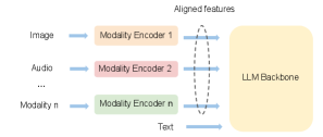
Multimodal large language model (MLLM) comprises three key parts: one or multiple modality encoders, input projectors, and a large language model backbone[36]. The Modality Encoders are designed to encode inputs from non-textual modalities into respective features, while the input projector aligns features from these modalities with the text feature space. Ultimately, the LLM backbone utilizes aligned features from various modalities and textual features as its input. Figure 1 illustrates the architecture of the MLLM. We exclude the input projector from our discussion due to its relatively minor computational demand compared to the encoder and the LLM (refer to Llava [19]). Additionally, we treat the input projector as the final layer of the modality encoder in our analysis.
Different from homogeneous LLM architecture, multimodal LLM has the following unique characteristics.
Dominant Model Size of LLM Backbone: In multimodal LLMs, the LLM backbone has a significantly larger number of parameters compared to other components such as encoders and projectors. For instance, Flamingo [4] boasts a total of 80 billion parameters, with its LLM backbone alone comprising 70 billion parameters.
Dependency between Encoders and LLM Backbone: In MLLM training, there are two types of data dependencies between encoders and LLM. During the forward pass, encoders must complete the generation of encoded features before the LLM backbone can proceed with forwarding. Conversely, in the backward pass, the LLM backbone calculates gradients before the encoders initiate the backward pass.
2.2 Bubbles in MLLM Training
Existing LLM pipeline optimizations are not model-agnostic, and fall short in MLLM training tasks. In our internal large-scale MLLM training tasks with ViT encoder and GPT backbone (over 100B parameters), we train Megatron-LM with more than 3,000 NVIDIA GPUs and observe more than 48% GPU cycle idleness when applying multiple SOTA techniques, including MegaScale [14], Zero Bubble Pipeline [24], fine-grained communication-computation overlapping [32]. We analyze the profiled timeline to identify and investigate the occurrences of GPU idleness (i.e., bubbles). Table 1 shows the total time and percentage of average training step time (5.12s) occupied by different types of bubbles.
| Bubble types | Percentage | Total time (s) |
|---|---|---|
| DP bubble (all-gather) | 3.3% | 0.167 |
| DP bubble (reduce-scatter) | 8.9% | 0.458 |
| PP bubbles (warmup) | 5.0% | 0.291 |
| PP bubbles (cooldown) | 9.2% | 0.471 |
| PP bubbles (other) | 8.7% | 0.445 |
| TP bubble | 11.2% | 0.585 |
These bubbles can be classified into three categories based on their underlying causes.
(1) Communication in Data Parallelism (DP). Data parallelism requires communication to aggregate gradients, leading to GPU idle time during the communication. Specifically, MegaScale [14] and Megatron-LM [26] use the distributed optimizer (similar to in ZeRO [25]) to save memory for large model training, which performs two collective communications (all-gather and reduce-scatter). At the start of each training step, an all-gather operation gathers updated parameters from all data parallel (DP) ranks, resulting in a DP all-gather bubble (occupying 3.3% of the training time). At the end of the training step, reduce-scatter is performed to aggregate gradients, leading to a DP reduce-scatter bubble (occupying 8.9% of the training time). It should be noted that overlapping optimization in data parallelism proposed in Megascale [14] have already been applied and above DP communications are required for the first model chunk which can not be hidden because of the nature of synchronous training [14]. Figure 2 illustrates DP bubbles that occur due to all-gather and reduce-scatter operations at the start and conclusion of each training step.

(2) Dependency in Pipeline Parallelism (PP). Despite applying pipeline send-receive overlap optimization from Megascale [14], pipeline bubbles still occur due to the inherent data dependencies between stages during the forward and backward passes. It should be noted that Zero Bubble Pipeline cannot eliminate pipeline bubbles in MLLM training, owing to the required changes in the optimizer [24] (refer to discussions in §7). Figure 2 illustrates the MLLM training pipeline schedule, which consists of three phases: warm-up (forward only), steady (one forward and one backward), and cool-down (backward only). Throughout pipeline training, three types of bubbles arise:
-
•
PP warm-up bubbles occur at all stages except the initial one due to the forward dependency of the first forward pass, averaging 5.0% of the training time.
-
•
PP cool-down bubbles occur at all stages except the initial one due to the backward dependency of the final backward pass, averaging 9.2% of the training time.
-
•
Other PP bubbles manifest at all stages except the last one due to dependencies of other forward and backward passes, occupying 8.7% of training time. For instance, PP bubbles emerge immediately after the PP warm-up phase due to the backward dependency of the initial backward pass. Additionally, in cases of imbalanced pipeline stages caused by MLLM’s heterogeneous model, there are additional pipeline bubbles not depicted in Figure 2.
(3) Communications in Tensor Parallelism (TP). Tensor parallelism entails partitioning individual model layers across multiple GPUs, necessitating communication during forward and backward passes to synchronize between GPUs. In Megatron-LM, each forward or backward pass of a transformer layer involves two all-gather and two reduce-scatter kernels [15]. Figure 3 provides a detailed view of CUDA computation and communication kernels during two GPT-175B[6] layer forward passes. In the CUDA communication stream, green kernels represent all-gather communications, while blue kernels denote reduce-scatter communications. The compute stream idles during these communications. Typically, these TP bubbles last for sub-millisecond durations, averaging around 300 s. However, during MLLM training, there are thousands of TP bubbles, totaling 11.2% of the training time.

2.3 Challenges
To minimize bubbles in MLLM training, we aim to leverage the distinct dual-component structure of MLLM, which includes encoders and the LLM backbone. We have noted two key observations. Firstly, the majority of bubbles during MLLM training tend to occur during the forward and backward passes of the LLM backbone, with around 90% of these bubbles arising from LLM communication, as indicated in Table 1. Secondly, the encoders require fewer computational operations (FLOPs) than the LLM backbone due to their smaller number of parameters[5, 8, 19, 18, 11].
In response, we propose to schedule encoder computation in LLM bubbles (occurring during communication in LLM) to reduce bubbles throughout the MLLM training process.
We identify three main challenges of scheduling encoder computation to LLM bubbles.
Challenge 1: Only a few GPUs have both encoder and LLM model states. Current training systems [38, 21] use pipeline parallelism to parallelize the MLLM as a single pipeline. Due to the dependency between the encoder and LLM, encoder layers are assigned to earlier pipeline stages, while LLM layers are assigned to later pipeline stages. Consequently, only one pipeline stage typically contains both encoder and LLM layers. To illustrate, Figure 4 demonstrates the application of 3D parallelism (DP=1, PP=4, TP=2) to parallelize MLLM across 8 GPUs, where only 2 GPUs in pipeline stage 1 possess both encoder and LLM model states. The remaining 6 GPUs are incapable of executing encoder computations during LLM bubbles because they lack encoder model states.

Challenge 2: Complex Dependencies in MLLM Training. The intricate dependencies inherent in MLLM training pose significant challenges when scheduling encoder computation within LLM bubbles. Firstly, in synchronous training, the utilization of LLM bubbles is restricted to executing the required encoder computation solely within the current training iteration (iteration dependency). Secondly, the dependency within the encoder pipeline requires scheduling the forward computation of the current encoder pipeline stage after the completion of the previous encoder stage, and scheduling the backward computation after the subsequent encoder stage concludes. Lastly, the encoder-LLM dependency entails a microbatch-level dependency, where the encoder must complete the forward pass of microbatch before the LLM pipeline initiates the forward pass of microbatch , and similarly, the encoder can commence the backward pass of microbatch after the LLM pipeline completes the backward pass of microbatch .
Challenge 3: Sub-millisecond LLM bubbles. Existing frameworks like MegaScale[14] and Megatron-LM[21] typically schedule in the unit of layers. However, bubbles in the LLM exhibit a wide range of durations, spanning from sub-milliseconds (TP bubbles) to hundreds of milliseconds (DP bubbles). For instance, TP bubbles in Figure 3 average around 300s across different LLM layers during forward and backward passes and they are too short to complete even a single encoder layer forward or backward. For example, a single ViT-22B layer typically requires around 1.4 milliseconds to complete forward propagation and 2.0 milliseconds to complete backward propagation.
3 Design Decisions and System Overview
We discuss the core design decisions that drive Optimus design and provide an overview of Optimus. The next section discusses the detailed design.
3.1 Design Decisions
Design decision 1: Colocate encoders and LLM with separate parallelism. To ensure that each GPU possesses both encoder and LLM model states, we propose assigning separate parallel plans to encoders and LLMs across all GPUs. This strategy is illustrated in Figure 5, where using parallel plan (DP=2, PP=2, TP=2) for encoders and (DP=1, PP=4, TP=2) for LLM. Each GPU retains both encoder and LLM model states, and then it becomes feasible for all GPUs to execute encoder computations during LLM bubbles. Note that colocating both the encoder and LLM states may require more GPU memory and we analyze the memory overhead in Section 4.5.

Design decision 2: Dual-Stage Dependency Management. We use two stages to handle complex dependencies in MLLM training: local scheduling and global ordering. Each encoder pipeline undergoes local scheduling, which schedules encoder computations with available LLM bubbles, adhering to the iteration-dependency and encoder-internal dependencies. Global ordering ensures microbatch-level dependency between encoders and LLM by sequencing the encoder’s ending times forward and the encoder’s starting times backward across microbatches. This involves comparing timestamps to verify encoder-LLM dependency compliance. As shown in Figure 6, local scheduling is applied independently to two encoder pipelines, maintaining iteration dependency and encoder-internal dependency. In global ordering, timestamps across all microbatches (totaling 8) are checked to confirm that encoder-LLM dependencies are met.

Design Decision 3: Schedule encoder computation at Kernel Level. Decomposing the encoder layer into kernels enables efficient utilization of sub-millisecond bubbles. However, TP communication kernels in the encoder layer compete for link bandwidth during LLM TP bubbles, causing longer time per iteration. To resolve this, we must additionally schedule encoder communication kernels during LLM compute (see Figure 7).

3.2 Optimus Overview
Optimus is a distributed training system designed for MLLM, enabling the scheduling of encoder computation within LLM bubbles to improve end-to-end training latency. To tackle challenges in Section 3.1, Optimus has two components, which are the model planner and bubble scheduler.
Model Planner. The model planner partitions encoders and the LLM backbone separately to all given GPUs (addressing Challenge 1 in §3.1). Initially, the planner determines the 3D parallelism plan () for the LLM backbone based on insights in Megatron-LM[21]. Subsequently, the planner enumerates potential 3D parallelism plans () for the encoders, considering the available GPU memory after the deployment of the LLM. With the model planner, each GPU holds both LLM and encoder model states, enabling encoder computation during LLM bubbles. The encoder and LLM model parallel plans are provided as input to the bubble scheduler, where Optimus selects parallel plans based on the output schedule with the shortest execution time.
Bubble Scheduler. Bubble scheduler is responsible for scheduling encoder computation into LLM bubbles. Given that the LLM training pipeline divides data into multiple microbatches, the scheduler schedules encoder computations on a per-microbatch basis and satisfies encoder-LLM data dependency at microbatch level (addressing Challenge 2 in §3.1). In addition, the scheduler breaks down encoder computation into kernel granularity, to enable the utilization of sub-millisecond bubbles (TP bubbles) during LLM training (addressing Challenge 3 in §3.1).
Optimus uses the model planner to devise parallel plans for both encoders and LLMs. Subsequently, for each encoder parallel plan, Optimus utilizes the bubble scheduler to generate a schedule and estimate the latency. Ultimately, Optimus selects the schedule with the shortest training time to schedule encoder computation into LLM bubbles. The workflow of Optimus is outlined in Algorithm 1.
4 Optimus Design
Section 4.1 describes how the model planer searches the parallel plans for the encoder, Section 4.2 details how the bubble scheduler exploits the coarse-grained and fined-grained bubbles through local scheduling, Section 4.3 discusses how the bubble scheduler handles encoder-LLM data dependencies through global ordering, Section 4.4 designs the bubble scheduling in multi-branch encoder models, and Section 4.5 analyzes the memory consumption of the bubble scheduling algorithm.
4.1 Model Planner
Searching separate parallel plans. Initially, the planner determines the 3D parallelism plan () for the LLM backbone based on insights in Megatron-LM[21]. Subsequently, the planner enumerates potential 3D parallelism plans (), ensuring that is a factor of and is a factor of . In practice, can reach up to 64 and up to 8 for training large language models (LLMs) [21]. Consequently, there are generally no more than 28 encoder parallel plans available, with up to 7 options for and 4 for .
Colocating encoders and LLM. To guarantee that each GPU can perform encoder computations during LLM downtime, the model planner assigns both encoder and LLM model states to every GPU. As illustrated in Figure 5, all GPUs contain model states for both the encoder (depicted in green) and the LLM (shown in red). Without such colocation, many GPUs would lack the necessary encoder model states to execute encoder computations.
Prune parallel plans based on memory constraint. As we colocate the encoder and LLM stages on GPUs, we calculate the memory requirements for both encoder and LLM states based on the chosen parallelism plan, referencing memory analysis in [15]. Plans that violate GPU memory capacity are immediately pruned.
Constructing separate microbatches. Due to the different parallel plans for encoders and LLMs, there are times more encoder pipelines than LLM pipelines for a given set of GPUs (e.g. in Figure 5). For GPUs belonging to the same LLM pipeline, there are encoder pipelines colocated. Depending on the number of microbatches utilized in LLM pipeline training, the data from these microbatches needs to be distributed among these encoder pipelines, where each encoder pipeline handles forward and backward computations for microbatch data. The model planner enumerates possible ways to partition these microbatches among the encoder pipelines. For instance, if there are 8 microbatches in the LLM training and encoder pipelines, there are a total of 7 possible partitioning options, such as , , …, .
4.2 Bubble Scheduling
Although LLM bubbles in different GPUs have different start times and duration, there is one common pattern of LLM bubbles as shown in Figure 8. There is one single big bubble (the sum of DP all-gather bubble and PP-warm bubble) before any LLM computation starts and one single big bubble (the sum of PP-cooldown bubble and reduce-scatter bubble) after all LLM computation finishes. And there are many small bubbles (PP bubbles and TP bubbles)[21, 26, 15] interleaved with LLM computation.

Design decision 2: The bubble scheduler, as described in Algorithm 2, initially engages in coarse-grained bubble exploitation by creating initial schedules that incorporate encoder computations within the bubbles positioned before and after LLM computations (line 2). However, it’s possible that these two bubbles may not allow sufficient time to complete all encoder computations, leading to some encoder computations being unscheduled within bubbles. To reduce the total training time, the bubble scheduler then executes fine-grained bubble exploitation. This involves refining the schedule by allocating encoder forward computations to the bubbles that alternate with LLM computations (line 7), followed by assigning encoder backward computations to these same bubbles (line 8). The final output of the bubble scheduler is the schedule that achieves the shortest possible runtime.
Coarse-grained bubble exploitation. For each potential data partitioning approach, the bubble scheduler initializes the schedule by scheduling encoder forward operations to occur before LLM computations and encoder backward operations to occur after LLM computations. Figure 9 illustrates the initialized schedule when there are encoder pipelines and the data partitioning approach is , i.e., 3 microbatches is allocated to the first encoder pipeline and 5 for the second encoder pipeline.

Fine-grained bubble exploitation. The OptimizeSchedule function (line 15 at Algorithm 2) refines the initial schedule through an iterative approach. Initially, the bubble scheduler employs findCritical to identify the encoder pipeline whose computation is on the critical path of the end-to-end MLLM training (line 17). Subsequently, it utilizes AssignKernels to allocate one microbatch of this encoder computation to bubbles interleaved with LLM computations (line 18). If there are sufficient bubbles available for scheduling encoder computation and encoder-LLM data dependencies are met, the bubble scheduler repeats this process. Otherwise, it returns the current optimized schedule.
When optimizing the schedule for encoder forward computation (line 7 in Algorithm 2), findCritical identifies the encoder pipeline whose forward computation is critical. As shown in the left portion of Figure 10, encoder pipeline 2’s forward computation (microbatch 8 forward) is initially on the critical path in the initial schedule. After successfully scheduling that microbatch forward to later bubbles, encoder pipeline 1 assumes the critical path position. This iterative process leads to a reduction in the end-to-end MLLM training time after each step. Similarly, encoder pipelines whose backward computation is critical are illustrated in the right portion of Figure 10. After each step, the bubble scheduler must verify if it still satisfies the encoder-LLM data dependency before proceeding with the next steps.

When scheduling encoder computation to bubbles interleaved with LLM compute (AssignKernels at line 18), the bubble scheduler decomposes the encoder computation into kernel granularity and schedules these kernels based on the duration of the bubble. For each bubble, the bubble scheduler schedules multiple kernels while ensuring that the total execution time of these kernels is within the bubble duration. Additionally, the bubble scheduler must satisfy the encoder’s internal data dependencies. As illustrated in Figure 11, device 1 holds the first two layers of the encoder, while device 2 holds the next two layers. When scheduling kernels during the forward pass, device 2 can only utilize bubbles that occur after device 1 completes its forward pass to execute encoder computation. For the forward computation, the bubble scheduler schedules encoder computation from upstream encoder pipeline stages to downstream encoder pipeline stages. Conversely, for backward computation, the bubble scheduler schedules encoder computation in the reverse order. While each encoder layer also includes communication kernels, the scheduler ensures that these kernels are not assigned to TP bubbles that occur during LLM communication. Instead, the scheduler identifies long-duration computation kernels within the LLM layers and overlaps them with encoder communication kernels. As the LLM and encoder layers alternately perform computation and communication tasks, they make efficient use of GPU bandwidth and Streaming Multiprocessors (SMs). This design strategy helps to minimize resource contention and improves overall GPU utilization[16].

Complexity. Our bubble scheduling algorithm has low complexity. Given GPUs and the number of prime factors of is , the search space of parallel plans is . The number of microbatch partitioning is . Hence, the complexity for scheduling bubbles is . For our experimented settings, it usually takes around several minutes to calculate the optimal schedule (see §5.3.2), which is also a one-time cost.
4.3 Address Encoder-LLM dependency
| Symbol | Description |
|---|---|
| LLM Data Parallel Size | |
| Encoder Data Parallel Size | |
| Number of microbatches in LLM training | |
| Encoder input data microbatch | |
| LLM input activations for microbatch | |
| LLM output gradients for microbatch | |
| Forward dependency point for microbatch | |
| Backward dependency point for microbatch |
The model planner provides different parallel strategies for encoders and LLM backbone, including the number of microbatches, resulting in complex data dependencies both between and within the encoder and LLM. Also, the communication and computation of the encoder and LLM are executed by interleaving, and this may introduce additional pipeline bubbles, if not orchestrated effectively, intensifying the complexity of dependencies in the system.
The bubble scheduler addresses encoder-LLM dependencies at the microbatch level by examining the encoder-LLM forward and backward dependency points for each microbatch . These dependency points, denoted as and respectively, represent the time when the LLM requires the corresponding activations (output by the encoder) for forward propagation, and when the LLM generates the corresponding gradients (input for the encoder) during backward propagation. To ensure the satisfaction of encoder-LLM dependencies, the bubble scheduler employs two functions: GetEncLLMDep (line 3 at Algorithm 2) and CheckEncLLMDep (line 19 at Algorithm 2), as described below.
GetEncLLMDep gets encoder-LLM forward and backward dependency points.
Given that the interleaved 1F1B schedule [21] stands out as one of the most efficient pipeline schedules for LLM training, we delve into the specifics of the data dependency points and within this schedule. The top illustration in Figure 12 depicts an instance of the interleaved 1F1B schedule featuring two model chunks. Here, the forward dependency points denote the instances when the first pipeline stage (device 1) commences forward execution for the first model chunk (depicted in dark blue), while the backward dependency points signify the moments when the first pipeline stages (device 1) complete backward execution for the first model chunk (depicted in dark green).
We observe that deferring forward data dependency points for the last four microbatches ( through ) is feasible without exerting any adverse effects on the overall pipeline latency. To accomplish this, we can adjust the number of warmup microbatches at each pipeline stage, as illustrated in the bottom portion of Figure 12. This adjustment enables the bubble scheduler to leverage bubbles during the phase transition from the warmup phase to the 1F1B-steady phase for scheduling encoder forward computation when optimizing initial schedules. GetEncLLMDep yields the adjusted forward and backward data dependency points for 1F1B interleave schedules.

CheckEncLLMDep verifies the satisfaction of microbatch-level encoder-LLM dependencies. By considering the scheduled encoder computation into bubbles, the bubble scheduler estimates when the encoder finishes the forward pass for microbatches distributed over different encoder pipelines. The bubble scheduler sorts these finishing times in ascending order as (global ordering), representing when the encoder forward operation ends for microbatch involved in LLM pipeline training. The forward dependency for encoder-LLM is considered met if the encoder completes its forward operation before the specified timepoint () for all microbatches (). Similarly, the backward dependency is satisfied if the encoder’s backward operation begins no earlier than the timepoint () for each microbatch (). CheckEncLLMDep returns true when it confirms that both the forward and backward dependencies are successfully met. To illustrate this, Figure 13 provides an example of evaluating encoder-LLM dependency with two encoder pipelines, each handling four microbatches. The order in which the encoder completes its forward pass dictates how the activations are used in the LLM pipeline: activations from encoder pipeline 1 are designated as the 1st, 3rd, 7th, and 8th microbatches, while activations from encoder pipeline 2 are used as the 2nd, 4th, 5th, and 6th microbatches. The bubble scheduler then verifies microbatch-level dependency by ensuring that each encoder’s forward operation concludes before the start of the corresponding LLM forward pass and that each encoder’s backward operation does not commence until after the LLM has ended, for each microbatch.

When dependencies are satisfied, the bubble scheduler integrates necessary peer-to-peer (P2P) communications into the training schedule between the last stage of the encoder pipeline and the first stage of the LLM pipeline. For instance, if encoder pipeline completes the forward pass for microbatch , the scheduler will insert a P2P send (sending activations) at the last stage of encoder pipeline and a P2P receive (receiving activations) at the first stage of the LLM pipeline. Similarly, when the LLM pipeline completes the backward pass for microbatch , the scheduler adds a P2P send (sending gradients) at the first stage of the LLM pipeline and a P2P receive (receiving gradients) at the last stage of encoder pipeline . In the scenario depicted in Figure 13, the scheduler inserts 8 pairs of P2P send-receive at devices 1 and 2 to manage the dependencies between encoder pipeline 1 and the LLM pipeline, with 4 pairs allocated for forward dependencies and 4 pairs for backward dependencies. Likewise, an additional 8 pairs of P2P send-receive are inserted at devices 3 and 4 to address the dependencies between encoder pipeline 2 and the LLM pipeline.
4.4 Multi-Branch Encoder Scheduling
To support MLLM with multiple encoders[7, 35], the model planner applies an encoder parallelism plan . independently for each encoder. For pipeline parallelism, layers within each encoder are divided into stages (as illustrated in Figure 14). Each layer of every encoder is then parallelized according to . The bubble scheduler breaks down the layers of distinct encoders into kernel-level granularity and arranges their scheduling as if these kernels were part of a single encoder. This is because the encoders within MLLM operate independently, without any data dependencies between them.

4.5 Memory Analysis
When utilizing GPUs for MLLM training, the model planner requires replicated encoder model states and replicated LLM model states based on parallel plans. Suppose the number of parameters in the encoder is and the number of parameters in the LLM is , with each parameter requiring bytes of memory. The average GPU memory usage for storing model states is calculated as follows:
In comparison to existing 3D parallel training solutions, where , the estimated memory overhead can be expressed as:
With a larger value of , there is a higher memory overhead due to more replicated encoder model states. However, this results in less complex encoder internal dependencies during scheduling (indicated by a smaller ). Model planner filters the encoder parallel plans based on the estimated memory usage , ensuring adherence to GPU memory constraints. In practice, the memory overhead typically amounts to less than 12% in our evaluation (§5.3.1) because is small (e.g., the largest vision encoder has 22 billion parameters [10]) and is small (e.g., when using parameters and gradients with distributed optimizer[1]).
5 Evaluation
We have developed Optimus based on the open-source Megatron-LM framework [1] and evaluate Optimus on training large-scale mulitimodal LLMs.
5.1 Methodology
Testbed. We conduct our experiments in a production training cluster with thousands of NVIDIA Hopper GPUs. Each GPU has 80GB memory and 989TFLOPS computing performance. The intra-server connection is NVLink and the inter-server connection is a high-bandwidth RDMA network.
MLLM models. We examine the performance of Optimus using various sizes of image encoders and LLM backbones. The image encoders include three sizes: ViT-22B [10], ViT-11B, and ViT-5B, which are scaled-down versions of ViT-22B with smaller hidden sizes. For the language models, we employ two sizes: LLAMA-70B [31] and GPT-175B [6]. Appendix A includes detailed model configurations.
Baselines. We use three open-sourced MLLM training systems with one strawman method as our baselines for comparison.
PyTorch FSDP [37]: FSDP is a distributed data-parallel training module designed to scale PyTorch models across multiple GPUs with minimal code changes. It shards the model across GPUs, runs to collect all shards from all ranks to recover the full parameter for forward and backward computation, and runs to synchronize gradients.
Alpa [38]: Alpa is a compiler system for distributed DL training that automatically generates parallel execution plans covering 3D parallelisms.
Megatron-LM [21]: Megatron-LM is a state-of-the-art LLM training framework that integrates 3D parallelism techniques. Megatron-LM is designed for symmetric transformer models, and we place multimodal encoders to the preprocess in the first pipeline stage to adapt to MLLM training.
Megatron-LM balanced: In this strawman method, we balance the layer partitioning among different pipeline stages with an interleaved 1F1B pipeline schedule. Considering the heterogeneity in MLLM submodules, we use a dynamic programming algorithm to assign different layers of submodules to pipeline stages and achieve approximately the same computation amount. The DP algorithm is a simplified version of Alpa’s inter-operator DP algorithm and is included in Appendix B.
We use iteration time and Model Flops Utilization (MFU) [9] as the performance metrics. The reported performance numbers are averaged over 300 training iterations after a warm-up of 10 iterations. The detailed Megatron-LM configurations across experiments are included in Appendix D.
5.2 End-to-End Performance
5.2.1 Weak-Scaling Experiment
Experiment Setup. To study the ability to train large models, we follow common ML practice to scale the model size along with the number of GPUs. We evaluate the weak-scaling training performance of Optimus and baselines based on model configurations in Table 3.
| Name | Encoder | LLM | #GPUs | Batch Size |
|---|---|---|---|---|
| Model A | ViT-11B | LLAMA-70B | 64 | 32 |
| Model B | ViT-22B | LLAMA-70B | 128 | 64 |
| Model C | ViT-11B | GPT-175B | 256 | 128 |
| Model D | ViT-22B | GPT-175B | 512 | 256 |
Results. Figure 15 presents a comparison between Optimus and baseline methods across various sizes of MLLM. Optimus achieves a speedup of up to 1.22 compared to Megatron-LM and 1.18 compared to the Megatron-LM balanced. Alpa and FSDP face GPU out-of-memory (OOM) issues with these models.

For our comparison with Alpa and FSDP, we crafted a modest MLLM that includes ViT-3B and GPT-11B, where Optimus demonstrates a 3.09 speedup compared to Alpa and a 15.1% improvement over FSDP, as detailed in Table 4. Further setup details can be found in Appendix C.
| Alpa | FSDP | Megatron-LM | Megatron-LM balanced | Optimus | |
| Time (s) | 8.61 | 3.20 | 3.42 | 3.04 | 2.78 |
5.2.2 Strong-Scaling Experiment
Experiment setup. We assess the strong-scaling training performance of Optimus and Megatron-based baselines using the ViT-22B+GPT-175B model. Following [14], we progressively increase the number of GPUs used (1536, 2048, and 3172) while keeping the batch size constant at 1536.
Results. Table 5 compares training performance between Optimus and Megatron-LM based baselines with an increasing number of GPUs. Optimus reduces iteration time by up to 21.3% compared to Megatron-LM, and by up to 20.5% compared to the Megatron-LM balanced. With the increase in GPU count, Optimus exhibits a more pronounced speedup relative to baseline solutions. This enhanced performance is anticipated since the constant batch size coupled with an increased GPU count escalates the bubble ratio, enabling Optimus to allocate a larger proportion of encoder computations to LLM bubbles. It is also evident that Optimus maintains a stable MFU, whereas the baseline MFU declines when scaling to more GPUs.
| Batch Size | Method | GPUs | Iteration Time (s) | MFU | Aggregate PFlops/s | ||||||||||||
|---|---|---|---|---|---|---|---|---|---|---|---|---|---|---|---|---|---|
| 1536 | Megatron-LM |
|
|
|
|
||||||||||||
| Megatron-LM balanced |
|
|
|
|
|||||||||||||
| Optimus |
|
|
|
|
5.2.3 Multi-Encoder MLLM Experiment
Experiment setup. We assess the training performance of Optimus and Megatron-LM on multi-encoder MLLMs on 512 GPUs with batch size 256 (refer to Table 6). The Megatron-LM balanced baseline was excluded from this evaluation since its dynamic programming algorithm is designed to partition layers solely in MLLMs with a single encoder (linear model configuration).
| Name | Encoder-1 | Encoder-2 | LLM |
|---|---|---|---|
| DualEnc(11B, 5B) | ViT-11B | ViT-5B | GPT-175B |
| DualEnc(22B, 5B) | ViT-22B | ViT-5B | GPT-175B |
| DualEnc(22B, 11B) | ViT-22B | ViT-11B | GPT-175B |
Results. Figure 16 illustrates the average iteration times of Optimus compared to the Megatron-LM. Optimus achieves a speedup of up to 1.25, 1.26 and 1.27 on these MLLMs. This increased speedup by Optimus can be attributed to the Megatron-LM’s approach of placing all encoders in the first pipeline stage, which leads to a more severe pipeline imbalance due to the larger total parameter count of the encoders.

5.3 Microbenchmarks
5.3.1 Optimus Memory
Experiment setup. We measure the GPU memory consumption of Optimus and baselines during the training of MLLMs of different sizes (listed in Table 3).
Results. As shown in Figure 17, Optimus presents a maximum GPU memory overhead of 12% when compared to the most memory-efficient baseline across various models. It is noted that Optimus uses less GPU memory than both baselines for model C and Megatron-LM balanced for model D. This discrepancy stems from the baseline’s strategy of distributing computational loads across different pipeline stages, which can lead to memory imbalances due to varying hidden sizes in the encoder and LLM layers.

5.3.2 Bubble Scheduler Algorithm
Experiment Setup. We executed the bubble scheduler algorithm on a single CPU core to compute the bubble schedule for training the ViT-22B+GPT-175B model with a global batch size of 1536 across an increasing number of GPUs (1536, 2048, and 3172), the same as the setting described in the strong-scaling experiment (Section 5.2.2). To evaluate the efficacy of the bubble scheduler algorithm, we developed a metric called scheduling efficiency, which quantifies the percentage of encoder computations that can be effectively scheduled within the LLM bubble. We report two efficiency metrics derived from simulations: , observed when utilizing only coarse-grained bubble exploitation, and , observed when both coarse-grained and fine-grained bubble exploitations are activated (see §4.2). Additionally, we report the runtime of the bubble scheduler algorithm.
Results. Table 7 illustrates that the bubble scheduler achieves higher scheduling efficiencies, and , when operating with an increased number of GPUs for MLLM training. This improvement is attributed to the constant batch size of 1536, where the number of microbatches allocated to each LLM pipeline is reduced (32, 24, 16) as the number of GPUs increases (1536, 2048, 3172). Consequently, the LLM pipeline exhibits a higher bubble ratio due to the fixed durations of DP bubble and PP-warmup/PP-cooldown bubbles, while the total time for the end-to-end LLM pipeline decreases. Moreover, enabling fine-grained bubble exploitation can yield up to a 1.67 increase in efficiency compared to . It is noted that the runtime of the bubble scheduler algorithm tends to decrease as the number of microbatches in the LLM pipeline reduces, due to fewer microbatch partitioning options (see algorithm complexity analysis in 4.2).
| Settings | #Microbatch | Runtime (s) | ||
|---|---|---|---|---|
| 1536-GPU | 32 | 34.3% | 57.5% | 322.2 |
| 2048-GPU | 24 | 45.8% | 69.3% | 89.6 |
| 3172-GPU | 16 | 68.7% | 85.0% | 15.1 |
6 Discussion
Complex computation graph. Optimus focuses on the bubble scheduling on typical MLLM model architecture, which consists of multimodal encoders followed by one LLM. We may further explore the bubble scheduling for complex MLLM computation graphs. A new partitioning algorithm is required to divide the computation graph into the backbone pipeline schedule and the bubble-filling workload. And the bubble scheduling algorithm of Optimus can be easily extended to the partitioned computation graph.
Other pipeline schedules. We use a widely-used Megatron-LM interleaved 1F1B pipeline schedule for MLLM training. However, there exist other pipeline schedules (e.g., Chimera [17] and zero-bubble pipeline [24]) that may have superior performance in certain scenarios. The bubble scheduling of Optimus is orthogonal to these pipeline schedule optimizations, and Optimus can be applied to other pipeline schedules when the specific encoder-LLM dependency is analyzed and addressed.
Online scheduling. For simplicity, our bubble scheduling algorithm omits the consideration of fluctuating runtime execution time of CUDA kernels. We collect performance statistics such as CUDA kernel execution time to identify the bubble occurrence and duration during a training step for the bubble scheduler, assuming the behavior remains the same in the following training steps. The bubble scheduling may be sub-optimal when there is a significant deviation in the predicted pipeline execution time. For instance, the insertion of encoder computation into a non-bubble position may result in larger, unexpected pipeline bubbles with altered execution orders. A potential solution is to use real-time performance monitoring, and dynamically fine-tune the bubble scheduling.
7 Related works
Multi-modal training. Pytorch FSDP training [37] supports only data parallelism and is less efficient than hybrid parallel strategies. Alpa [38] automates parallelism for various models but falls short by not supporting state-of-the-art 1F1B-interleave pipeline parallelism [21] and requiring more memory than the optimized Megatron-LM framework [26], also missing opportunities in pipeline optimization due to its unified view of encoders and decoders. DistMM [13] provides solutions to orchestrating multiple parallel encoders but it is designed for contrastive learning and overlooks the decoder, leaving a gap in comprehensive training efficiency.
Bubble reducing. Previous efforts in reducing “bubbles” have approached the problem from various angles. The 1F1B-interleave pipeline [21] technique minimizes bubbles by chunking the model and alternating these chunks across different stages, whereas the Zero bubble pipeline [24] approach further granulates backward pass computations to eliminate bubbles. However, in practice, the Zero bubble pipeline schedule cannot completely remove all pipeline bubbles because it requires changes to the optimizer, which raises concerns about end-to-end model convergence. Sarathi [3] splits sequence into smaller chunks to do multi-step prefilling and thus reduce pipeline bubble in LLM inference. On the other hand, asynchronous tensor parallelism [27] and Google’s overlapping technique [32] aim to overlap tensor parallelism communication with computation but are limited by specific hardware configurations and struggle to maintain full overlap as computing capabilities advance.
Bubble exploiting. Pipefisher [23] leverages pipeline bubbles across multiple training steps to complete the K-FAC, whereas our method operates within a single synchronized training step, focusing on immediate optimization. Hydro’s Bubble Squeezer [12] utilizes GPT model bubbles for independent tasks like hyperparameter tuning which can not enhance the performance of the training steps themselves. Bamboo [30] employs pipeline bubbles for redundant computations to mitigate the impact of preemption in training on volatile instances, based on the assumption that later pipeline stages host more layers, which often does not hold in large language model (LLM) training scenarios.
8 Conclusion
We present Optimus, a distributed MLLM training system that enables the scheduling of encoder computation within LLM bubbles to reduce end-to-end MLLM training time. To reduce GPU bubbles during MLLM training, Optimus partitions multimodal encoders and the LLM backbone, and schedules encoder computation in LLM bubbles. We search for the optimal parallelism plan for the encoders with the consideration of memory and computation resource constraints, which balances the encoder computation among GPUs for bubble filling. Optimus further employs a bubble scheduling algorithm to address encoder-LLM dependency and select the optimal schedule for filling kernel-level encoder computation into sub-millisecond LLM bubbles. Our extensive experiments demonstrate that Optimus can accelerate MLLM training by 20.5%-21.3% with ViT-22B and GPT-175B model over 3072 GPUs compared to baselines and significantly outperforms existing MLLM training systems by 20.3% on average.
References
- [1] GitHub - NVIDIA/Megatron-LM: Ongoing research training transformer models at scale — github.com. https://github.com/NVIDIA/Megatron-LM. [Accessed 07-05-2024].
- [2] Aishwarya Agrawal, Jiasen Lu, Stanislaw Antol, Margaret Mitchell, C. Lawrence Zitnick, Dhruv Batra, and Devi Parikh. Vqa: Visual question answering, 2016.
- [3] Amey Agrawal, Ashish Panwar, Jayashree Mohan, Nipun Kwatra, Bhargav S Gulavani, and Ramachandran Ramjee. Sarathi: Efficient llm inference by piggybacking decodes with chunked prefills. arXiv preprint arXiv:2308.16369, 2023.
- [4] Jean-Baptiste Alayrac, Jeff Donahue, Pauline Luc, Antoine Miech, Iain Barr, Yana Hasson, Karel Lenc, Arthur Mensch, Katherine Millican, Malcolm Reynolds, et al. Flamingo: a visual language model for few-shot learning. Advances in neural information processing systems, 35:23716–23736, 2022.
- [5] Jinze Bai, Shuai Bai, Shusheng Yang, Shijie Wang, Sinan Tan, Peng Wang, Junyang Lin, Chang Zhou, and Jingren Zhou. Qwen-vl: A versatile vision-language model for understanding, localization, text reading, and beyond, 2023.
- [6] Tom Brown, Benjamin Mann, Nick Ryder, Melanie Subbiah, Jared D Kaplan, Prafulla Dhariwal, Arvind Neelakantan, Pranav Shyam, Girish Sastry, Amanda Askell, et al. Language models are few-shot learners. Advances in neural information processing systems, 33:1877–1901, 2020.
- [7] Jiawei Chen and Chiu Man Ho. Mm-vit: Multi-modal video transformer for compressed video action recognition, 2021.
- [8] Jun Chen, Deyao Zhu, Xiaoqian Shen, Xiang Li, Zechun Liu, Pengchuan Zhang, Raghuraman Krishnamoorthi, Vikas Chandra, Yunyang Xiong, and Mohamed Elhoseiny. Minigpt-v2: large language model as a unified interface for vision-language multi-task learning, 2023.
- [9] Aakanksha Chowdhery, Sharan Narang, Jacob Devlin, Maarten Bosma, Gaurav Mishra, Adam Roberts, Paul Barham, Hyung Won Chung, Charles Sutton, Sebastian Gehrmann, et al. Palm: Scaling language modeling with pathways. Journal of Machine Learning Research, 24(240):1–113, 2023.
- [10] Mostafa Dehghani, Josip Djolonga, Basil Mustafa, Piotr Padlewski, Jonathan Heek, Justin Gilmer, Andreas Peter Steiner, Mathilde Caron, Robert Geirhos, Ibrahim Alabdulmohsin, et al. Scaling vision transformers to 22 billion parameters. In International Conference on Machine Learning, pages 7480–7512. PMLR, 2023.
- [11] Danny Driess, Fei Xia, Mehdi S. M. Sajjadi, Corey Lynch, Aakanksha Chowdhery, Brian Ichter, Ayzaan Wahid, Jonathan Tompson, Quan Vuong, Tianhe Yu, Wenlong Huang, Yevgen Chebotar, Pierre Sermanet, Daniel Duckworth, Sergey Levine, Vincent Vanhoucke, Karol Hausman, Marc Toussaint, Klaus Greff, Andy Zeng, Igor Mordatch, and Pete Florence. Palm-e: An embodied multimodal language model, 2023.
- [12] Qinghao Hu, Zhisheng Ye, Meng Zhang, Qiaoling Chen, Peng Sun, Yonggang Wen, and Tianwei Zhang. Hydro:Surrogate-Based hyperparameter tuning service in datacenters. In 17th USENIX Symposium on Operating Systems Design and Implementation (OSDI 23), pages 757–777, 2023.
- [13] Jun Huang, Zhen Zhang, Shuai Zheng, Feng Qin, and Yida Wang. Distmm: Accelerating distributed multimodal model training. In NSDI 2024: 21st USENIX Symposium on Networked Systems Design and Implementation, 2024.
- [14] Ziheng Jiang, Haibin Lin, Yinmin Zhong, Qi Huang, Yangrui Chen, Zhi Zhang, Yanghua Peng, Xiang Li, Cong Xie, Shibiao Nong, et al. Megascale: Scaling large language model training to more than 10,000 gpus. arXiv preprint arXiv:2402.15627, 2024.
- [15] Vijay Anand Korthikanti, Jared Casper, Sangkug Lym, Lawrence McAfee, Michael Andersch, Mohammad Shoeybi, and Bryan Catanzaro. Reducing activation recomputation in large transformer models. Proceedings of Machine Learning and Systems, 5, 2023.
- [16] Shen Li, Yanli Zhao, Rohan Varma, Omkar Salpekar, Pieter Noordhuis, Teng Li, Adam Paszke, Jeff Smith, Brian Vaughan, Pritam Damania, and Soumith Chintala. Pytorch distributed: Experiences on accelerating data parallel training, 2020.
- [17] Shigang Li and Torsten Hoefler. Chimera: efficiently training large-scale neural networks with bidirectional pipelines. In Proceedings of the International Conference for High Performance Computing, Networking, Storage and Analysis, pages 1–14, 2021.
- [18] Haotian Liu, Chunyuan Li, Yuheng Li, Bo Li, Yuanhan Zhang, Sheng Shen, and Yong Jae Lee. Llava-next: Improved reasoning, ocr, and world knowledge, January 2024.
- [19] Haotian Liu, Chunyuan Li, Qingyang Wu, and Yong Jae Lee. Visual instruction tuning, 2023.
- [20] Kenneth Marino, Mohammad Rastegari, Ali Farhadi, and Roozbeh Mottaghi. Ok-vqa: A visual question answering benchmark requiring external knowledge. In Proceedings of the IEEE/cvf conference on computer vision and pattern recognition, pages 3195–3204, 2019.
- [21] Deepak Narayanan, Mohammad Shoeybi, Jared Casper, Patrick LeGresley, Mostofa Patwary, Vijay Korthikanti, Dmitri Vainbrand, Prethvi Kashinkunti, Julie Bernauer, Bryan Catanzaro, et al. Efficient large-scale language model training on gpu clusters using megatron-lm. In Proceedings of the International Conference for High Performance Computing, Networking, Storage and Analysis, pages 1–15, 2021.
- [22] OpenAI(2023). Gpt-4v(ision) system card, 2023.
- [23] Kazuki Osawa, Shigang Li, and Torsten Hoefler. Pipefisher: Efficient training of large language models using pipelining and fisher information matrices. Proceedings of Machine Learning and Systems, 5, 2023.
- [24] Penghui Qi, Xinyi Wan, Guangxing Huang, and Min Lin. Zero bubble pipeline parallelism, 2023.
- [25] Samyam Rajbhandari, Jeff Rasley, Olatunji Ruwase, and Yuxiong He. Zero: Memory optimizations toward training trillion parameter models. In SC20: International Conference for High Performance Computing, Networking, Storage and Analysis, pages 1–16. IEEE, 2020.
- [26] Mohammad Shoeybi, Mostofa Patwary, Raul Puri, Patrick LeGresley, Jared Casper, and Bryan Catanzaro. Megatron-lm: Training multi-billion parameter language models using model parallelism. CoRR, abs/1909.08053, 2019.
- [27] Siddharth Singh, Zack Sating, and Abhinav Bhatele. Communication-minimizing asynchronous tensor parallelism, 2023.
- [28] Umut Sulubacak, Ozan Caglayan, Stig-Arne Grönroos, Aku Rouhe, Desmond Elliott, Lucia Specia, and Jörg Tiedemann. Multimodal machine translation through visuals and speech. Machine Translation, 34:97–147, 2020.
- [29] Gemini Team, Rohan Anil, Sebastian Borgeaud, Yonghui Wu, Jean-Baptiste Alayrac, Jiahui Yu, Radu Soricut, Johan Schalkwyk, Andrew M Dai, Anja Hauth, et al. Gemini: a family of highly capable multimodal models. arXiv preprint arXiv:2312.11805, 2023.
- [30] John Thorpe, Pengzhan Zhao, Jonathan Eyolfson, Yifan Qiao, Zhihao Jia, Minjia Zhang, Ravi Netravali, and Guoqing Harry Xu. Bamboo: Making preemptible instances resilient for affordable training of large DNNs. In 20th USENIX Symposium on Networked Systems Design and Implementation (NSDI 23), pages 497–513, 2023.
- [31] Hugo Touvron, Louis Martin, Kevin Stone, Peter Albert, Amjad Almahairi, Yasmine Babaei, Nikolay Bashlykov, Soumya Batra, Prajjwal Bhargava, Shruti Bhosale, et al. Llama 2: Open foundation and fine-tuned chat models. arXiv preprint arXiv:2307.09288, 2023.
- [32] Shibo Wang, Jinliang Wei, Amit Sabne, Andy Davis, Berkin Ilbeyi, Blake Hechtman, Dehao Chen, Karthik Srinivasa Murthy, Marcello Maggioni, Qiao Zhang, et al. Overlap communication with dependent computation via decomposition in large deep learning models. In Proceedings of the 28th ACM International Conference on Architectural Support for Programming Languages and Operating Systems, Volume 1, pages 93–106, 2022.
- [33] xAI. Grok-1.5 vision preview, 2024.
- [34] Shaowei Yao and Xiaojun Wan. Multimodal transformer for multimodal machine translation. In Proceedings of the 58th annual meeting of the association for computational linguistics, pages 4346–4350, 2020.
- [35] Zhewen Yu, Jin Wang, Liang-Chih Yu, and Xuejie Zhang. Dual-encoder transformers with cross-modal alignment for multimodal aspect-based sentiment analysis. In Proceedings of the 2nd Conference of the Asia-Pacific Chapter of the Association for Computational Linguistics and the 12th International Joint Conference on Natural Language Processing (Volume 1: Long Papers), pages 414–423, 2022.
- [36] Duzhen Zhang, Yahan Yu, Chenxing Li, Jiahua Dong, Dan Su, Chenhui Chu, and Dong Yu. Mm-llms: Recent advances in multimodal large language models. arXiv preprint arXiv:2401.13601, 2024.
- [37] Yanli Zhao, Andrew Gu, Rohan Varma, Liang Luo, Chien-Chin Huang, Min Xu, Less Wright, Hamid Shojanazeri, Myle Ott, Sam Shleifer, et al. Pytorch fsdp: experiences on scaling fully sharded data parallel. arXiv preprint arXiv:2304.11277, 2023.
- [38] Lianmin Zheng, Zhuohan Li, Hao Zhang, Yonghao Zhuang, Zhifeng Chen, Yanping Huang, Yida Wang, Yuanzhong Xu, Danyang Zhuo, Eric P Xing, et al. Alpa: Automating inter-and Intra-Operator parallelism for distributed deep learning. In 16th USENIX Symposium on Operating Systems Design and Implementation (OSDI 22), pages 559–578, 2022.
- [39] Deyao Zhu, Jun Chen, Xiaoqian Shen, Xiang Li, and Mohamed Elhoseiny. Minigpt-4: Enhancing vision-language understanding with advanced large language models. arXiv preprint arXiv:2304.10592, 2023.
Appendix A MLLM model configurations
Here we list all the the MLLM configurations used in the evaluation experiments of Optimus. ViT encoder configurations can be found in Table 8. LLM backbone configuration can be found in Table 9. In all experiments, we use sequence length 2048.
| Models | Width | Depth | MLP dimension | Heads | Attention head dimension | Params |
|---|---|---|---|---|---|---|
| ViT-3B | 2304 | 48 | 9216 | 18 | 128 | 3B |
| ViT-5B | 3072 | 48 | 12288 | 24 | 128 | 5.5B |
| ViT-10B | 4096 | 48 | 16384 | 32 | 128 | 10B |
| ViT-22B | 6144 | 48 | 24576 | 48 | 128 | 22B |
| Models | Width | Depth | Heads | Attention-head dimension | Params |
|---|---|---|---|---|---|
| GPT-11B | 3072 | 80 | 24 | 128 | 11B |
| LLAMA-70B | 8192 | 80 | 64 | 128 | 70B |
| GPT-175B | 12288 | 96 | 96 | 128 | 175B |
Appendix B Megatron-LM balanced DP algorithm
We employ a dynamic programming (DP) algorithm to assign layers to different virtual stages for the Megatron 1F1B-interleaved schedule [21]. Following Alpa [38], the DP algorithm aims to minimize the latency of the slowest stage to reduce the end-to-end latency of the pipeline schedule. Given a pipeline parallel size of and model chunks configured, the DP algorithm seeks to minimize the latency of the slowest virtual stage. It determines the optimal layer partition strategy that distributes layers across these virtual stages.
We define the function to represent the maximum latency of a single virtual stage when the first virtual stages. The computation begins with , where denotes the execution time of the -th layer (estimated based on FLOPs). The optimal structure of is:
For a MLLM model with layers, the layer partition strategy is determined by calculating and recording the partitioning results to find the optimal solution. This ensures that the latency of the longest virtual stage, , is minimized across all virtual stages in a 1F1B-interleaved pipeline schedule. The dynamic programming algorithm described above is suitable for MLLM configurations with a single encoder, where encoder layers and LLM layers follow a linear structure. However, this DP algorithm does not apply to MLLM models that feature multiple encoders, as these encoders do not have data dependencies among each other.
Appendix C Comparison of Training Performance between Optimus, Alpa, and FSDP.
Experiment setup. To facilitate a comparison with Alpa and FSDP, we constructed a modest MLLM consisting of ViT-3B and GPT-11B, with specific configurations provided in Appendix A. We assessed the training performance using 8 NVIDIA A100 GPUs, as we encountered issues with the CUDA library when attempting to run Alpa on NVIDIA Hopper GPUs. The global batch size was set at 16, and the sequence length was 2048.
Results: According to Table 10, Optimus achieves a 3.09 speedup over Alpa and a 15.1% improvement over FSDP.
| Alpa | FSDP | Megatron-LM | Megatron-LM balanced | Optimus | |
| Time (s) | 8.61 | 3.20 | 3.42 | 3.04 | 2.78 |
Appendix D Detailed configurations for Megatron-LM based baselines
D.1 Weak-scaling experiment
Table 11 shows detailed configurations for Megatron-LM based baselines in the weak scaling experiment.
| Model | Method | GPUs | Microbatch size | Parallel configurations |
|---|---|---|---|---|
| Model A | Megatron-LM | 64 | 2 | (DP=2, PP=4, TP=8) |
| Megatron-LM balanced | (DP=2, PP=4, TP=8, V=6) | |||
| Model B | Megatron-LM | 128 | (DP=4, PP=4, TP=8) | |
| Megatron-LM balanced | (DP=4, PP=4, TP=8, V=6) | |||
| Model C | Megatron-LM | 256 | (DP=4, PP=8, TP=8) | |
| Megatron-LM balanced | (DP=4, PP=8, TP=8, V=12) | |||
| Model D | Megatron-LM | 512 | (DP=8, PP=8, TP=8) | |
| Megatron-LM balanced | (DP=8, PP=8, TP=8, V=12) |
D.2 Strong-scaling experiment
Table 12 shows detailed configurations for Megatron-LM based baselines in the strong scaling experiment.
| Model | Method | GPUs | Microbatch size | Parallel configurations |
|---|---|---|---|---|
| Model D | Megatron-LM | 1536 | 2 | (DP=24, PP=8, TP=8) |
| Megatron-LM balanced | (DP=24, PP=8, TP=8, V=12) | |||
| Megatron-LM | 2048 | (DP=32, PP=8, TP=8) | ||
| Megatron-LM balanced | (DP=32, PP=8, TP=8, V=12) | |||
| Megatron-LM | 3072 | (DP=48, PP=8, TP=8) | ||
| Megatron-LM balanced | (DP=48, PP=8, TP=8, V=12) |
D.3 Multi-encoder MLLM experiment
In multi-encoder MLLM experiment, we use (DP=8, TP=8, PP=8) and configure microbatch size as 2 for Megatron-LM for all MLLM models.