This paper was converted on www.awesomepapers.org from LaTeX by an anonymous user.
Want to know more? Visit the Converter page.

Optimum-statistical Collaboration Towards General and Efficient Black-box Optimization

Wenjie Li The two authors have contributed equally to this paper Department of Statistics, Purdue University Chi-Hua Wang * Department of Statistics, Purdue University Guang Cheng Department of Statistics, University of California Los Angeles Qifan Song Department of Statistics, Purdue University
Abstract

In this paper, we make the key delineation on the roles of resolution and statistical uncertainty in hierarchical bandits-based black-box optimization algorithms, guiding a more general analysis and a more efficient algorithm design. We introduce the optimum-statistical collaboration, an algorithm framework of managing the interaction between optimization error flux and statistical error flux evolving in the optimization process. We provide a general analysis of this framework without specifying the forms of statistical error and uncertainty quantifier. Our framework and its analysis, due to their generality, can be applied to a large family of functions and partitions that satisfy different local smoothness assumptions and have different numbers of local optimums, which is much richer than the class of functions studied in prior works. Our framework also inspires us to propose a better measure of the statistical uncertainty and consequently a variance-adaptive algorithm VHCT. In theory, we prove the algorithm enjoys rate-optimal regret bounds under different local smoothness assumptions; in experiments, we show the algorithm outperforms prior efforts in different settings.

1 Introduction

Black-box optimization has gained more and more attention nowadays because of its applications in a large number of research topics such as tuning the hyper-parameters of optimization algorithms, designing the hidden structure of a deep neural network, and resource investments (Li et al., 2018; Komljenovic et al., 2019). Yet, the task of optimizing a black-box system often has a limited budget for evaluations due to its expensiveness, especially when the objective function is nonconvex and can only be evaluated by an estimate with uncertainty (Bubeck et al., 2011b; Grill et al., 2015). Such limitation haunts practitioners’ deployment of machine learning systems and invites scientists’ investigation for the authentic roles of resolution (optimization error) and uncertainty (statistical error) in black-box optimization. Indeed, it raises a question of optimum-statistical trade-off: how can we better balance resolution and uncertainty along the search path to create efficient black-box optimization algorithms?

Refer to caption
(a) Difficult function
Refer to caption
(b) Function 1+1/(lnx)1+1/(\ln x)
Figure 1: 1(a): A difficult function proposed by Grill et al. (2015) which has exponentially increasing (2ν1ρh)(2\nu_{1}\rho^{h})-near-optimal regions in the standard partition. 1(b): An example function that violates the ν1ρh\nu_{1}\rho^{h} local smoothness assumption by Grill et al. (2015) in the standard partition and thus cannot be analyzed by prior works, but has no local optimum.

Among different categories of black-box optimization methods such as Bayesian algorithms (Shahriari et al., 2016; Kandasamy et al., 2018) and convex black-box algorithms (Duchi et al., 2015; Shamir, 2015), this paper focuses on the class of hierarchical bandits-based optimization algorithms introduced by (Auer et al., 2007; Bubeck et al., 2011b). These algorithms search for the optimum by traversing a hierarchical partition of the parameter space and look for the best node inside the partition. Existing results, such as Bubeck et al. (2011b); Grill et al. (2015); Shang et al. (2019); Bartlett et al. (2019); Li et al. (2022), heavily rely on some specific assumptions of the smoothness of the blackbox objective and the hierarchical partition. However, their assumptions are only satisfied by a small class of functions and partitions, which limits the scope of their analysis. To be more specific, existing studies all focus on optimizing “exponentially-local-smooth” functions (see; Eqn. (3)), which can have an exponentially increasing number of sub-optimums as the parameter space partition proceeds deeper (Grill et al., 2015; Shang et al., 2019; Bartlett et al., 2019). For instance, Grill et al. (2015) designed a difficult function (shown in Figure 1(a)) that can be optimized by many existing algorithms because it satisfies the exponential local-smooth assumption. However, functions and partitions that do not satisfy exponential local-smoothness, but with a bounded or polynomially increasing number of near-optimal regions have been overlooked in the current literature of black-box optimization. A simple example is Figure 1(b), which is not exponentially smooth but has a trivial unique optimum. Such a simple example depresses all previous analyses in existing studies due to their dependency on the exponential local-smoothness assumption. What is worse, different designs of the uncertainty quantifier can generate different algorithms and thus may require different analyses. Consequently, a more unified theoretical framework to manage the interaction process between the optimization error flux and the statistical error flux is desirable and beneficial towards general and efficient black-box optimization.

In this work, we deliver a generic perspective on the optimum-statistical collaboration inside the exploration mechanism of black-box optimization. Such a generic perspective holds regardless of the local smoothness condition of the function or the design of uncertainty quantification, generalizing its applicability to a larger class of functions (e.g., Figure 1(b)) and algorithms with different uncertainty quantification methods. Our analysis for the proposed general algorithmic framework only relies on mild assumptions. It allows us to analyze functions with different levels of smoothness and also inspired us to propose a variance-adaptive black-box algorithm VHCT.

In summary, our contributions are:

  • We identify two decisive components of exploration in black-box optimization: the resolution descriptor (Definition 1) and the uncertainty quantifier (Definition 2). Based on the two components, we introduce the optimum-statistical collaboration (Algorithm 1), a generic framework for collaborated optimism in hierarchical bandits-based black-box optimization.

  • We provide a unified analysis of the proposed framework (Theorem 3.1) that is independent of the specific forms of the resolution descriptor and the uncertainty quantifier. Due to the flexibility of the resolution descriptor, this analysis includes all black-box functions who satisfy the general local smoothness assumption (Condition (GLS)) and have a finite near-optimality dimension (Definition (1)), which are excluded from prior works.

  • Furthermore, the framework inspires us to propose a better uncertainty quantifier, namely the variance-adaptive quantifier (VHCT). It leads to effective exploration and advantages our bandit policy by utilizing the variance information learnt from past samplers. Theoretically, we show that the proposed framework secures different regret guarantees in the face of different smoothness assumptions, and VHCT leads to a better convergence when the reward noise is small. Our experiments validate that the proposed variance adaptive quantifier is more efficient than the existing anytime algorithms on various objectives.

Related Works. Pioneer bandit-based black-box optimization algorithms such as HOO (Bubeck et al., 2011b) and HCT (Azar et al., 2014) require complicated assumptions of both the the black-box objective and the parameter partition, including weak lipschitzness assumption. Recently, Grill et al. (2015) proposed the exponential local smoothness assumption (Eqn. (3)) to simplify the set of assumptions used in prior works and proposed POO to meta-tune the smoothness parameters. Some follow-up algorithms such as GPO (Shang et al., 2019) and StroquOOL (Bartlett et al., 2019) are also proposed. However, both GPO and StroquOOL require the budget number beforehand, and thus they are not anytime algorithms (Shang et al., 2019; Bartlett et al., 2019). Also, the analyses of these algorithms all rely on the exponential local smoothness assumption (Grill et al., 2015).

2 Preliminaries

Problem Formulation. We formulate the problem as optimizing an implicit objective function f:𝒳f:\mathcal{X}\mapsto\mathbb{R}, where 𝒳\mathcal{X} is the parameter space. The sampling budget (number of evaluations) is denoted by an unknown constant nn, which is often limited when the cost of evaluating f(x)f(x) is expensive. At each round (evaluation) tt, the algorithm selects a xt𝒳x_{t}\in\mathcal{X} and receives an stochastic feedback rt[0,1]r_{t}\in[0,1] , modeled by

rtf(xt)+ϵt,r_{t}\equiv f(x_{t})+\epsilon_{t},

where the noise ϵt\epsilon_{t} is only assumed to be mean zero, bounded by [b2,b2][-\frac{b}{2},\frac{b}{2}] for some constant b>0b>0, and independent from the historical observed algorithm performance and the path of selected xtx_{t}’s. Note that the distributions of ϵt\epsilon_{t} are not necessarily identical. We assume that there exists at least one point x𝒳x^{*}\in\mathcal{X} such that it attains the global maximum ff^{*}, i.e., ff(x)supx𝒳f(x)f^{*}\equiv f(x^{*})\equiv\sup_{x\in\mathcal{X}}f(x). The goal of a black-box optimization algorithm is to gradually find xnx_{n} such that f(xn)f(x_{n}) is close to the global maximum ff^{*} within the limited budget.

Regret Analysis Framework. We measure the performance of different algorithms using the cumulative regret. With respect to the optimal value ff^{*}, the cumulative regret is defined as

Rnnft=1nrt.R_{n}\equiv nf^{*}-\sum_{t=1}^{n}r_{t}.

It is worth noting that an alternative measure of performance widely used in the literature (e.g., Shang et al., 2019; Bartlett et al., 2019) is the simple regret StfrtS_{t}\equiv f^{*}-r_{t}. Both simple and cumulative regrets measure the performance of the algorithm but are from different aspects. The former one focuses on the convergence of the algorithm’s final round output, and the latter cares about the overall loss during the whole algorithm training. The cumulative regret is useful in scenarios such as medical trials where ill patients are included in the each run and the cost of picking non-optimal treatments for all subjects shall be measured. This paper chooses to study the cumulative regret, while in the literature, there were discussions on the relationship between these two (Bubeck et al., 2011a).

Hierarchical partitioning. We use the hierarchical partitioning 𝒫={𝒫h,i}\mathcal{P}=\{\mathcal{P}_{h,i}\} to discretize the parameter space 𝒳\mathcal{X} into nodes, as introduced by Munos (2011); Bubeck et al. (2011b); Valko et al. (2013). For any non-negative integer hh, the set {𝒫h,i}\{\mathcal{P}_{h,i}\} partitions the whole space 𝒳\mathcal{X}. At depth h=0h=0, a single node 𝒫0,1\mathcal{P}_{0,1} covers the entire space. Every time we increase the level of depth, each node at the current depth level will be separated into two children; that is, 𝒫h,i=𝒫h+1,2i1𝒫h+1,2i.\mathcal{P}_{h,i}=\mathcal{P}_{h+1,2i-1}\cup\mathcal{P}_{h+1,2i}. Such a hierarchical partition naturally inspires algorithms which explore the space by traversing the partitions and selecting the nodes with higher rewards to form a tree structure, with 𝒫0,1\mathcal{P}_{0,1} being the root. We remark that the binary split for each node we consider in this paper is the same as in the previous works such as Bubeck et al. (2011b); Azar et al. (2014), and it would be easy to extend our results to the K-nary case (Shang et al., 2019). Similar to Grill et al. (2015), we refer to the partition where each node is split into regular, same-sized children as the standard partitioning.

Given the objective function ff and hierarchical partition 𝒫\mathcal{P}, we introduce a generalized definition of near-optimality dimension, which is a natural extension of the notion defined by Grill et al. (2015).

Near-optimality dimension. For any positive constants α\alpha and CC, and any function ξ(h)\xi(h) that satisfies h1\forall h\geq 1, ξ(h)(0,1]\xi(h)\in(0,1], we define the near-optimality dimension d=d(α,C,ξ(h))d=d(\alpha,C,\xi(h)) of ff with respect to the partition 𝒫\mathcal{P} and function ξ(h)\xi(h) as

dinf{d>0:h0,𝒩h(αξ(h))Cξ(h)d}d\equiv\text{inf}\{d^{\prime}>0:\forall h\geq 0,\mathcal{N}_{h}(\alpha\xi(h))\leq C\xi(h)^{-d^{\prime}}\} (1)

if exists, where 𝒩h(ϵ)\mathcal{N}_{h}(\epsilon) is the number of nodes 𝒫h,i\mathcal{P}_{h,i} on level hh such that supx𝒫h,if(x)fϵ\text{sup}_{x\in\mathcal{P}_{h,i}}f(x)\geq f^{*}-\epsilon.

In other words, for each h>0h>0, 𝒩h(αξ(h))\mathcal{N}_{h}(\alpha\xi(h)) is the number of near-optimal regions on level hh that are (αξ(h))(\alpha\xi(h))-close to the global maximum so that any algorithm should explore these regions. d=d(α,C,ξ(h))d=d(\alpha,C,\xi(h)) controls the polynomial growth of this quantity with respect to the function ξ(h)1\xi(h)^{-1}. It can be observed that this general definition of dd covers the near optimality dimension defined in Grill et al. (2015) by simply setting ξ(h)=ρh\xi(h)=\rho^{h} and the coefficient α=2ν\alpha=2\nu for some constants ν>0\nu>0 and ρ(0,1)\rho\in(0,1).

The rationale of introducing the generalized notion ξ(h)\xi(h) is that, although the number of nodes in the partition grows exponentially when hh increases, the number of near-optimal regions 𝒩h(ϵ)\mathcal{N}_{h}(\epsilon) of the objective function ff may not increase as fast, even if the near-optimal gap ϵ\epsilon converges to 0 slowly. The particular choice of ξ(h)=ρh\xi(h)=\rho^{h} in Grill et al. (2015) indicates that 𝒩h(αρh)Cρdh\mathcal{N}_{h}(\alpha\rho^{h})\leq C\rho^{-dh}, which may be over-pessimistic and makes it a non-ideal setting for analyzing functions that change rapidly and don’t have exponentially many near-optimal regions.

Such a generalized definition becomes extremely useful when dealing with functions that have different local smoothness properties, and therefore our framework can successfully analyze a much larger class of functions. We establish our general regret bound based on this notion of near-optimality dimension in Theorem 3.1.

It is worth mentioning that taking a slowly decreasing ξ(h)\xi(h), although reduces the number of near-optimal regions, does not necessarily imply that the function is easier to optimize. As will be shown in Section 3 and 4, ξ(h)\xi(h) is often taken to be the local smoothness function of the objective. A slowly decreasing ξ(h)\xi(h) makes the function much more unsmooth than a function with exponential local smoothness, and hence is still hard to optimize.

Additional Notations. At round tt, we use H(t)H(t) to represent the maximum depth level explored in the partition by an algorithm. For each node 𝒫h,i\mathcal{P}_{h,i}, we use Th,i(t)T_{h,i}(t) to denote the number of times it has been pulled and rk(xh,i)r^{k}(x_{h,i}) to denote the kk-th reward observed for the node, evaluated at a pre-specified xh,ix_{h,i} within 𝒫h,i\mathcal{P}_{h,i}, which is the same as in Azar et al. (2014); Shang et al. (2019). Note that in the literature, it is also considered that xh,ix_{h,i} follows some distribution supported on 𝒫h,i\mathcal{P}_{h,i}, e.g., Bubeck et al. (2011b).

3 Optimum-statistical Collaboration

Algorithm 1 Optimum-Statistical Collaboration (OSC)
1:  Input: partition 𝒫\mathcal{P}, resolution descriptor 𝙾𝙴h\mathtt{OE}_{h}, uncertainty quantifier 𝚂𝙴h,i(T,t)\mathtt{SE}_{h,i}(T,t), selection policy π(𝒮)\pi(\mathcal{S})
2:  Initialize 𝒯={𝒫0,1,𝒫1,1,𝒫1,2}\mathcal{T}=\{\mathcal{P}_{0,1},\mathcal{P}_{1,1},\mathcal{P}_{1,2}\}
3:  for t=1t=1 to nn do
4:     𝒮={𝒫0,1},𝒫ht,it=𝒫0,1\mathcal{S}=\{\mathcal{P}_{0,1}\},\mathcal{P}_{h_{t},i_{t}}=\mathcal{P}_{0,1}
5:     while 𝙾𝙴ht𝚂𝙴ht,it(T,t)\mathtt{OE}_{h_{t}}\geq\mathtt{SE}_{h_{t},i_{t}}(T,t) do
6:        𝒮=𝒮{𝒫ht,it}{𝒫ht+1,2it1,𝒫ht+1,2it}\mathcal{S}=\mathcal{S}\setminus\{\mathcal{P}_{h_{t},i_{t}}\}~{}\bigcup~{}\{\mathcal{P}_{h_{t}+1,2i_{t}-1},\mathcal{P}_{h_{t}+1,2i_{t}}\}
7:        π(𝒮)\pi(\mathcal{S}) selects a new node 𝒫ht,it\mathcal{P}_{h_{t},i_{t}} from 𝒮\mathcal{S}
8:     end while
9:     Pull 𝒫ht,it\mathcal{P}_{h_{t},i_{t}} and update 𝚂𝙴ht,it(T,t)\mathtt{SE}_{h_{t},i_{t}}(T,t)
10:     if 𝙾𝙴ht𝚂𝙴ht,it(T,t)\mathtt{OE}_{h_{t}}\geq\mathtt{SE}_{h_{t},i_{t}}(T,t) and 𝒫ht+1,2it𝒯\mathcal{P}_{h_{t}+1,2i_{t}}\notin\mathcal{T}  then
11:         𝒯=𝒯{𝒫ht+1,2it1,𝒫ht+1,2it}\mathcal{T}=\mathcal{T}~{}\bigcup~{}\{\mathcal{P}_{h_{t}+1,2i_{t}-1},\mathcal{P}_{h_{t}+1,2i_{t}}\}
12:     end if
13:  end for

This section defines two decisive quantities (Resolution Descriptor and Uncertainty Quantifier) that play important roles in the proposed optimum-statistical collaboration framework. We then introduce the general optimum-statistical collaboration algorithm and provide its theoretical analysis.

Definition 1.

(Resolution Descriptor 𝙾𝙴\mathtt{OE}). Define 𝙾𝙴h\mathtt{OE}_{h} to be the resolution for each level hh, which is a function that bounds the change of ff around its global optimum and measures the current optimization error, i.e., for any global optimum xx^{*},

h0,x𝒫h,ih,f(x)f(x)𝙾𝙴h,\forall h\geq 0,\forall x\in\mathcal{P}_{h,i_{h}^{*}},f(x)\geq f(x^{*})-\mathtt{OE}_{h}, (𝙾𝙴\mathtt{OE})

where 𝒫h,ih\mathcal{P}_{h,i_{h}^{*}} is the node on level hh in the partition that contains the global optimum xx^{*}.

Definition 2.

(Uncertainty Quantifier 𝚂𝙴\mathtt{SE}). Let 𝚂𝙴h,i(T,t)\mathtt{SE}_{h,i}\left(T,t\right) be the uncertainty estimate for the node 𝒫h,i\mathcal{P}_{h,i} at time tt, which aims to bound the statistical estimation error of f(xh,i)f(x_{h,i}), given TT pulled values from this node. Recall that Th,i(t)T_{h,i}(t) is the number of pulls for node 𝒫h,i\mathcal{P}_{h,i} until time tt, and let μ^h,i(t)\widehat{\mu}_{h,i}(t) be the online estimator of f(xh,i)f(x_{h,i}), we expect that 𝚂𝙴\mathtt{SE} ensures t=1(𝒜tc)<C\sum_{t=1}^{\infty}\mathbb{P}(\mathcal{A}_{t}^{c})<C for some constant CC, where

𝒜t={h,i,|μ^h,i(t)f(xh,i)|𝚂𝙴h,i(Th,i(t),t)}.\mathcal{A}_{t}=\Big{\{}\forall h,i,|\widehat{\mu}_{h,i}(t)-f(x_{h,i})|\leq\mathtt{SE}_{h,i}\left(T_{h,i}(t),t\right)\Big{\}}. (𝚂𝙴\mathtt{SE})

With a slight abuse of notation, we rewrite 𝚂𝙴h,i(Th,i(t),t)\mathtt{SE}_{h,i}(T_{h,i}(t),t) as 𝚂𝙴h,i(T,t)\mathtt{SE}_{h,i}(T,t) when no confusion is caused. When Th,i(t)=0T_{h,i}(t)=0, 𝚂𝙴h,i(T,t)\mathtt{SE}_{h,i}(T,t) is naturally taken to be ++\infty since the node is never pulled. To ensure the above probability requirement holds, it is reasonable to make 𝚂𝙴h,i(T,t+1)𝚂𝙴h,i(T,t)\mathtt{SE}_{h,i}(T,t+1)\geq\mathtt{SE}_{h,i}(T,t) because when the number of pulls TT is fixed, the statistical error should not decrease.

Given the above definitions of the resolution descriptor and the uncertainty quantifier at each node, we introduce the optimum-statistical collaboration algorithm in Algorithm 1 that guides the tree-based optimum search path, under different settings of 𝙾𝙴\mathtt{OE} and 𝚂𝙴\mathtt{SE}.

Refer to caption
Figure 2: Illustration of the optimum-statistical collaboration framework. The node on the fifth level in the path will be pulled because its 𝙾𝙴𝚂𝙴\mathtt{OE}\leq\mathtt{SE}

The basic logic behind Algorithm 1 is that at each time tt, the selection policy π(𝒮)\pi(\mathcal{S}) will continuously search nodes from the root to leaves, until finding one node satisfying 𝙾𝙴ht<𝚂𝙴ht,it(T,t)\mathtt{OE}_{h_{t}}<\mathtt{SE}_{h_{t},i_{t}}(T,t) and then pull this node.

The end-goal of the optimum-statistical collaboration is that, after pulling enough number of times, the following relationship holds along the shortest path from the root to the deepest node that contains the global maximum (If there are multiple global maximizers, the process only needs to find one of them) :

𝙾𝙴1𝚂𝙴1>𝙾𝙴2𝚂𝙴2𝙾𝙴h𝚂𝙴h\mathtt{OE}_{1}\geq\mathtt{SE}_{1}>\mathtt{OE}_{2}\geq\mathtt{SE}_{2}\geq\cdots\geq\mathtt{OE}_{h}\geq\mathtt{SE}_{h}\geq\cdots (2)

with slightly abused notation of 𝚂𝙴h\mathtt{SE}_{h} to represent the uncertainty quantifier of the hh-th node in the traverse path (refer to Figure 2). In other words, the two terms collaborate on the optimization process so that 𝚂𝙴\mathtt{SE} is controlled by 𝙾𝙴\mathtt{OE} for each node of the traverse path, and they both become smaller when the exploration algorithm goes deeper. Figure 2 illustrate the above dynamic process more clearly with an example tree on the standard partition. We remark that Eqn. (2) only needs to be guaranteed on the traverse path at each time instead of the whole exploration tree to avoid any waste of the budget. For the same purpose, all the proposed algorithms only require 𝙾𝙴h\mathtt{OE}_{h} to be slightly larger than or equal to 𝚂𝙴h\mathtt{SE}_{h} on each level.

We state the following theorem, which is a general regret upper bound with respect to any choice of 𝚂𝙴h,i(T,t)\mathtt{SE}_{h,i}(T,t) and 𝙾𝙴h\mathtt{OE}_{h}, and any design of the selection policy that follows the optimum statistical collaboration framework, with only a mild condition on the result of the policy in each round.

Theorem 3.1.

(General Regret Bound) Suppose that under a sequence of probability events {t}t=1,2,\{\mathcal{E}_{t}\}_{t=1,2,\cdots}, the policy π(𝒮)\pi(\mathcal{S}) ensures that at each time tt, the node 𝒫ht,it\mathcal{P}_{h_{t},i_{t}} pulled in line 9 in Algorithm 1 satisfies ff(xht,it)amax{𝚂𝙴ht,it(T,t),𝙾𝙴ht}f^{*}-f(x_{h_{t},i_{t}})\leq a\cdot\max\{\mathtt{SE}_{h_{t},i_{t}}(T,t),~{}\mathtt{OE}_{h_{t}}\}, where a>0a>0 is an absolute constant. Then for any integer H¯[1,H(n))\overline{H}\in[1,H(n)) and any 0<δ<10<\delta<1, we have the following bound on the cumulative regret with probability at least 1δ/(4n2)1-{\delta}/({4n^{2}}),

Rn\displaystyle R_{n} t=1n𝕀(tc)+2nlog(4n2δ)+2aCh=1H¯(𝙾𝙴h1)d¯t=1nmaxi:Th,i(t)0𝚂𝙴h,i(T,t)\displaystyle\leq\sum_{t=1}^{n}\mathbb{I}({\mathcal{E}_{t}^{c}})+\sqrt{2n\log\left({\frac{4n^{2}}{\delta}}\right)}+2aC\sum_{h=1}^{\overline{H}}\left(\mathtt{OE}_{h-1}\right)^{-\bar{d}}\sum_{t=1}^{n}\max_{i:T_{h,i}(t)\neq 0}\mathtt{SE}_{h,i}(T,t)
+aH¯+1H(n)i:Th,i(t)0t=1n𝚂𝙴h,i(T,t)\displaystyle~{}+{a\sum_{\overline{H}+1}^{H(n)}\sum_{{i:T_{h,i}(t)\neq 0}}\sum_{t=1}^{n}\mathtt{SE}_{h,i}(T,t)}

where d¯>d(a,C,𝙾𝙴h1)\bar{d}>d(a,C,\mathtt{OE}_{h-1}), d(a,C,𝙾𝙴h1)d(a,C,\mathtt{OE}_{h-1}) is the near-optimality dimension w.r.t. a,C,a,C, and 𝙾𝙴h1\mathtt{OE}_{h-1}.

Notice that in Theorem 3.1, we do not specify the form of 𝙾𝙴h\mathtt{OE}_{h}, 𝚂𝙴h,i(T,t)\mathtt{SE}_{h,i}(T,t), or the specific selection policy of the algorithm. Therefore, our result is general and it can be applied to any function and partition that has a well defined d(a,C,𝙾𝙴h1)d(a,C,\mathtt{OE}_{h-1}) with resolution 𝙾𝙴h\mathtt{OE}_{h}, and any algorithm that satisfies the algorithmic framework. The requirement ff(xht,it)amax{𝚂𝙴ht,it(T,t),𝙾𝙴ht}f^{*}-f(x_{h_{t},i_{t}})\leq a\cdot\max\{\mathtt{SE}_{h_{t},i_{t}}(T,t),~{}\mathtt{OE}_{h_{t}}\} is mild and natural in the sense that it indicates the π(𝒮)\pi(\mathcal{S}) selects a “good” node to pull at each time tt that is at least close to the optimum relatively with respect to 𝙾𝙴\mathtt{OE} or 𝚂𝙴\mathtt{SE}, with probability (t)\mathbb{P}(\mathcal{E}_{t}). Note that with a good choice of π\pi, tc\mathcal{E}_{t}^{c} can reduce to a subset of 𝒜tc\mathcal{A}_{t}^{c}, hence t=1n𝕀(tc)\sum_{t=1}^{n}\mathbb{I}({\mathcal{E}_{t}^{c}}) is bounded in L1L_{1}. The terms that involve 𝚂𝙴\mathtt{SE} and 𝙾𝙴\mathtt{OE} are random due to H(n)H(n), but can still be explicitly bounded when the they are well designed. Specific regret bounds for different choices of 𝙾𝙴\mathtt{OE} and a new 𝚂𝙴\mathtt{SE} are provided in the next section.

4 Implementation of Optimum-statistical Collaboration

Provided the optimum-statistical collaboration framework and its analysis, we discuss the some specific forms of the resolution descriptor and the uncertainty quantifier and elaborate the roles these definitions played in the optimization process. We then introduce a novel VHCT algorithm based on one variance-adaptive choice of 𝚂𝙴\mathtt{SE}, which is a better quantifier of the statistical uncertainty.

4.1 The Resolution Descriptor (Definition 1)

The resolution descriptor 𝙾𝙴\mathtt{OE} is often measured by the global or local smoothness of the objective function (Azar et al., 2014; Grill et al., 2015). We first discuss the local smoothness assumption used by prior works and show its limitations, and then introduce a generalized local smoothness condition.

Local Smoothness. Grill et al. (2015) assumed that there exist two constants ν1>0,ρ(0,1)\nu_{1}>0,\rho\in(0,1) s.t.

h0,x𝒫h,ih,f(x)fν1ρh.\forall h\geq 0,\forall x\in\mathcal{P}_{h,i_{h}^{*}},f(x)\geq f^{*}-\nu_{1}\rho^{h}. (3)

The above equation states that the function ff is ν1ρh\nu_{1}\rho^{h}-smooth around the maximum at each level hh. It has been considered in many prior works such as Shang et al. (2019); Bartlett et al. (2019). The resolution descriptor is naturally taken to be 𝙾𝙴h=ν1ρh\mathtt{OE}_{h}=\nu_{1}\rho^{h}.

However, such a choice of local smoothness is too restrictive as it requires that the function ff and the partition 𝒫\mathcal{P} are both “well-behaved” so that the function value becomes exponentially closer to the optimum when as hh increases. A simple counter-example is the function g(x)=1+1/(lnx)g(x)=1+1/(\ln x) defined on the domain [0,1/e][0,1/e] with g(0)g(0) defined to be 0 (as shown in Figure 1(b)). Under the standard binary partition, it is easily to prove that it doesn’t satisfy Eqn. (3) for any given constants ν0>0,ρ0(0,1)\nu_{0}>0,\rho_{0}\in(0,1). It might be possible to design a particular partition for g(x)g(x) such that Eqn. (3) holds. However, such a partition is defined in hindsight since one have no knowledge of the objective function before the optimization. Beyond the above example, it is also easy to design other non-monotone difficult-to-optimize functions that cannot be analyzed by prior works. It thus inspires us to introduce a more general ϕ(h)\phi({h})-local smoothness condition for the objective to analyze functions and partitions that have different levels of local smoothness.

General Local Smoothness. Assume that there exists a function ϕ(h):(0,1]\phi(h):\mathbb{N}\rightarrow(0,1] s.t.

h0,x𝒫h,ih,f(x)f(x)ϕ(h)\forall h\geq 0,\forall x\in\mathcal{P}_{h,i_{h}^{*}},f(x)\geq f(x^{*})-\phi({h}) (GLS)

In the same example g(x)=1+1/(lnx)g(x)=1+1/(\ln x), it can be shown that g(x)g(x) satisfies Condition (GLS) with ϕ(h)=2/h\phi(h)=2/h. Therefore, it fits in our framework by setting 𝙾𝙴h=2/h\mathtt{OE}_{h}=2/h and a valid regret bound can be obtained for g(x)g(x) given a properly chosen 𝚂𝙴h,i\mathtt{SE}_{h,i}, since d(2,C,1/h)<d(2,C,1/h)<\infty in this case (refer to details in Subsection 4.4). In general, we can simply set 𝙾𝙴h=ϕ(h)\mathtt{OE}_{h}=\phi(h) within the optimum-statistical collaboration framework, and Theorem 3.1 can be utilized to analyze functions and partitions that satisfy Condition (GLS) with any ϕ(h)\phi(h) such as ϕ(h)=1/hp\phi(h)=1/h^{p}, for some p>0p>0 or even ϕ(h)=1/(logh+1)\phi(h)=1/(\log h+1), as long as the corresponding near-optimality dimension d(a,C,ϕ(h))d(a,C,\phi(h)) is finite for some a,C>0a,C>0. Determining the class of smoothness functions ϕ(h)\phi(h) that can generate nontrivial regret bounds would be an interesting future direction. Given such a generalized definition and the general bound in Theorem 3.1, we can provide the convergence analysis for a much larger class of black-box objectives and partitions, beyond those that satisfy Eqn. (3).

4.2 The Uncertainty Quantifier (Definition 2)

Tracking Statistics. To facilitate the design of 𝚂𝙴\mathtt{SE}, we first define the following tracking statistics. Trivially, the mean estimate μ^h,i(t)\widehat{\mu}_{h,i}(t) and the variance estimate 𝕍^h,i(t)\widehat{\mathbb{V}}_{h,i}(t) of the rewards at round tt are computed as

μ^h,i(t)1Th,i(t)k=1Th,i(t)rk(xh,i),𝕍^h,i(t)1Th,i(t)k=1Th,i(t)(rk(xh,i)μ^h,i(t))2\displaystyle\widehat{\mu}_{h,i}(t)\equiv\frac{1}{T_{h,i}(t)}\sum_{k=1}^{T_{h,i}(t)}r^{k}(x_{h,i}),\quad\widehat{\mathbb{V}}_{h,i}(t)\equiv\frac{1}{T_{h,i}(t)}\sum_{k=1}^{T_{h,i}(t)}\bigg{(}r^{k}(x_{h,i})-\widehat{\mu}_{h,i}(t)\bigg{)}^{2}

The variance estimate is defined to be negative infinity when Th,i(t)=0T_{h,i}(t)=0 since variance is undefined in such cases. We now discuss two specific choices of 𝚂𝙴\mathtt{SE}.

Nonadaptive Quantifier (in HCT). Azar et al. (2014) proposed the uncertainty quantifier with the following form in their High Confidence Tree (HCT) algorithm:

𝚂𝙴h,i(T,t)bclog(Δ(t))Th,i(t)\mathtt{SE}_{h,i}(T,t)\equiv bc\sqrt{\frac{\log(\Delta(t))}{T_{h,i}(t)}}

where b/2b/2 is the bound of the error noise ϵt\epsilon_{t}, Δ(t)=max{1,2logt+1/(c1δ)}\Delta(t)=\max\{1,2^{\lfloor\log t\rfloor+1}/(c_{1}\delta)\} is an increasing function of tt, δ\delta is the confidence level, and c,c1c,c_{1} are two tuning constants. By Hoeffding’s inequality, the above 𝚂𝙴\mathtt{SE} is a high-probability upper bound for the statistical uncertainty. Note that HCT is also a special case of our OSC framework and its analysis can be done by following Theorem 3.1. In what follows, we propose an better algorithm with an improved uncertainty quantifier.

Variance Adaptive Quantifier (in VHCT). Based on our framework of the statistical collaboration, a tighter measure of the statistical uncertainty can boost the performance of the optimization algorithm, as the goal in Eqn. (2) can be reached faster. Motivated by prior works that use variance to improve the performance of multi-armed bandit algorithms Audibert et al. (2006, 2009), we propose the following variance adaptive uncertainty quantifier, and naturally the VHCT algorithm in the next subsection, which is an adaptive variant of the 𝚂𝙴\mathtt{SE} in HCT.

𝚂𝙴h,i(T,t)c2𝕍^h,i(t)log(Δ(t))Th,i(t)+3bc2log(Δ(t))Th,i(t)\mathtt{SE}_{h,i}(T,t)\equiv c\sqrt{\frac{2\widehat{\mathbb{V}}_{h,i}(t)\log(\Delta(t))}{T_{h,i}(t)}}+\frac{3bc^{2}\log(\Delta(t))}{T_{h,i}(t)} (4)

The notations b,c,b,c, and Δ(t)\Delta(t) are the same as those in HCT. The uniqueness of the above 𝚂𝙴h,i(T,t)\mathtt{SE}_{h,i}(T,t) is that it utilizes the node-specified variance estimations, instead of a conservative trivial bound bb. Therefore, the algorithm is able to adapt to different noises across nodes, and 𝚂𝙴h,i(T,t)𝙾𝙴h\mathtt{SE}_{h,i}(T,t)\leq\mathtt{OE}_{h} is achieved faster at the small-noise nodes. This unique property grants VHCT an advantage over all existing non-adaptive algorithms.

Algorithm 2 VHCT Algorithm (Short Version)
1:  Input: known smoothness function ϕ(h)\phi(h), partition 𝒫\mathcal{P}.
2:  Run Algorithm 1 with partition 𝒫\mathcal{P} and other required inputs as:
𝙾𝙴h:=ϕ(h),𝚂𝙴h,i(T,t):= Eqn. (4),π(𝒮):=argmax𝒫h,i𝒮Bh,i(t)\displaystyle\mathtt{OE}_{h}:=\phi(h),~{}\mathtt{SE}_{h,i}(T,t):=\text{ Eqn. }\eqref{eq:VHCT_SE},~{}\pi(\mathcal{S}):=\text{argmax}_{\mathcal{P}_{h,i}\in\mathcal{S}}B_{h,i}(t)

4.3 Algorithm Example - VHCT

Based on the proposed optimum-statistical collaboration framework and the novel adaptive 𝚂𝙴h,i(T,t)\mathtt{SE}_{h,i}(T,t), we propose a new algorithm VHCT as a special case of Algorithm 1 and elaborate its capability to adapt to different noises. Algorithm 2 provides the short version of the pseudo-code and the complete algorithm is provided in Appendix B.

The proposed VHCT, similar to HCT, also maintains an upper-bound Uh,i(t)U_{h,i}(t) for each node to decide collaborative optimism. In particular, for any node 𝒫h,i\mathcal{P}_{h,i}, the upper-bound Uh,i(t)U_{h,i}(t) is computed directly from the average observed reward for pulling xh,ix_{h,i} as

Uh,i(t)μ^h,i(t)+𝙾𝙴h+𝚂𝙴h,i(T,t)U_{h,i}(t)\equiv\widehat{\mu}_{h,i}(t)+\mathtt{OE}_{h}+\mathtt{SE}_{h,i}(T,t)

with 𝚂𝙴h,i(T,t)\mathtt{SE}_{h,i}(T,t) defined as in Eqn. (4) and 𝙾𝙴h\mathtt{OE}_{h} tuned by the input. Note that Uh,i(t)=U_{h,i}(t)=\infty for unvisited nodes. To better utilize the tree structure in the algorithm, we also define the tighter upper bounds Bh,i(t)B_{h,i}(t). Since the maximum upper bound of one node cannot be greater than the maximum of its children, Bh,i(t)B_{h,i}(t) is defined to be

Bh,i(t)=min{Uh,i(t),maxj=0,1{Bh+1,2ij(t)}}.B_{h,i}(t)=\min\left\{U_{h,i}(t),\max_{j=0,1}\{B_{h+1,2i-j}(t)\}\right\}.

The quantities Uh,i(t)U_{h,i}(t) and Bh,i(t)B_{h,i}(t) serve a similar role of the upper confidence bound in UCB bandit algorithm (Bubeck et al., 2011b), and the selection policy π(𝒮)\pi(\mathcal{S}) of VHCT is simply selecting the node with the highest Bh,i(t)B_{h,i}(t) in the given set 𝒮\mathcal{S}, which is shown in Algorithm 2. We prove that selection policy guarantees that ff(xht,it)3max{𝚂𝙴ht,it(T,t),𝙾𝙴ht}f^{*}-f(x_{h_{t},i_{t}})\leq 3\max\{\mathtt{SE}_{h_{t},i_{t}}(T,t),~{}\mathtt{OE}_{h_{t}}\} with high probability in Appendix B, as we required in Theorem 3.1.

Follow the notation of Azar et al. (2014), we define a threshold value τh,i(t)\tau_{h,i}(t) for each node 𝒫h,i\mathcal{P}_{h,i} to represent the minimal number of times it has been pulled, such that the algorithm can explore its children nodes, i.e.,

τh,i(t)=infT{𝚂𝙴h,i(T,t)𝙾𝙴h}.\tau_{h,i}(t)=\inf_{T\in\mathbb{N}}\Big{\{}\mathtt{SE}_{h,i}(T,t)\leq\mathtt{OE}_{h}\Big{\}}.

Only when Tht,it(t)τht,it(t)T_{h_{t},i_{t}}(t)\geq\tau_{h_{t},i_{t}}(t), we expand the search into 𝒫ht,it\mathcal{P}_{h_{t},i_{t}}’s children. This notation helps to compare the exploration power of VHCT with HCT. Note that when the variances of the nodes are small, 𝚂𝙴h,i(T,t)\mathtt{SE}_{h,i}(T,t) of VHCT would be inversely proportional to Th,i(t)T_{h,i}(t) and thus smaller than that of HCT. As a consequence, the thresholds τh,i(t)\tau_{h,i}(t) is smaller in VHCT than in HCT, and thus VHCT explores more efficiently in low noise regimes.

4.4 Regret Bound Examples

We now provide upper bounds on the expected cumulative regret of VHCT, which serve as instances of our general Theorem 3.1 when 𝙾𝙴\mathtt{OE} and 𝚂𝙴\mathtt{SE} are specified. Note that some technical adaptions are made to obtain a L1L_{1} bound for the regret. The regret bounds depend on the upper bound of variance in history across all the nodes that have been pulled, meaning max{h,i,t|Th,i(t)1}𝕍^h,i(t)Vmax\max_{\{h,i,t|T_{h,i}(t)\geq 1\}}\widehat{\mathbb{V}}_{h,i}(t)\leq V_{\max} for a constant Vmax>0V_{\max}>0. Since the noise ϵt\epsilon_{t} is bounded, such a notation is always well defined and bounded above. The VmaxV_{\max} represents our knowledge of the noise variance after searching and exploring the objective function, which can be more accurate than the trivial choice b2/4b^{2}/4, e.g., when the true noise is actually bounded by b/2b^{\prime}/2 for some unknown constant b<bb^{\prime}<b. We focus on two choices of the local smoothness function in Condition (GLS) and their corresponding near-optimal dimensions, i.e., ϕ(h)=ν1ρh\phi(h)=\nu_{1}\rho^{h} that matches previous analyses such as Grill et al. (2015); Shang et al. (2019), and ϕ(h)=2/h\phi(h)=2/h, which is the local smoothness of the counter example in Figure 1(b). For other choices of ϕ(h)\phi(h), we believe similar regret upper bounds may be derived using Theorem 3.1.

Theorem 4.1.

Assume that the objective function ff satisfies Condition (GLS) with ϕ(h)=ν1ρh\phi(h)=\nu_{1}\rho^{h} for two constants ν1>0,ρ(0,1)\nu_{1}>0,\rho\in(0,1). The expected cumulative regret of Algorithm 3 is upper bounded by

𝔼[Rn𝚅𝙷𝙲𝚃]\displaystyle\mathbb{E}[R_{n}^{\mathtt{VHCT}}] 22nlog(4n3)+C1Vmax1d1+2nd1+1d1+2(logn)1d1+2+C2n2d1+12d1+4logn\displaystyle\leq 2\sqrt{2n\log({4n^{3}})}+C_{1}V_{\max}^{\frac{1}{d_{1}+2}}n^{\frac{d_{1}+1}{d_{1}+2}}(\log{n})^{\frac{1}{d_{1}+2}}+C_{2}n^{\frac{2d_{1}+1}{2d_{1}+4}}\log{n}

where C1C_{1} and C2C_{2} are two constants and d1d_{1} is any constant satisfying d1>d(3ν1,C,ρh)d_{1}>d(3\nu_{1},C,\rho^{h}).

Theorem 4.2.

Assume that the objective function ff satisfies Condition (GLS) with ϕ(h)=2/h\phi(h)=2/h. The expected cumulative regret of Algorithm 3 is upper bounded by

𝔼[Rn𝚅𝙷𝙲𝚃]22nlog(4n3)+C¯1Vmax12d2+3n2d2+22d2+3(logn)12d2+3+C¯2n2d2+12d2+3logn\displaystyle\mathbb{E}[R_{n}^{\mathtt{VHCT}}]\leq 2\sqrt{2n\log({4n^{3}})}+\bar{C}_{1}V_{\max}^{\frac{1}{2d_{2}+3}}n^{\frac{2d_{2}+2}{2d_{2}+3}}(\log{n})^{\frac{1}{2d_{2}+3}}+\bar{C}_{2}n^{\frac{2d_{2}+1}{2d_{2}+3}}\log{n}

where C¯1\bar{C}_{1} and C¯2\bar{C}_{2} are two constants and d2d_{2} is any constant satisfying d2>d(2,C,1/h)d_{2}>d(2,C,1/h).

The proof of these theorems are provided in Appendix C and Appendix D respectively. We first remark that the above regret bounds are actually loose because we do not a delicate individual control over the variances in different nodes. Instead, a much conservative analysis is conducted.

In the literature, Grill et al. (2015); Shang et al. (2019) have proved that the cumulative regret bounds of HOO, HCT are both 𝒪(n(d1+1)/(d1+2)(logn)1/(d1+2))\mathcal{O}(n^{({d_{1}+1})/({d_{1}+2})}(\log{n})^{{1}/({d_{1}+2}})) when the objective function ff satisfies Condition (GLS) with ϕ(h)=ν1ρh\phi(h)=\nu_{1}\rho^{h}, while our regret bound in Theorem 4.1 is of order 𝒪(Vmax1/(d1+2)n(d1+1)/(d1+2)(logn)1/(d1+2))~{}\mathcal{O}(V_{\max}^{1/(d_{1}+2)}n^{({d_{1}+1})/({d_{1}+2})}(\log{n})^{{1}/({d_{1}+2}}))~{}. Although the two rates are the same with respect to the increasing of nn, our result explicitly connects the variance and the regret, implying a positive relationship between these two. Therefore, we expect the variance adaptive algorithm VHCT to converge faster than the non-adaptive algorithms such as HOO and HCT, when there is only low or moderate noise. The theoretical results of prior works rely on the smoothness assumption ϕ(h)=ν1ρh\phi(h)=\nu_{1}\rho^{h}, thus are not able to deliver a regret analysis for functions and partitions with other ϕ(h)\phi(h) (e.g. ϕ(h)=2/h\phi(h)=2/h in Theorem 4.2). Providing analysis for prior algorithms on functions and partitions with different smoothness assumptions is another interesting future direction to explore. However, we conjecture that VHCT should still outperform the non-adaptive algorithms in these cases since its 𝚂𝙴\mathtt{SE} is a tighter measure of the statistical uncertainty. This theoretical observation is also validated in our experiments.

We emphasize that the near-optimality dimensions are defined with respect to different local smoothness functions in Theorem 4.1 and Theorem 4.2. Specifically, when the objective is ν1ρh\nu_{1}\rho^{h}-smooth, Theorem 4.1 holds even if the number of near-optimal regions increase exponentially when the partition proceeds deeper, i.e., when d(ν1,C,ρh)<d(\nu_{1},C,\rho^{h})<\infty. When the function is only 2/h2/h-smooth, Theorem 4.2 holds only when the number of near-optimal regions grows polynomially, i.e., when d(2,C,1/h)<d(2,C,1/h)<\infty.

5 Experiments

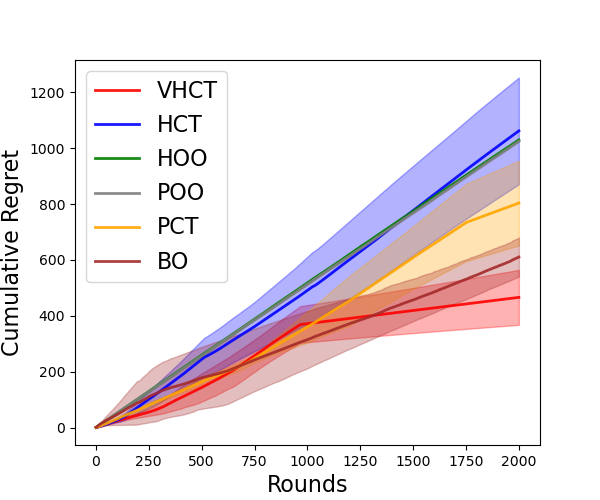
In this section, we empirically compare the proposed VHCT algorithm with the existing anytime blackbox optimization algorithms, including T-HOO (the truncated version of HOO), HCT, POO, and PCT (POO + HCT, (Shang et al., 2019)), and Bayesian Optimization algorithm BO (Frazier, 2018) to validate that the proposed variance-adaptive uncertainty quantifier can make the convergence of VHCT faster than non-adaptive algorithms. We run every algorithm for 20 independent trials in each experiment and plot the average cumulative regret with 1-standard deviation error bounds. The experimental details and additional numerical results on other objectives are provided in Appendix E.

Refer to caption
(a) Garland
Refer to caption
(b) Landmine
Refer to caption
(c) MNIST
Figure 3: Cumulative regret of different algorithms on evaluating the Garland function and tuning hyperparameters of training SVM on Landmine data and neural networks on MNIST data.

We use a noisy Garland function as the synthetic objective, which is a typical blackbox objective used by many works such as Shang et al. (2019) and has multiple local minimums and thus very hard to optimize. For the real-life experiments, we use hyperparameter tuning of machine learning algorithms as the blackbox objectives. We tune the RBF kernel and the L2 regularization parameters when training Support Vector Machine (SVM) on the Landmine dataset (Liu et al., 2007), and the batch size, the learning rate, and the weight decay when training neural networks on the MNIST dataset (Deng, 2012). As shown in Figure 3, the new choice of SE makes VHCT the fastest algorithm among the existing ones. All the experimental results validate our theoretical claims in Section 4.

6 Conclusions

The proposed optimum-statistical collaboration framework reveals and utilizes the fundamental interplay of resolution and uncertainty to design more general and efficient black-box optimization algorithms. Our analysis shows that different regret guarantees can be obtained for functions and partitions with different local smoothness assumptions, and algorithms that have different uncertainty quantifiers. Based on the framework, we show that functions that satisfy the general local smoothness property can be optimized and analyzed, which is a much larger class of functions compared with prior works. Also, we propose a new algorithm VHCT that can adapt to different noises and analyze its performance under different assumptions of the smoothness of the function.

There are still some limitations of our work. For example, VHCT still needs the prior knowledge of the smoothness function ϕ(h)\phi(h) to achieve its best performance. Also, the analyses in Theorem 4.1 and 4.2 are smoothness-specific. Therefore, our framework also introduces many interesting future working directions, for example, (1) whether a unified regret upper bound for different ϕ(h)\phi(h)-local smooth functions could be derived for one particular algorithm; (2) whether the regret bound obtained in Theorem 4.2 is minimax-optimal for those ϕ(h)\phi(h); (3) whether there exists an algorithm that is truly smoothness-agnostic, i.e., it does not need the smoothness property of the objective function.

References

  • Audibert et al. (2006) Jean-Yves Audibert, Remi Munos, and Csaba Szepesvári. Use of variance estimation in the multi-armed bandit problem. 01 2006.
  • Audibert et al. (2009) Jean-Yves Audibert, Rémi Munos, and Csaba Szepesvári. Exploration-exploitation tradeoff using variance estimates in multi-armed bandits. Theoretical Computer Science, 410(19):1876–1902, 2009.
  • Auer et al. (2007) Peter Auer, Ronald Ortner, and Csaba Szepesvári. Improved rates for the stochastic continuum-armed bandit problem. In Nader H. Bshouty and Claudio Gentile, editors, Conference on Learning Theory, pages 454–468, 2007.
  • Azar et al. (2014) Mohammad Gheshlaghi Azar, Alessandro Lazaric, and Emma Brunskill. Online stochastic optimization under correlated bandit feedback. In International Conference on Machine Learning, pages 1557–1565. PMLR, 2014.
  • Bartlett et al. (2019) Peter L. Bartlett, Victor Gabillon, and Michal Valko. A simple parameter-free and adaptive approach to optimization under a minimal local smoothness assumption. In 30th International Conference on Algorithmic Learning Theory, 2019.
  • Bubeck et al. (2011a) Sébastien Bubeck, Rémi Munos, and Gilles Stoltz. Pure exploration in finitely-armed and continuous-armed bandits. Theoretical Computer Science, 412(19):1832–1852, 2011a.
  • Bubeck et al. (2011b) Sébastien Bubeck, Rémi Munos, Gilles Stoltz, and Csaba Szepesvári. X-armed bandits. Journal of Machine Learning Research, 12(46):1655–1695, 2011b.
  • Dai et al. (2020) Zhongxiang Dai, Bryan Kian Hsiang Low, and Patrick Jaillet. Federated bayesian optimization via thompson sampling. In H. Larochelle, M. Ranzato, R. Hadsell, M. F. Balcan, and H. Lin, editors, Advances in Neural Information Processing Systems, volume 33, pages 9687–9699. Curran Associates, Inc., 2020. URL https://proceedings.neurips.cc/paper/2020/file/6dfe08eda761bd321f8a9b239f6f4ec3-Paper.pdf.
  • Deng (2012) Li Deng. The mnist database of handwritten digit images for machine learning research. IEEE Signal Processing Magazine, 29(6):141–142, 2012.
  • Duchi et al. (2015) John C. Duchi, Michael I. Jordan, Martin J. Wainwright, and Andre Wibisono. Optimal rates for zero-order convex optimization: The power of two function evaluations. IEEE Transactions on Information Theory, 61(5):2788–2806, 2015. doi: 10.1109/TIT.2015.2409256.
  • Frazier (2018) Peter I. Frazier. A tutorial on bayesian optimization, 2018. URL https://arxiv.org/abs/1807.02811.
  • Golovin et al. (2017) Daniel Golovin, Benjamin Solnik, Subhodeep Moitra, Greg Kochanski, John Karro, and D Sculley. Google vizier: A service for black-box optimization. In Proceedings of the 23rd ACM SIGKDD international conference on knowledge discovery and data mining, pages 1487–1495, 2017.
  • Grill et al. (2015) Jean-Bastien Grill, Michal Valko, Remi Munos, and Remi Munos. Black-box optimization of noisy functions with unknown smoothness. In Advances in Neural Information Processing Systems. Curran Associates, Inc., 2015.
  • Kandasamy et al. (2018) Kirthevasan Kandasamy, Akshay Krishnamurthy, Jeff Schneider, and Barnabas Poczos. Parallelised bayesian optimisation via thompson sampling. In Amos Storkey and Fernando Perez-Cruz, editors, Proceedings of the Twenty-First International Conference on Artificial Intelligence and Statistics, volume 84 of Proceedings of Machine Learning Research, pages 133–142. PMLR, 09–11 Apr 2018.
  • Kawaguchi et al. (2016) Kenji Kawaguchi, Yu Maruyama, and Xiaoyu Zheng. Global continuous optimization with error bound and fast convergence. Journal of Artificial Intelligence Research, 56:153–195, 2016.
  • Komljenovic et al. (2019) Dragan Komljenovic, Darragi Messaoudi, Alain Cote, Mohamed Gaha, Luc Vouligny, Stephane Alarie, and Olivier Blancke. Asset management in electrical utilities in the context of business and operational complexity. In World Congress on Resilience, Reliability and Asset Management, 07 2019.
  • Li et al. (2018) Lisha Li, Kevin Jamieson, Giulia DeSalvo, Afshin Rostamizadeh, and Ameet Talwalkar. Hyperband: A novel bandit-based approach to hyperparameter optimization. Journal of Machine Learning Research, 18(185):1–52, 2018.
  • Li et al. (2022) Wenjie Li, Qifan Song, Jean Honorio, and Guang Lin. Federated x-armed bandit, 2022. URL https://arxiv.org/abs/2205.15268.
  • Li et al. (2023) Wenjie Li, Haoze Li, Jean Honorio, and Qifan Song. Pyxab – a python library for 𝒳\mathcal{X}-armed bandit and online blackbox optimization algorithms, 2023. URL https://arxiv.org/abs/2303.04030.
  • Liu et al. (2007) Qiuhua Liu, Xuejun Liao, and Lawrence Carin. Semi-supervised multitask learning. In J. Platt, D. Koller, Y. Singer, and S. Roweis, editors, Advances in Neural Information Processing Systems, volume 20. Curran Associates, Inc., 2007. URL https://proceedings.neurips.cc/paper/2007/file/a34bacf839b923770b2c360eefa26748-Paper.pdf.
  • Maillard (2019) Odalric-Ambrym Maillard. Mathematics of statistical sequential decision making. PhD thesis, Université de Lille, Sciences et Technologies, 2019.
  • Maurer and Pontil (2009) Andreas Maurer and Massimiliano Pontil. Empirical bernstein bounds and sample variance penalization. arXiv preprint arXiv:0907.3740, 2009.
  • Munos (2011) Rémi Munos. Optimistic optimization of a deterministic function without the knowledge of its smoothness. In J. Shawe-Taylor, R. Zemel, P. Bartlett, F. Pereira, and K. Q. Weinberger, editors, Advances in Neural Information Processing Systems, volume 24. Curran Associates, Inc., 2011.
  • Shahriari et al. (2016) Bobak Shahriari, Kevin Swersky, Ziyu Wang, Ryan P. Adams, and Nando de Freitas. Taking the human out of the loop: A review of bayesian optimization. Proceedings of the IEEE, 104(1):148–175, 2016.
  • Shamir (2015) Ohad Shamir. An optimal algorithm for bandit and zero-order convex optimization with two-point feedback. Journal of Machine Learning Research, 18, 07 2015.
  • Shang et al. (2019) Xuedong Shang, Emilie Kaufmann, and Michal Valko. General parallel optimization a without metric. In Algorithmic Learning Theory, pages 762–788, 2019.
  • Valko et al. (2013) Michal Valko, Alexandra Carpentier, and Rémi Munos. Stochastic simultaneous optimistic optimization. In Proceedings of the 30th International Conference on Machine Learning, volume 28 of Proceedings of Machine Learning Research, pages 19–27. PMLR, 17–19 Jun 2013.
  • Wang et al. (2020) Chi-Hua Wang, Zhanyu Wang, Will Wei Sun, and Guang Cheng. Online regularization for high-dimensional dynamic pricing algorithms. arXiv preprint arXiv:2007.02470, 2020.
  • Wang et al. (2022) ChiHua Wang, Wenjie Li, Guang Cheng, and Guang Lin. Federated online sparse decision making. ArXiv, abs/2202.13448, 2022.

Appendix A Proof of the General Regret Bound in Theorem 3.1

Proof. We decompose the cumulative regret into two terms that depend on the high probability events {t}t=1n\left\{\mathcal{E}_{t}\right\}_{t=1}^{n}. Denote the simple regret at each iteration tt to be Δt=frt\Delta_{t}=f^{*}-r_{t}, then we can perform the following regret decomposition

Rn\displaystyle R_{n} =t=1nΔt=(t=1nΔt𝕀t)+(t=1nΔt𝕀tc)=Rn+Rnc\displaystyle=\sum_{t=1}^{n}\Delta_{t}=\left(\sum_{t=1}^{n}\Delta_{t}\mathbb{I}_{\mathcal{E}_{t}}\right)+\left(\sum_{t=1}^{n}\Delta_{t}\mathbb{I}_{\mathcal{E}_{t}^{c}}\right)=R_{n}^{\mathcal{E}}+R_{n}^{\mathcal{E}^{c}}
Rn+t=1n𝕀tc\displaystyle\leq R_{n}^{\mathcal{E}}+\sum_{t=1}^{n}\mathbb{I}_{\mathcal{E}_{t}^{c}}

where we have denoted the first summation term in the second equality t=1nΔt𝕀t\sum_{t=1}^{n}\Delta_{t}\mathbb{I}_{\mathcal{E}_{t}} to be RnR_{n}^{\mathcal{E}} and the second summation term t=1nΔt𝕀tc\sum_{t=1}^{n}\Delta_{t}\mathbb{I}_{\mathcal{E}_{t}^{c}} to be RncR_{n}^{\mathcal{E}^{c}}. The last inequality is because we have that both ff^{*} and rtr_{t} are bounded by [0, 1], and thus |Δt|1|\Delta_{t}|\leq 1. Now note that the instantaneous regret Δt\Delta_{t} can be written as

Δt=frt=ff(xht,it)+f(xht,it)rt=Δht,it+Δ^t\Delta_{t}=f^{*}-r_{t}=f^{*}-f\left(x_{h_{t},i_{t}}\right)+f\left(x_{h_{t},i_{t}}\right)-r_{t}=\Delta_{h_{t},i_{t}}+\widehat{\Delta}_{t}

where we have denoted Δht,it=ff(xht,it)\Delta_{h_{t},i_{t}}=f^{*}-f\left(x_{h_{t},i_{t}}\right) and Δ^t=f(xht,it)rt\widehat{\Delta}_{t}=f\left(x_{h_{t},i_{t}}\right)-r_{t}. It means that the regret under the events {t}t=1n\{\mathcal{E}_{t}\}_{t=1}^{n} can be decomposed into two terms R~n\widetilde{R}_{n}^{\mathcal{E}} and R^n\widehat{R}_{n}^{\mathcal{E}}.

Rn=t=1nΔht,it𝕀t+t=1nΔ^t𝕀tt=1nΔht,it𝕀t+t=1nΔ^t=R~n+R^nR_{n}^{\mathcal{E}}=\sum_{t=1}^{n}\Delta_{h_{t},i_{t}}\mathbb{I}_{\mathcal{E}_{t}}+\sum_{t=1}^{n}\widehat{\Delta}_{t}\mathbb{I}_{\mathcal{E}_{t}}\leq\sum_{t=1}^{n}\Delta_{h_{t},i_{t}}\mathbb{I}_{\mathcal{E}_{t}}+\sum_{t=1}^{n}\widehat{\Delta}_{t}=\widetilde{R}_{n}^{\mathcal{E}}+\widehat{R}_{n}^{\mathcal{E}}

Note that by the definition of the sequence {Δ^t}t=1n\{\widehat{\Delta}_{t}\}_{t=1}^{n}, it is a bounded martingale difference sequence since 𝔼[Δ^tt1]=0\mathbb{E}[\widehat{\Delta}_{t}\mid\mathcal{F}_{t-1}]=0 and |Δ^t|1|\widehat{\Delta}_{t}|\leq 1, where t\mathcal{F}_{t} is defined to be the filtration generated up to time tt. Therefore by Azuma’s inequality on this sequence, we get

R^n2nlog(4n2δ)\widehat{R}_{n}^{\mathcal{E}}\leq\sqrt{2n\log\left(\frac{4n^{2}}{\delta}\right)}

with probability 1δ/(4n2)1-\delta/(4n^{2}). A even better bound can be obtained using the fact that |Δ^t|b2|\widehat{\Delta}_{t}|\leq\frac{b}{2} if b2b\ll 2. However, R^n\widehat{R}_{n}^{\mathcal{E}} is not a dominating term and using b/2{b}/{2} only improves it in terms of the multiplicative constant. Now the only term left is R~n\widetilde{R}_{n}^{\mathcal{E}} and we bound it as follows.

R~n\displaystyle\widetilde{R}^{\mathcal{E}}_{n} =(t=1nΔht,it𝕀t)(h=1H(n)i:Th,i(t)0t=1nΔh,i𝕀(ht,it)=(h,i)𝕀t)\displaystyle=\left(\sum_{t=1}^{n}\Delta_{h_{t},i_{t}}\mathbb{I}_{\mathcal{E}_{t}}\right)\leq\left(\sum_{h=1}^{H(n)}\sum_{i:T_{h,i}(t)\neq 0}\sum_{t=1}^{n}\Delta_{h,i}\mathbb{I}_{(h_{t},i_{t})=(h,i)}\mathbb{I}_{\mathcal{E}_{t}}\right)
h=1H¯i:Th,i(t)0t=1na𝚂𝙴h,i(T,t)+H¯+1H(n)i:Th,i(t)0t=1na𝚂𝙴h,i(T,t)\displaystyle\leq\sum_{h=1}^{\overline{H}}\sum_{i:T_{h,i}(t)\neq 0}\sum_{t=1}^{n}a\mathtt{SE}_{h,i}(T,t)+\sum_{\overline{H}+1}^{H(n)}\sum_{i:T_{h,i}(t)\neq 0}\sum_{t=1}^{n}a\mathtt{SE}_{h,i}(T,t)
ah=1H¯i:Th,i(t)0t=1n𝚂𝙴h,i(T,t)(I)+aH¯+1H(n)i:Th,i(t)0t=1n𝚂𝙴h,i(T,t)(II)\displaystyle\leq\underbrace{a\sum_{h=1}^{\overline{H}}\sum_{i:T_{h,i}(t)\neq 0}\sum_{t=1}^{n}\mathtt{SE}_{h,i}(T,t)}_{(\text{I})}+\underbrace{a\sum_{\overline{H}+1}^{H(n)}\sum_{i:T_{h,i}(t)\neq 0}\sum_{t=1}^{n}\mathtt{SE}_{h,i}(T,t)}_{(\text{II})}

where H¯\overline{H} is a constant between 0 and H(n)H(n) to be tuned later. The second inequality is because when we select 𝒫ht,it\mathcal{P}_{h_{t},i_{t}}, we have 𝚂𝙴ht,it(T,t)𝙾𝙴ht\mathtt{SE}_{h_{t},i_{t}}(T,t)\geq\mathtt{OE}_{h_{t}} by the Optimum-statistical Collaboration Framework. Also, under the event t\mathcal{E}_{t}, we have Δht,itamax{𝙾𝙴ht,𝚂𝙴ht,it(T,t)}\Delta_{h_{t},i_{t}}\leq a\max\{\mathtt{OE}_{h_{t}},\mathtt{SE}_{h_{t},i_{t}}(T,t)\}. The first term (I)(\text{I}) can be bounded as

(I)\displaystyle(\text{I}) ah=1H¯i:Th,i(t)0t=1nmaxi:Th,i(t)0𝚂𝙴h,i(T,t)ah=1H¯|h(n)|t=1nmaxi:Th,i(t)0𝚂𝙴h,i(T,t)\displaystyle\leq a\sum_{h=1}^{\overline{H}}\sum_{i:T_{h,i}(t)\neq 0}\sum_{t=1}^{n}\max_{i:T_{h,i}(t)\neq 0}\mathtt{SE}_{h,i}(T,t)\leq a\sum_{h=1}^{\overline{H}}|\mathcal{I}_{h}(n)|\sum_{t=1}^{n}\max_{i:T_{h,i}(t)\neq 0}\mathtt{SE}_{h,i}(T,t)
ah=1H¯2𝒩h1(a𝙾𝙴h1)t=1nmaxi:Th,i(t)0𝚂𝙴h,i(T,t)\displaystyle\leq a\sum_{h=1}^{\overline{H}}2\mathcal{N}_{h-1}\left(a\mathtt{OE}_{h-1}\right)\sum_{t=1}^{n}\max_{i:T_{h,i}(t)\neq 0}\mathtt{SE}_{h,i}(T,t)
2aCh=1H¯(𝙾𝙴h1)d¯t=1nmaxi:Th,i(t)0𝚂𝙴h,i(T,t)\displaystyle\leq 2aC\sum_{h=1}^{\overline{H}}\left(\mathtt{OE}_{h-1}\right)^{-\bar{d}}\sum_{t=1}^{n}\max_{i:T_{h,i}(t)\neq 0}\mathtt{SE}_{h,i}(T,t)

where d¯>d(a,C,𝙾𝙴h1)\bar{d}>d(a,C,\mathtt{OE}_{h-1}) and d(a,C,𝙾𝙴h1)d(a,C,\mathtt{OE}_{h-1}) is the near-optimality dimension with respect to (a,C,𝙾𝙴h1)(a,C,\mathtt{OE}_{h-1}). The third inequality is because we only expand a node into two children, so |h(n)|2|h1+(n)||\mathcal{I}_{h}(n)|\leq 2|\mathcal{I}^{+}_{h-1}(n)| (Note that we do not have any requirements on the number of children of each node, so the binary tree argument here can be easily replaced by a KK-nary tree with K2K\geq 2). Also since we only select a node (h,i)(h,i) when its parent is already selected enough number of times such that 𝙾𝙴𝚂𝙴\mathtt{OE}\geq\mathtt{SE} at a particular time t0nt_{0}\leq n, we have 𝒫hp,ip\mathcal{P}_{{h^{p},i^{p}}} satisfies ff(xhp,ip)a𝙾𝙴hpf^{*}-f(x_{h^{p},i^{p}})\leq a\mathtt{OE}_{h^{p}}. By the definition of 𝒩h(ϵ)\mathcal{N}_{h}(\epsilon) in the near-optimality dimension, we have

|h(n)|2|h1+(n)|2𝒩h1(a𝙾𝙴h1)\displaystyle|\mathcal{I}_{h}(n)|\leq 2|\mathcal{I}^{+}_{h-1}(n)|\leq 2\mathcal{N}_{h-1}\left(a\mathtt{OE}_{h-1}\right)

and thus the final upper bound for (I)(\text{I}). Therefore for any H¯[1,H(n)]\overline{H}\in[1,H(n)], with probability at least 1δ4n21-\frac{\delta}{4n^{2}}, the cumulative regret is upper bounded by

Rn\displaystyle R_{n} =t=1nΔt=R^n+t=1n𝕀(tc)+R~n\displaystyle=\sum_{t=1}^{n}\Delta_{t}=\widehat{R}_{n}^{\mathcal{E}}+\sum_{t=1}^{n}\mathbb{I}({\mathcal{E}_{t}^{c}})+\widetilde{R}_{n}^{\mathcal{E}}
2nlog(4n2/δ)+t=1n𝕀(tc)+R~n\displaystyle\leq\sqrt{2n\log({4n^{2}/\delta})}+\sum_{t=1}^{n}\mathbb{I}({\mathcal{E}_{t}^{c}})+\widetilde{R}^{\mathcal{E}}_{n}
2nlog(4n2/δ)+t=1n𝕀(tc)+2aCh=1H¯(𝙾𝙴h1)d¯t=1nmaxi:Th,i(t)0𝚂𝙴h,i(T,t)\displaystyle\leq\sqrt{2n\log({4n^{2}/\delta})}+\sum_{t=1}^{n}\mathbb{I}({\mathcal{E}_{t}^{c}})+2aC\sum_{h=1}^{\overline{H}}\left(\mathtt{OE}_{h-1}\right)^{-\bar{d}}\sum_{t=1}^{n}\max_{i:T_{h,i}(t)\neq 0}\mathtt{SE}_{h,i}(T,t)
+aH¯+1H(n)i:Th,i(t)0t=1n𝚂𝙴h,i(T,t)\displaystyle\quad+{a\sum_{\overline{H}+1}^{H(n)}\sum_{i:T_{h,i}(t)\neq 0}\sum_{t=1}^{n}\mathtt{SE}_{h,i}(T,t)}

\square

Appendix B Notations and Useful Lemmas

B.1 Preliminary Notations

The notations here follow those in Shang et al. [2019] and Azar et al. [2014] except for those related to the node variance. These notations are needed for the proof of the main theorem.

  • At each time tt, 𝒫ht,it\mathcal{P}_{h_{t},i_{t}} denote the node selected by the algorithm where hth_{t} is the level and iti_{t} is the index.

  • PtP_{t} denotes the optimal-path selected at each iteration tt

  • H(t)H(t) denotes the maximum depth of the tree at time tt.

  • Δ(t)=1/δ~(t+)\Delta(t)=1/\tilde{\delta}(t^{+}) with t+=2logt+1t^{+}=2^{\lfloor\log t\rfloor+1}, δ~(t)=min{1,c1δ/t}\tilde{\delta}(t)=\min\{1,c_{1}\delta/t\}

  • For any t>0t>0 and h[1,H(t)]h\in[1,H(t)], h(t)\mathcal{I}_{h}(t) denotes the set of all nodes at level hh at time tt.

  • For any t>0t>0 and h[1,H(t)]h\in[1,H(t)], h+(t)\mathcal{I}^{+}_{h}(t) denotes the subset of h(t)\mathcal{I}_{h}(t) that contains only the internal nodes (no leaves).

  • 𝒞h,i:={t[1,n]𝒫ht,it=𝒫h,i}\mathcal{C}_{h,i}:=\left\{t\in[1,n]\mid\mathcal{P}_{h_{t},i_{t}}=\mathcal{P}_{h,i}\right\} is the set of time steps when 𝒫h,i\mathcal{P}_{h,i} is selected.

  • 𝒞h,i+:=𝒞h+1,2i𝒞h+1,2i1\mathcal{C}^{+}_{h,i}:=\mathcal{C}_{h+1,2i}\cup\mathcal{C}_{h+1,2i-1} is the set of time steps when the children of 𝒫h,i\mathcal{P}_{h,i} are selected.

  • t¯h,i:=maxt𝒞h,it\bar{t}_{h,i}:=\max_{t\in\mathcal{C}_{h,i}}t is the last time 𝒫h,i\mathcal{P}_{h,i} is selected.

  • t~h,i:=maxt𝒞h,i+t\widetilde{t}_{h,i}:=\max_{t\in\mathcal{C}^{+}_{h,i}}t is the last time when the children of 𝒫h,i\mathcal{P}_{h,i} is selected.

  • th,i:=min{t:Th,i(t)τh,i}{t}_{h,i}:=\min\left\{t:T_{h,i}(t)\geq\tau_{h,i}\right\} is the time when 𝒫h,i\mathcal{P}_{h,i} is expanded.

  • 𝕍^h,i(t):=1Th,i(t)s=1Th,i(t)(rs(xh,i)μ^h,i)\widehat{\mathbb{V}}_{h,i}(t):=\frac{1}{T_{h,i}(t)}\sum_{s=1}^{T_{h,i}(t)}\left(r^{s}(x_{h,i})-\widehat{\mu}_{h,i}\right) is the estimate of the variance of the 𝒫h,i\mathcal{P}_{h,i} node at time tt.

  • t\mathcal{L}_{t} denotes all the nodes in the exploration tree at time tt

  • VmaxV_{\max} is the upper bound on the node variance in the tree.

Note that if the variance of a node is zero, we can always pull one more round to make it non-zero. Therefore, here we simply assume that the variance 𝕍h,i(t)\mathbb{V}_{h,i}(t) is larger than a fixed small constant ϵ\epsilon for the clarity of proof, which will not affect our conclusions.

Algorithm 3 VHCT Algorithm (Complete)
1:  Input: Smoothness function ϕ(h)\phi(h), partition 𝒫\mathcal{P}.
2:  Initialize: 𝒯t={𝒫0,1,𝒫1,1,𝒫1,2},U1,1(t)=U1,2(t)=+\mathcal{T}_{t}=\{\mathcal{P}_{0,1},\mathcal{P}_{1,1},\mathcal{P}_{1,2}\},U_{1,1}(t)=U_{1,2}(t)=+\infty
3:  for t=1t=1 to nn do
4:     if t=t+t=t^{+} then
5:        for all nodes 𝒫h,i𝒯t\mathcal{P}_{h,i}\in\mathcal{T}_{t}  do
6:           Uh,i(t)=μh,i(t)+ϕ(h)+𝚂𝙴h,i(T,t)U_{h,i}(t)=\mu_{h,i}(t)+\phi(h)+\mathtt{SE}_{h,i}(T,t)
7:        end for
8:        𝚄𝚙𝚍𝚊𝚝𝚎𝙱𝚊𝚌𝚔𝚠𝚊𝚛𝚍(𝒯t,t)\mathtt{UpdateBackward}(\mathcal{T}_{t},t)
9:     end if
10:     𝒫ht,it=𝙿𝚞𝚕𝚕𝚄𝚙𝚍𝚊𝚝𝚎(𝒯t,t)\mathcal{P}_{h_{t},i_{t}}=\mathtt{PullUpdate}(\mathcal{T}_{t},t)
11:     if Tht,it(t)τht,it(t)T_{h_{t},i_{t}}(t)\geq\tau_{h_{t},i_{t}}(t) and 𝒫ht,it\mathcal{P}_{h_{t},i_{t}} is a leaf then
12:        𝒯t=𝒯t{𝒫ht+1,2it1,𝒫ht+1,2it}\mathcal{T}_{t}=\mathcal{T}_{t}\cup\{\mathcal{P}_{h_{t}+1,2i_{t}-1},\mathcal{P}_{h_{t}+1,2i_{t}}\}
13:        Uh+1,2i(t)=Uh+1,2i1(t)=+U_{h+1,2i}(t)=U_{h+1,2i-1}(t)=+\infty
14:     end if
15:  end for

Algorithm 4 𝙿𝚞𝚕𝚕𝚄𝚙𝚍𝚊𝚝𝚎\mathtt{PullUpdate}
1:  Input: a tree 𝒯t\mathcal{T}_{t}, round tt
2:  Initialize: (ht,it)=(0,1);St=𝒫0,1;T0,1(t)=τ0(t)=1(h_{t},i_{t})=(0,1);S_{t}=\mathcal{P}_{0,1};T_{0,1}(t)=\tau_{0}(t)=1 ;
3:  while  𝒫ht,it\mathcal{P}_{h_{t},i_{t}} is not a leaf, Tht,it(t)τht,it(t)T_{h_{t},i_{t}}(t)\geq\tau_{h_{t},i_{t}}(t) do
4:     j=argmaxj=0,1{Bht+1,2itj(t)}j=\text{argmax}_{j=0,1}\{B_{h_{t}+1,2i_{t}-j}(t)\}
5:     (ht,it)=(ht+1,2itj)(h_{t},i_{t})=(h_{t}+1,2i_{t}-j)
6:     St=St{𝒫ht,it}S_{t}=S_{t}\cup\{\mathcal{P}_{h_{t},i_{t}}\}
7:  end while
8:  Pull xht,itx_{h_{t},i_{t}} and get reward rtr_{t}
9:  Tht,it(t)=Tht,it(t)+1T_{h_{t},i_{t}}(t)=T_{h_{t},i_{t}}(t)+1
10:  Update μ^ht,it(t)\widehat{\mu}_{h_{t},i_{t}}(t), 𝕍^ht,it(t)\widehat{\mathbb{V}}_{h_{t},i_{t}}(t)
11:  Uht,it(t)=μ^ht,it(t)+ϕ(ht)+𝚂𝙴ht,it(T,t)U_{h_{t},i_{t}}(t)=\widehat{\mu}_{h_{t},i_{t}}(t)+\phi(h_{t})+\mathtt{SE}_{h_{t},i_{t}}(T,t)
12:  𝚄𝚙𝚍𝚊𝚝𝚎𝙱𝚊𝚌𝚔𝚠𝚊𝚛𝚍(St,t)\mathtt{UpdateBackward}(S_{t},t)
13:  Return 𝒫ht,it\mathcal{P}_{h_{t},i_{t}}
Algorithm 5 𝚄𝚙𝚍𝚊𝚝𝚎𝙱𝚊𝚌𝚔𝚠𝚊𝚛𝚍\mathtt{UpdateBackward}
1:  Input: a tree 𝒯\mathcal{T}, round tt
2:  for  𝒫h,i𝒯\mathcal{P}_{h,i}\in\mathcal{T} backward from each leaf of 𝒯\mathcal{T} do
3:     if  𝒫h,i\mathcal{P}_{h,i} is a leaf of 𝒯\mathcal{T} then
4:        Bh,i(t)=Uh,i(t)B_{h,i}(t)=U_{h,i}(t)
5:     else
6:        Bh,i(t)=min{Uh,i(t),maxj{Bh+1,2ij(t)}}B_{h,i}(t)=\min\left\{U_{h,i}(t),\max_{j}\{B_{h+1,2i-j}(t)\}\right\}
7:     end if
8:     Update the threshold τh,i(t)\tau_{h,i}(t)
9:  end for

B.2 Useful Lemmas for the Proof of Theorem 4.1 and Theorem 4.2

The following lemma improves the results by Azar et al. [2014] and Shang et al. [2019].

Lemma B.1.

We introduce the following event t\mathcal{E}_{t}

t={𝒫h,it,Th,i(t)=1,,t:|μ^h,i(t)f(xh,i)|c2𝕍^h,i(t)log(1/δ~(t))Th,i(t)+3bc2log(1/δ~(t))Th,i(t)}\mathcal{E}_{t}=\left\{\forall\mathcal{P}_{h,i}\in\mathcal{L}_{t},\forall T_{h,i}(t)=1,\cdots,t:\left|\widehat{\mu}_{h,i}(t)-f\left(x_{h,i}\right)\right|\leq c\sqrt{\frac{2\widehat{\mathbb{V}}_{h,i}(t)\log(1/\tilde{\delta}(t))}{T_{h,i}(t)}}+\frac{3bc^{2}\log(1/\tilde{\delta}(t))}{T_{h,i}(t)}\right\}

where xh,i𝒫h,ix_{h,i}\in\mathcal{P}_{h,i} is the arm corresponding to node 𝒫h,i.\mathcal{P}_{h,i}. If

c=3 and δ~(t)=δ3tc=3\quad\text{ and }\quad\tilde{\delta}(t)=\frac{\delta}{3t}

then for any fixed t, the event t\mathcal{E}_{t} holds with probability at least 1δ/t71-\delta/t^{7}.

Proof. Again, t\mathcal{L}_{t} denotes all the nodes in the tree. The probability of tc\mathcal{E}_{t}^{c} can be bounded as

[tc]\displaystyle\mathbb{P}\bigg{[}\mathcal{E}_{t}^{\mathrm{c}}\bigg{]} 𝒫h,itTh,i(t)=1t[|μ^h,i(t)μh,i|c2𝕍^h,i(t)log(1/δ~(t))Th,i(t)+3bc2log(1/δ~(t))Th,i(t)]\displaystyle\leq\sum_{\mathcal{P}_{h,i}\in\mathcal{L}_{t}}\sum_{T_{h,i}(t)=1}^{t}\mathbb{P}\bigg{[}\left|\widehat{\mu}_{h,i}(t)-\mu_{h,i}\right|\geq c\sqrt{\frac{2\widehat{\mathbb{V}}_{h,i}(t)\log(1/\tilde{\delta}(t))}{T_{h,i}(t)}}+\frac{3bc^{2}\log(1/\tilde{\delta}(t))}{T_{h,i}(t)}\bigg{]}
𝒫h,itTh,i(t)=1t3exp(c2log(1/δ~(t)))\displaystyle\leq\sum_{\mathcal{P}_{h,i}\in\mathcal{L}_{t}}\sum_{T_{h,i}(t)=1}^{t}3\exp(-c^{2}\log(1/\tilde{\delta}(t)))
=3exp(c2log(1/δ~(t)))t|t|\displaystyle=3\exp(-c^{2}\log(1/\tilde{\delta}(t)))\cdot t\cdot\left|\mathcal{L}_{t}\right|

where the second inequality is by taking x=c2log(1/δ~(t))x=c^{2}\log(1/\tilde{\delta}(t)) in Lemma B.6, we have

(|μ^h,i(t)f(xh,i)|c2𝕍^h,i(t)log(1/δ~(t))Th,i(t)+3bc2log(1/δ~(t))Th,i(t))3exp(c2log(1/δ~(t)))\displaystyle\mathbb{P}\bigg{(}|\widehat{\mu}_{h,i}(t)-f\left(x_{h,i}\right)|\geq c\sqrt{\frac{2\widehat{\mathbb{V}}_{h,i}(t)\log(1/\tilde{\delta}(t))}{T_{h,i}(t)}}+\frac{3bc^{2}\log(1/\tilde{\delta}(t))}{T_{h,i}(t)}\bigg{)}\leq 3\exp(-c^{2}\log(1/\tilde{\delta}(t)))

Now note that the number of nodes in the tree is always (loosely) bounded by tt since we need at least one pull to expand a node, we know that

[tc]\displaystyle\mathbb{P}\bigg{[}\mathcal{E}_{t}^{\mathrm{c}}\bigg{]} 3t2δ~(t)c2δt7\displaystyle\leq 3t^{2}\tilde{\delta}(t)^{c^{2}}\leq\frac{\delta}{t^{7}} \square
Lemma B.2.

Given the parameters cc and δ~(t)\tilde{\delta}(t) as in Lemma B.1, the regret when the events {t}\{\mathcal{E}_{t}\} fail to hold is bounded as

t=1n𝕀(tc)n\sum_{t=1}^{n}\mathbb{I}({\mathcal{E}_{t}^{c}})\leq\sqrt{n}

with probability at least 1δ/(6n3)1-\delta/(6n^{3})

Proof. We first split the time horizon nn in two phases: the first phase until n\sqrt{n} and the rest. Thus the regret bound becomes

t=1n𝕀(tc)=t=1n𝕀(tc)+t=n+1n𝕀(tc)\sum_{t=1}^{n}\mathbb{I}({\mathcal{E}_{t}^{c}})=\sum_{t=1}^{\sqrt{n}}\mathbb{I}({\mathcal{E}_{t}^{c}})+\sum_{t=\sqrt{n}+1}^{n}\mathbb{I}({\mathcal{E}_{t}^{c}})

The first term can be easily bounded by n\sqrt{n}. Now we bound the second term by showing that the complement of the high-probability event hardly ever happens after t=nt=\sqrt{n}. By Lemma B.1

[t=n+1ntc]t=n+1n[tc]n+1nδt7n+δt7𝑑tδ6n3\mathbb{P}\left[\bigcup_{t=\sqrt{n}+1}^{n}\mathcal{E}_{t}^{\mathrm{c}}\right]\leq\sum_{t=\sqrt{n}+1}^{n}\mathbb{P}\left[\mathcal{E}_{t}^{\mathrm{c}}\right]\leq\sum_{\sqrt{n}+1}^{n}\frac{\delta}{t^{7}}\leq\int_{\sqrt{n}}^{+\infty}\frac{\delta}{t^{7}}dt\leq\frac{\delta}{6n^{3}}

Therefore we arrive to the conclusion in the lemma. \square

Lemma B.3.

At time tt under the event t\mathcal{E}_{t}, for the selected node 𝒫ht,it\mathcal{P}_{h_{t},i_{t}} and its parent (htp,itp)(h_{t}^{p},i_{t}^{p}), we have the following set of inequalities for any choice of the local smoothness function ϕ(h)\phi(h) in Algorithm 3

{ff(xht,it)3c2𝕍^ht,it(t)log(2/δ~(t))Tht,it(t)+9bc2log(2/δ~(t))Tht,it(t)ff(xhtp,itp)3ϕ(htp)\left\{\begin{aligned} &f^{*}-f(x_{h_{t},i_{t}})\leq 3c\sqrt{\frac{2\widehat{\mathbb{V}}_{h_{t},i_{t}}(t)\log(2/\tilde{\delta}(t))}{T_{h_{t},i_{t}}(t)}}+\frac{9bc^{2}\log(2/\tilde{\delta}(t))}{T_{h_{t},i_{t}}(t)}\\ \\ &f^{*}-f(x_{h_{t}^{p},i_{t}^{p}})\leq 3\phi(h_{t}^{p})\end{aligned}\right.

Proof. Recall that PtP_{t} is the optimal path traversed. Let (h,i)Pt(h^{\prime},i^{\prime})\in P_{t} and (h′′,i′′)(h^{\prime\prime},i^{\prime\prime}) be the node which immediately follows (h,i)(h{{}^{\prime}},i{{}^{\prime}}) in PtP_{t} (i.e., h=′′h+1)h{{}^{\prime\prime}}=h{{}^{\prime}}+1). By the definition of BB values, we have the following inequality

Bh,i(t)max(Bh+1,2i1(t);Bh+1,2i(t))=Bh′′,i′′(t)B_{h^{\prime},i^{\prime}}(t)\leq\max\left(B_{h^{\prime}+1,2i^{\prime}-1}(t);B_{h^{\prime}+1,2i^{\prime}}(t)\right)=B_{h^{\prime\prime},i^{\prime\prime}}(t)

where the last equality is from the fact that the algorithm selects the child with the larger BB value. By iterating along the inequality until the selected node (ht,it)\left(h_{t},i_{t}\right) and its parent (htp,itp)\left(h_{t}^{p},i_{t}^{p}\right) we obtain

(h,i)Pt,\displaystyle\forall\left(h^{\prime},i^{\prime}\right)\in P_{t}, Bh,i(t)Bht,it(t)Uht,it(t),\displaystyle B_{h^{\prime},i^{\prime}}(t)\leq B_{h_{t},i_{t}}(t)\leq U_{h_{t},i_{t}}(t),
(h,i)Pt(ht,it),\displaystyle\forall\left(h^{\prime},i^{\prime}\right)\in P_{t}-\left(h_{t},i_{t}\right), Bh,i(t)Bhtp,itp(t)Uhtp,itp(t),\displaystyle B_{h^{\prime},i^{\prime}}(t)\leq B_{h_{t}^{p},i_{t}^{p}}(t)\leq U_{h_{t}^{p},i_{t}^{p}}(t),

Thus for any node 𝒫h,iPt,\mathcal{P}_{h,i}\in P_{t}, we have that Uht,it(t)Bh,i(t).U_{h_{t},i_{t}}(t)\geq B_{h,i}(t). Furthermore, since the root node (0,1)(0,1) is a an optimal node in the path PtP_{t}. Therefore, there exists at least one node (h,i)Pt\left(h^{*},i^{*}\right)\in P_{t} which includes the maximizer xx^{*} and has the the depth hhtp<hth^{*}\leq h_{t}^{p}<h_{t}. Thus

Uht,it(t)Bh,i(t),Uhtp,itp(t)Bh,i(t)\displaystyle U_{h_{t},i_{t}}(t)\geq B_{h^{*},i^{*}}(t),\quad U_{h_{t}^{p},i_{t}^{p}}(t)\geq B_{h^{*},i^{*}}(t)

Note that by the definition of Uht,it(t)U_{h_{t},i_{t}}(t), under event t\mathcal{E}_{t}

Uht,it(t)\displaystyle U_{h_{t},i_{t}}(t) =μ^ht,it(t)+ϕ(ht)+c2𝕍^ht,it(t)log(1/δ~(t+))Tht,it(t)+3bc2log(1/δ~(t+))Tht,it(t)\displaystyle=\widehat{\mu}_{h_{t},i_{t}}(t)+\phi(h_{t})+c\sqrt{\frac{2\widehat{\mathbb{V}}_{h_{t},i_{t}}(t)\log(1/\tilde{\delta}(t^{+}))}{T_{h_{t},i_{t}}(t)}}+\frac{3bc^{2}\log(1/\tilde{\delta}(t^{+}))}{T_{h_{t},i_{t}}(t)} (5)
f(xht,it)+ϕ(ht)+c2𝕍^ht,it(t)log(1/δ~(t+))Tht,it(t)+3bc2log(1/δ~(t+))Tht,it(t)\displaystyle\leq f(x_{h_{t},i_{t}})+\phi(h_{t})+c\sqrt{\frac{2\widehat{\mathbb{V}}_{h_{t},i_{t}}(t)\log(1/\tilde{\delta}(t^{+}))}{T_{h_{t},i_{t}}(t)}}+\frac{3bc^{2}\log(1/\tilde{\delta}(t^{+}))}{T_{h_{t},i_{t}}(t)}
+c2𝕍^ht,it(t)log(1/δ~(t))Tht,it(t)+3bc2log(1/δ~(t))Tht,it(t)\displaystyle~{}\qquad+c\sqrt{\frac{2\widehat{\mathbb{V}}_{h_{t},i_{t}}(t)\log(1/\tilde{\delta}(t))}{T_{h_{t},i_{t}}(t)}}+\frac{3bc^{2}\log(1/\tilde{\delta}(t))}{T_{h_{t},i_{t}}(t)}
f(xht,it)+ϕ(ht)+2c2𝕍^ht,it(t)log(1/δ~(t+))Tht,it(t)+6bc2log(1/δ~(t+))Tht,it(t)\displaystyle\leq f(x_{h_{t},i_{t}})+\phi(h_{t})+2c\sqrt{\frac{2\widehat{\mathbb{V}}_{h_{t},i_{t}}(t)\log(1/\tilde{\delta}(t^{+}))}{T_{h_{t},i_{t}}(t)}}+\frac{6bc^{2}\log(1/\tilde{\delta}(t^{+}))}{T_{h_{t},i_{t}}(t)}

where the first inequality holds by the definition of UU and the second one holds by t+tt^{+}\geq t. Similarly the parent node satisfies the above inequality

Uhtp,itp(t)\displaystyle U_{h_{t}^{p},i_{t}^{p}}(t) f(xhtp,itp)+ϕ(htp)+2c2𝕍^htp,itp(t)log(1/δ~(t+))Thtp,itp(t)+6bc2log(1/δ~(t+))Thtp,itp(t)\displaystyle\leq f(x_{h_{t}^{p},i_{t}^{p}})+\phi(h_{t}^{p})+2c\sqrt{\frac{2\widehat{\mathbb{V}}_{h_{t}^{p},i_{t}^{p}}(t)\log(1/\tilde{\delta}(t^{+}))}{T_{h_{t}^{p},i_{t}^{p}}(t)}}+\frac{6bc^{2}\log(1/\tilde{\delta}(t^{+}))}{T_{h_{t}^{p},i_{t}^{p}}(t)}

By Lemma B.4, we know Uh,i(t)fU_{h^{*},i^{*}}(t)\geq f^{*}. If (h,i)(h^{*},i^{*}) is a leaf, then by our definition Bh,i(t)=Uh,i(t)fB_{h^{*},i^{*}}(t)=U_{h^{*},i^{*}}(t)\geq f^{*}. Otherwise, there exists a leaf (hx,ix)(h_{x},i_{x}) containing the maximum point which has (h,i)(h^{*},i^{*}) as its ancestor. Therefore we know that fBhx,ixBh,if^{*}\leq B_{h_{x},i_{x}}\leq B_{h^{*},i^{*}}, so Bh,iB_{h^{*},i^{*}} is always an upper bound for ff^{*}. Now we know that

Δht,it(t)\displaystyle\Delta_{h_{t},i_{t}}(t) :=ff(xht,it)ϕ(ht)+2c2𝕍^ht,it(t)log(1/δ~(t+))Tht,it(t)+6bc2log(1/δ~(t+))Tht,it(t)\displaystyle:=f^{*}-f(x_{h_{t},i_{t}})\leq\phi(h_{t})+2c\sqrt{\frac{2\widehat{\mathbb{V}}_{h_{t},i_{t}}(t)\log(1/\tilde{\delta}(t^{+}))}{T_{h_{t},i_{t}}(t)}}+\frac{6bc^{2}\log(1/\tilde{\delta}(t^{+}))}{T_{h_{t},i_{t}}(t)}
Δhtp,itp(t)\displaystyle\Delta_{h_{t}^{p},i_{t}^{p}}(t) :=ff(xhtp,itp)ϕ(htp)+2c2𝕍^htp,itp(t)log(1/δ~(t+))Thtp,itp(t)+6bc2log(1/δ~(t+))Thtp,itp(t)\displaystyle:=f^{*}-f(x_{h_{t}^{p},i_{t}^{p}})\leq\phi(h_{t}^{p})+2c\sqrt{\frac{2\widehat{\mathbb{V}}_{h_{t}^{p},i_{t}^{p}}(t)\log(1/\tilde{\delta}(t^{+}))}{T_{h_{t}^{p},i_{t}^{p}}(t)}}+\frac{6bc^{2}\log(1/\tilde{\delta}(t^{+}))}{T_{h_{t}^{p},i_{t}^{p}}(t)}

Recall that the algorithm selects a node only when Tht,it(t)<τht,it(t)T_{h_{t},i_{t}}(t)<\tau_{h_{t},i_{t}}(t) and thus the statistical uncertainty is large, i.e., ϕ(ht)𝚂𝙴ht,it(T,t)\phi(h_{t})\leq\mathtt{SE}_{h_{t},i_{t}}(T,t), and the choice of τht,it(t)\tau_{h_{t},i_{t}}(t), we get

Δht,it(t)\displaystyle\Delta_{h_{t},i_{t}}(t) 3c2𝕍^ht,it(t)log(1/δ~(t+))Tht,it(t)+9bc2log(1/δ~(t+))Tht,it(t)\displaystyle\leq 3c\sqrt{\frac{2\widehat{\mathbb{V}}_{h_{t},i_{t}}(t)\log(1/\tilde{\delta}(t^{+}))}{T_{h_{t},i_{t}}(t)}}+\frac{9bc^{2}\log(1/\tilde{\delta}(t^{+}))}{T_{h_{t},i_{t}}(t)}
3c2𝕍^ht,it(t)log(2/δ~(t))Tht,it(t)+9bc2log(2/δ~(t))Tht,it(t)\displaystyle\leq 3c\sqrt{\frac{2\widehat{\mathbb{V}}_{h_{t},i_{t}}(t)\log(2/\tilde{\delta}(t))}{T_{h_{t},i_{t}}(t)}}+\frac{9bc^{2}\log(2/\tilde{\delta}(t))}{T_{h_{t},i_{t}}(t)}

where we used the fact t+2tt^{+}\leq 2t for any tt. For the parent (htp,itp)(h_{t}^{p},i_{t}^{p}), since Thtp,itp(t)τhtp,itp(t)T_{h_{t}^{p},i_{t}^{p}}(t)\geq\tau_{h_{t}^{p},i_{t}^{p}}(t) and thus ϕ(htp)𝚂𝙴htp,itp(T,t)\phi(h_{t}^{p})\geq\mathtt{SE}_{h_{t}^{p},i_{t}^{p}}(T,t), we know that

Δhtp,itp(t)ϕ(htp)+2c2𝕍^htp,itp(t)log(1/δ~(t+))τhtp,itp(t)+6bc2log(1/δ~(t+))τhtp,itp(t)3ϕ(htp)\displaystyle\Delta_{h_{t}^{p},i_{t}^{p}}(t)\leq\phi(h_{t}^{p})+2c\sqrt{\frac{2\widehat{\mathbb{V}}_{h_{t}^{p},i_{t}^{p}}(t)\log(1/\tilde{\delta}(t^{+}))}{\tau_{h_{t}^{p},i_{t}^{p}}(t)}}+\frac{6bc^{2}\log(1/\tilde{\delta}(t^{+}))}{\tau_{h_{t}^{p},i_{t}^{p}}(t)}\leq 3\phi(h_{t}^{p})

The above inequality implies that the selected node 𝒫ht,it\mathcal{P}_{h_{t},i_{t}} must have a 3ϕ(htp)3\phi(h_{t}^{p}) optimal parent under t\mathcal{E}_{t}. \square

Lemma B.4.

(UU Upper Bounds ff^{*}) Under event t\mathcal{E}_{t}, we have that for any optimal node (h,i)\left(h^{*},i^{\star}\right) and any choice of the smoothness function ϕ(h)\phi(h) in Algorithm 3, Uh,i(t)U_{h^{*},i^{*}}(t) is an upper bound on ff^{\star}

Proof. The proof here is similar to that of Lemma 5 in Shang et al. [2019]. Since t+t,t^{+}\geq t, we have

Uh,i(t)\displaystyle U_{h^{*},i^{*}}(t) =μ^h,i(t)+ϕ(h)+c2𝕍^h,i(t)log(1/δ~(t+))Th,i(t)+3bc2log(1/δ~(t+))Th,i(t)\displaystyle=\widehat{\mu}_{h^{*},i^{*}}(t)+\phi(h^{*})+c\sqrt{\frac{2\widehat{\mathbb{V}}_{h^{*},i^{*}}(t)\log(1/\tilde{\delta}(t^{+}))}{T_{h^{*},i^{*}}(t)}}+\frac{3bc^{2}\log(1/\tilde{\delta}(t^{+}))}{T_{h^{*},i^{*}}(t)}
μ^h,i(t)+ϕ(h)+c2𝕍^h,i(t)log(1/δ~(t))Th,i(t)+3bc2log(1/δ~(t))Th,i(t)\displaystyle\geq\widehat{\mu}_{h^{*},i^{*}}(t)+\phi(h^{*})+c\sqrt{\frac{2\widehat{\mathbb{V}}_{h^{*},i^{*}}(t)\log(1/\tilde{\delta}(t))}{T_{h^{*},i^{*}}(t)}}+\frac{3bc^{2}\log(1/\tilde{\delta}(t))}{T_{h^{*},i^{*}}(t)}
ϕ(h)+f(xh,i)\displaystyle\geq\phi(h^{*})+f(x_{h^{*},i^{*}})

where the last inequality is by the event t\mathcal{E}_{t},

μ^h,i(t)+c2𝕍^h,i(t)log(1/δ~(t))Th,i(t)+3bc2log(1/δ~(t))Th,i(t)f(xh,i)\widehat{\mu}_{h^{*},i^{*}}(t)+c\sqrt{\frac{2\widehat{\mathbb{V}}_{h^{*},i^{*}}(t)\log(1/\tilde{\delta}(t))}{T_{h^{*},i^{*}}(t)}}+\frac{3bc^{2}\log(1/\tilde{\delta}(t))}{T_{h^{*},i^{*}}(t)}\geq f(x_{h^{*},i^{*}}) \square
Lemma B.5.

(Details for Solving τ\tau) For any choice of ϕ(h)\phi(h), the solution τh,i(t)\tau_{h,i}(t) to the equation ϕ(h)=𝚂𝙴h,i(T,t)\phi(h)=\mathtt{SE}_{h,i}(T,t) for the proposed VHCT algorithm in Section 4 is

τh,i(t)=(1+1+3bϕ(h)𝕍^h,i(t)/2)2c22ϕ(h)2𝕍^h,i(t)log(1/δ~(t+))\tau_{h,i}(t)=\bigg{(}1+\sqrt{1+\frac{3b\phi(h)}{\widehat{\mathbb{V}}_{h,i}(t)/2}}\bigg{)}^{2}\frac{c^{2}}{2\phi(h)^{2}}\widehat{\mathbb{V}}_{h,i}(t)\log(1/\tilde{\delta}(t^{+})) (6)

Proof. First, we define the following variables for ease of notatioins

{A:=ϕ(h)B:=c2𝕍^h,i(t)log(1/δ~(t+))C:=3bc2log(1/δ~(t+))\left\{\begin{aligned} A&:=\phi(h)\\ B&:=c\sqrt{2\widehat{\mathbb{V}}_{h,i}(t)\log(1/\tilde{\delta}(t^{+}))}\\ C&:=3bc^{2}\log(1/\tilde{\delta}(t^{+}))\end{aligned}\right.

Therefore the original equation ϕ(h)=𝚂𝙴h,i(T,t)\phi(h)=\mathtt{SE}_{h,i}(T,t) can be written as,

A=B1τh,i(t)+Cτh,i(t)\displaystyle A=B\cdot\frac{1}{\sqrt{\tau_{h,i}(t)}}+\frac{C}{\tau_{h,i}(t)}

Note that the above is a quadratic equation of τh,i(t)\tau_{h,i}(t), therefore we arrive at the solution

τh,i(t)\displaystyle\tau_{h,i}(t) =(1+1+3bA𝕍^h,i(t)/2)2c22A2𝕍^h,i(t)log(1/δ~(t+))\displaystyle=\bigg{(}1+\sqrt{1+\frac{3bA}{\widehat{\mathbb{V}}_{h,i}(t)/2}}\bigg{)}^{2}\frac{c^{2}}{2A^{2}}\widehat{\mathbb{V}}_{h,i}(t)\log(1/\tilde{\delta}(t^{+})) \square

B.3 Supporting Lemmas

Lemma B.6.

Let X1,,XtX_{1},\ldots,X_{t} be i.i.d. random variables taking their values in [μb2,μ+b2][\mu-\frac{b}{2},\mu+\frac{b}{2}], where μ=𝔼[Xi]\mu=\mathbb{E}[X_{i}]. Let X¯t,Vt\bar{X}_{t},V_{t} be the mean and variance of {Xi}i=1:t\{X_{i}\}_{i=1:t}. For any tt\in\mathbb{N} and x>0,x>0, with probability at least 13ex1-3e^{-x}, we have

|X¯tμ|2Vtxt+3bxt\left|\bar{X}_{t}-\mu\right|\leq\sqrt{\frac{2V_{t}x}{t}}+\frac{3bx}{t}

Proof. This lemma follows the results in Lemma B.7. Note that X1,X2,,Xt[μb2,μ+b2]X_{1},X_{2},\ldots,X_{t}\in[\mu-\frac{b}{2},\mu+\frac{b}{2}], we can define Yi=Xi(μb2)Y_{i}=X_{i}-(\mu-\frac{b}{2}) then Y1,Y2,,Yt[0,b]Y_{1},Y_{2},\ldots,Y_{t}\in[0,b] and they are i.i.di.i.d variables. Therefore for any tt\in\mathbb{N} and x>0x>0, with probability at least 13ex1-3e^{-x}, we have

|Y¯tb2|2Vt(Y)xt+3bxt\left|\bar{Y}_{t}-\frac{b}{2}\right|\leq\sqrt{\frac{2V_{t}(Y)x}{t}}+\frac{3bx}{t}

Since the variance of YiY_{i} is the same as the variance of XiX_{i}. Therefore we have

|X¯tμ|2Vt(X)xt+3bxt\left|\bar{X}_{t}-\mu\right|\leq\sqrt{\frac{2V_{t}(X)x}{t}}+\frac{3bx}{t} \square
Lemma B.7.

(Bernstein Inequality, Theorem 1 in Audibert et al. [2009]) Let X1,,XtX_{1},\ldots,X_{t} be i.i.d. random variables taking their values in [0,b].[0,b]. Let μ=𝔼[X1]\mu=\mathbb{E}\left[X_{1}\right] be their common expected value. Consider the empirical meanX¯t\operatorname{mean}\bar{X}_{t} and variance VtV_{t} defined respectively byby

X¯t=i=1tXit and Vt=i=1t(XiX¯t)2t\bar{X}_{t}=\frac{\sum_{i=1}^{t}X_{i}}{t}\quad\text{ and }\quad V_{t}=\frac{\sum_{i=1}^{t}\left(X_{i}-\bar{X}_{t}\right)^{2}}{t}

Then, for any tt\in\mathbb{N} and x>0,x>0, with probability at least 13ex1-3e^{-x}

|X¯tμ|2Vtxt+3bxt\left|\bar{X}_{t}-\mu\right|\leq\sqrt{\frac{2V_{t}x}{t}}+\frac{3bx}{t}

Furthermore, introducing

β(x,t)=3inf1<α3(logtlogαt)ex/α\beta(x,t)=3\inf_{1<\alpha\leq 3}\left(\frac{\log t}{\log\alpha}\wedge t\right)e^{-x/\alpha}

where uvu\wedge v denotes the minimum of uu and v,v, we have for any tt\in\mathbb{N} and x>0x>0 with probability at least 1β(x,t)1-\beta(x,t)

|X¯sμ|2Vsxs+3bxs\left|\bar{X}_{s}-\mu\right|\leq\sqrt{\frac{2V_{s}x}{s}}+\frac{3bx}{s}

holds simultaneously for s{1,2,,t}s\in\{1,2,\ldots,t\}.

Appendix C Proof of Theorem 4.1

C.1 The choice of τh,i(t)\tau_{h,i}(t).

When ϕ(h)=ν1ρh\phi(h)=\nu_{1}\rho^{h}, we have the following choice of τh,i(t)\tau_{h,i}(t) by Lemma B.5.

τh,i(t)\displaystyle\tau_{h,i}(t) =(1+1+3bν1ρh𝕍^h,i(t)/2)2(cν1ρh)2(𝕍^h,i(t)/2)log(1/δ~(t+))\displaystyle=\bigg{(}1+\sqrt{1+\frac{3b\nu_{1}\rho^{h}}{\widehat{\mathbb{V}}_{h,i}(t)/2}}\bigg{)}^{2}(\frac{c}{\nu_{1}\rho^{h}})^{2}(\widehat{\mathbb{V}}_{h,i}(t)/2)\cdot\log(1/\tilde{\delta}(t^{+})) (7)
=(2+21+3bν1ρh𝕍^h,i(t)/2+3bν1ρh𝕍^h,i(t)/2)c2log(1/δ~(t+))(𝕍^h,i(t)/2)ν12ρ2h\displaystyle=\left(2+2\sqrt{1+\frac{3b\nu_{1}\rho^{h}}{\widehat{\mathbb{V}}_{h,i}(t)/2}}+\frac{3b\nu_{1}\rho^{h}}{\widehat{\mathbb{V}}_{h,i}(t)/2}\right)\frac{c^{2}\log\left(1/\tilde{\delta}\left(t^{+}\right)\right)(\widehat{\mathbb{V}}_{h,i}(t)/2)}{\nu_{1}^{2}}\rho^{-2h}
=(𝕍^h,i(t)+𝕍^h,i(t)2+6bν1ρh𝕍^h,i(t)+3bν1ρh)c2log(1/δ~(t+))ν12ρ2h\displaystyle=\left(\widehat{\mathbb{V}}_{h,i}(t)+\sqrt{\widehat{\mathbb{V}}_{h,i}(t)^{2}+6b\nu_{1}\rho^{h}\widehat{\mathbb{V}}_{h,i}(t)}+{3b\nu_{1}\rho^{h}}\right)\frac{c^{2}\log\left(1/\tilde{\delta}\left(t^{+}\right)\right)}{\nu_{1}^{2}}\rho^{-2h}

Since variance is non-negative, we have τh,i(t)3bc2ν1ρh\tau_{h,i}(t)\geq\frac{3bc^{2}}{\nu_{1}}\rho^{-h}. When the variance term 𝕍^h,i(t)\widehat{\mathbb{V}}_{h,i}(t) is small, the other two terms are small. We also have the following upper bound for τh,i(t)\tau_{h,i}(t).

τh,i(t)\displaystyle\tau_{h,i}(t) D12c2log(1/δ~(t+))ν12ρ2h+3bν1c2log(1/δ~(t+))ν12ρh\displaystyle\leq D_{1}^{2}\frac{c^{2}\log\left(1/\tilde{\delta}\left(t^{+}\right)\right)}{\nu_{1}^{2}}\rho^{-2h}+{3b\nu_{1}}\frac{c^{2}\log\left(1/\tilde{\delta}\left(t^{+}\right)\right)}{\nu_{1}^{2}}\rho^{-h}

where we define the constant D12=(Vmax+2Vmax2+6bVmaxν1)=𝒪(Vmax)D_{1}^{2}=\left(V_{\max}+2\sqrt{V_{\max}^{2}+6bV_{\max}\nu_{1}}\right)=\mathcal{O}(V_{\max}).

C.2 Main proof

This part of the proof follows Theorem 3.1. Let H¯\overline{H} be an integer that satisfies 1H¯<H(n)1\leq\overline{H}<H(n) to be decided later.

R~n\displaystyle\widetilde{R}^{\mathcal{E}}_{n} =t=1nΔht,it𝕀th=0H(n)ih(n)t=1nΔh,i𝕀(ht,it)=(h,i)𝕀t\displaystyle=\sum_{t=1}^{n}\Delta_{h_{t},i_{t}}\mathbb{I}_{\mathcal{E}_{t}}\leq\sum_{h=0}^{H(n)}\sum_{i\in\mathcal{I}_{h}(n)}\sum_{t=1}^{n}\Delta_{h,i}\mathbb{I}_{(h_{t},i_{t})=(h,i)}\mathbb{I}_{\mathcal{E}_{t}}
2aCh=1H¯(𝙾𝙴h1)d¯t=1nmaxih(n)𝚂𝙴h,i(T,t)(a)+aH¯+1H(n)ih(n)t=1n𝚂𝙴h,i(T,t)(b)\displaystyle\leq\underbrace{2aC\sum_{h=1}^{\overline{H}}\left(\mathtt{OE}_{h-1}\right)^{-\bar{d}}\sum_{t=1}^{n}\max_{i\in\mathcal{I}_{h}(n)}\mathtt{SE}_{h,i}(T,t)}_{(a)}+a\underbrace{\sum_{\overline{H}+1}^{H(n)}\sum_{i\in\mathcal{I}_{h}(n)}\sum_{t=1}^{n}\mathtt{SE}_{h,i}(T,t)}_{(b)}

By Lemma B.3, we have a=3a=3 and thus the following inequality

R~n\displaystyle\widetilde{R}^{\mathcal{E}}_{n} h=0H¯2Cρd(h1){6c2(maxih(n){τh,i(n)})Vmaxlog(2/δ~(n))+9bc2log(2/δ~(n))log(maxih(n){τh,i(n)})}(a)\displaystyle\leq\underbrace{\sum_{h=0}^{\overline{H}}2C\rho^{-d(h-1)}\left\{6c\sqrt{{2(\max_{i\in\mathcal{I}_{h}(n)}\{\tau_{h,i}(n)\})V_{\max}\log(2/\tilde{\delta}(n))}}+9bc^{2}\log(2/\tilde{\delta}(n))\log(\max_{i\in\mathcal{I}_{h}(n)}\{\tau_{h,i}(n)\})\right\}}_{(a)}
+h=H¯+1H(n)ih(n){6c2Th,i(n)Vmaxlog(2/δ~(t¯h,i))+9bc2log(2/δ~(t¯h,i))logTh,i(n)}(b)\displaystyle\quad+\underbrace{\sum_{h=\overline{H}+1}^{H(n)}\sum_{i\in\mathcal{I}_{h}(n)}\left\{6c\sqrt{{2T_{h,i}(n)V_{\max}\log(2/\tilde{\delta}(\bar{t}_{h,i}))}}+{9bc^{2}\log(2/\tilde{\delta}(\bar{t}_{h,i}))\log T_{h,i}(n)}\right\}}_{(b)}

Now we bound the two terms (a)(a) and (b)(b) of R~n\widetilde{R}_{n}^{\mathcal{E}} separately.

(a)\displaystyle(a) h=0H¯2Cρd(h1){6c2(maxih(n){τh,i(n)})Vmaxlog(2/δ~(n))+9bc2log(2/δ~(n))log(maxih(n){τh,i(n)})}\displaystyle\leq\sum_{h=0}^{\overline{H}}2C\rho^{-d(h-1)}\left\{6c\sqrt{{2(\max_{i\in\mathcal{I}_{h}(n)}\{\tau_{h,i}(n)\})V_{\max}\log(2/\tilde{\delta}(n))}}+9bc^{2}\log(2/\tilde{\delta}(n))\log(\max_{i\in\mathcal{I}_{h}(n)}\{\tau_{h,i}(n)\})\right\}
h=0H¯2CD1cρdlog(2/δ~(n))ν16c2Vmaxρh(d+1)+2C3bν1cρdlog(2/δ~(n))ν16c2Vmaxρh(d+12)\displaystyle\leq\sum_{h=0}^{\overline{H}}\frac{2CD_{1}c\rho^{d}\log(2/\tilde{\delta}(n))}{\nu_{1}}6c\sqrt{{2V_{\max}}}\rho^{-h(d+1)}+\frac{2C\sqrt{3b\nu_{1}}c\rho^{d}\log(2/\tilde{\delta}(n))}{\nu_{1}}6c\sqrt{{2V_{\max}}}\rho^{-h(d+\frac{1}{2})}
+18Cρd(h1)bc2log(2/δ~(n))(log(log(2/δ~(n)))+2log(D1cν1)2hlogρ)\displaystyle\qquad+18C\rho^{-d(h-1)}bc^{2}\log(2/\tilde{\delta}(n))\left(\log\left(\log(2/\tilde{\delta}(n))\right)+2\log(\frac{D_{1}c}{\nu_{1}})-2h\log\rho\right)
122VmaxCD1c2ρdlog(2/δ~(n))ν1(1ρ)ρH¯(d+1)+126bν1VmaxCc2ρdlog(2/δ~(n))ν1(1ρ)ρH¯(d+12)\displaystyle\leq\frac{12\sqrt{{2V_{\max}}}CD_{1}c^{2}\rho^{d}\log(2/\tilde{\delta}(n))}{\nu_{1}(1-\rho)}\rho^{-\overline{H}(d+1)}+\frac{12\sqrt{{6b\nu_{1}V_{\max}}}Cc^{2}\rho^{d}\log(2/\tilde{\delta}(n))}{\nu_{1}(1-\rho)}\rho^{-\overline{H}(d+\frac{1}{2})}
+18Cbc2ρ2dlog(2/δ~(n))(log(log(2/δ~(n)))+2log(D1cν1))1ρρH¯d\displaystyle\quad+\frac{18Cbc^{2}\rho^{2d}\log(2/\tilde{\delta}(n))\left(\log\left(\log(2/\tilde{\delta}(n))\right)+2\log(\frac{D_{1}c}{\nu_{1}})\right)}{1-\rho}\rho^{-\overline{H}d}
+36Cbc2log(2/δ~(n))log(1ρ)1(1ρd)2((ρdH¯ρ2dH¯ρ2d)ρdH¯+ρ2d)\displaystyle\quad+36Cbc^{2}\log(2/\tilde{\delta}(n))\log(\frac{1}{\rho})\frac{1}{(1-\rho^{d})^{2}}\left((\rho^{d}\overline{H}-\rho^{2d}\overline{H}-\rho^{2d})\rho^{-d\overline{H}}+\rho^{2d}\right)

where in the second inequality we used the upper bound of τh(t)\tau_{h}(t) in Section B. The last inequality is by the formula for the sum of a geometric sequence and the following result.

h=0H¯hρd(h1)\displaystyle\sum_{h=0}^{\overline{H}}h\rho^{-d(h-1)} =11ρd(H¯ρd(H¯1)h=1H¯2ρdh)\displaystyle=\frac{1}{1-\rho^{d}}\left(\overline{H}\rho^{-d(\overline{H}-1)}-\sum_{h=-1}^{\overline{H}-2}\rho^{-dh}\right)
=1(1ρd)2((ρdH¯ρ2dH¯ρ2d)ρdH¯+ρ2d)\displaystyle=\frac{1}{(1-\rho^{d})^{2}}\left((\rho^{d}\overline{H}-\rho^{2d}\overline{H}-\rho^{2d})\rho^{-d\overline{H}}+\rho^{2d}\right)
1(1ρ)2((ρdH¯ρ2dH¯ρ2d)ρdH¯+ρ2d)\displaystyle\leq\frac{1}{(1-\rho)^{2}}\left((\rho^{d}\overline{H}-\rho^{2d}\overline{H}-\rho^{2d})\rho^{-d\overline{H}}+\rho^{2d}\right)

Next we bound the second term (b)(b) in the summation. By the Cauchy-Schwarz Inequality,

(b)\displaystyle(b) h=H¯+1H(n)ih(n){6c2Th,i(n)Vmaxlog(2/δ~(t¯h,i))+9bc2log(2/δ~(t¯h,i))logTh,i(n)}\displaystyle\leq\sum_{h=\overline{H}+1}^{H(n)}\sum_{i\in\mathcal{I}_{h}(n)}\left\{6c\sqrt{{2T_{h,i}(n)V_{\max}\log(2/\tilde{\delta}(\bar{t}_{h,i}))}}+{9bc^{2}\log(2/\tilde{\delta}(\bar{t}_{h,i}))\log T_{h,i}(n)}\right\}
nh=H¯+1H(n)ih(n)log(2/δ~(t¯h,i))+h=H¯+1H(n)ih(n)9bc2log(2/δ~(t¯h,i))logTh,i(n)\displaystyle\leq\sqrt{n\sum_{h=\overline{H}+1}^{H(n)}\sum_{i\in\mathcal{I}_{h}(n)}\log(2/\tilde{\delta}(\bar{t}_{h,i}))}+\sum_{h=\overline{H}+1}^{H(n)}\sum_{i\in\mathcal{I}_{h}(n)}{9bc^{2}\log(2/\tilde{\delta}(\bar{t}_{h,i}))\log T_{h,i}(n)}

Recall that our algorithm only selects a node when Th,i(t)τh,i(t)T_{h,i}(t)\geq\tau_{h,i}(t) for its parent, i.e. when the number of pulls is larger than the threshold and the algorithm finds the node by passing its parent. Therefore we have

Th,i(t~h,i)τh,i(t~h,i),h[0,H(n)1],ih(n)+\displaystyle T_{h,i}(\widetilde{t}_{h,i})\geq\tau_{h,i}(\widetilde{t}_{h,i}),\forall h\in[0,H(n)-1],i\in\mathcal{I}_{h}(n)^{+}

So we have the following set of inequalities.

n\displaystyle n =h=0H(n)ih(n)Th,i(n)h=0H(n)1ih+(n)Th,i(n)h=0H(n)1ih+(n)Th,i(t~h,i)h=0H(n)1ih+(n)τh,i(t~h,i)\displaystyle=\sum_{h=0}^{H(n)}\sum_{i\in\mathcal{I}_{h}(n)}T_{h,i}(n)\geq\sum_{h=0}^{H(n)-1}\sum_{i\in\mathcal{I}_{h}^{+}(n)}T_{h,i}(n)\geq\sum_{h=0}^{H(n)-1}\sum_{i\in\mathcal{I}_{h}^{+}(n)}T_{h,i}(\widetilde{t}_{h,i})\geq\sum_{h=0}^{H(n)-1}\sum_{i\in\mathcal{I}_{h}^{+}(n)}\tau_{h,i}(\widetilde{t}_{h,i})
h=H¯H(n)1ih+(n)c2log(1/δ~(t+))ϵν12ρ2hc2ρ2H¯ϵh=H¯H(n)1ih+(n)log(1/δ~(t~h,i+))ν12\displaystyle\geq\sum_{h=\overline{H}}^{H(n)-1}\sum_{i\in\mathcal{I}_{h}^{+}(n)}\frac{c^{2}\log\left(1/\tilde{\delta}\left(t^{+}\right)\right)\epsilon}{\nu_{1}^{2}}\rho^{-2h}\geq c^{2}\rho^{-2\overline{H}}\epsilon\sum_{h=\overline{H}}^{H(n)-1}\sum_{i\in\mathcal{I}_{h}^{+}(n)}\frac{\log\left(1/\tilde{\delta}\left(\tilde{t}_{h,i}^{+}\right)\right)}{\nu_{1}^{2}}
=c2ρ2H¯ϵh=H¯H(n)1ih+(n)log(1/δ~(max[t¯h+1,2i1,t¯h+1,2i]+))ν12\displaystyle=c^{2}\rho^{-2\overline{H}}\epsilon\sum_{h=\overline{H}}^{H(n)-1}\sum_{i\in\mathcal{I}_{h}^{+}(n)}\frac{\log\left(1/\tilde{\delta}\left(\max[\bar{t}_{h+1,2i-1},\bar{t}_{h+1,2i}]^{+}\right)\right)}{\nu_{1}^{2}}
=c2ρ2H¯ϵh=H¯H(n)1ih+(n)max[log(1/δ~(t¯h+1,2i1+)),log(1/δ~(t¯h+1,2i+))]ν12\displaystyle=c^{2}\rho^{-2\overline{H}}\epsilon\sum_{h=\overline{H}}^{H(n)-1}\sum_{i\in\mathcal{I}_{h}^{+}(n)}\frac{\max[\log\left(1/\tilde{\delta}\left(\bar{t}_{h+1,2i-1}^{+}\right)\right),\log\left(1/\tilde{\delta}\left(\bar{t}_{h+1,2i}^{+}\right)\right)]}{\nu_{1}^{2}}
c2ρ2H¯ϵh=H¯H(n)1ih+(n)log(1/δ~(t¯h+1,2i1+))+log(1/δ~(t¯h+1,2i+))2ν12\displaystyle\geq c^{2}\rho^{-2\overline{H}}\epsilon\sum_{h=\overline{H}}^{H(n)-1}\sum_{i\in\mathcal{I}_{h}^{+}(n)}\frac{\log\left(1/\tilde{\delta}\left(\bar{t}_{h+1,2i-1}^{+}\right)\right)+\log\left(1/\tilde{\delta}\left(\bar{t}_{h+1,2i}^{+}\right)\right)}{2\nu_{1}^{2}}
=c2ρ2H¯ϵh=H¯+1H(n)ih1+(n)log(1/δ~(t¯h,2i1+))+log(1/δ~(t¯h,2i+))2ν12\displaystyle=c^{2}\rho^{-2\overline{H}}\epsilon\sum_{h=\overline{H}+1}^{H(n)}\sum_{i\in\mathcal{I}_{h-1}^{+}(n)}\frac{\log\left(1/\tilde{\delta}\left(\bar{t}_{h,2i-1}^{+}\right)\right)+\log\left(1/\tilde{\delta}\left(\bar{t}_{h,2i}^{+}\right)\right)}{2\nu_{1}^{2}}
=c2ρ2H¯2ν12ϵh=H¯+1H(n)ih(n)log(1/δ~(t¯h,i+))\displaystyle=\frac{c^{2}\rho^{-2\overline{H}}}{2\nu_{1}^{2}}\epsilon\sum_{h=\overline{H}+1}^{H(n)}\sum_{i\in\mathcal{I}_{h}(n)}\log\left(1/\tilde{\delta}\left(\bar{t}_{h,i}^{+}\right)\right)

Note that in the second equality, we have used the definition of t~h,i\tilde{t}_{h,i}, t~h,i=max(t¯h,i,t¯h,i)\tilde{t}_{h,i}=\max(\bar{t}_{h,i},\bar{t}_{h,i}). Moreover, the third equality relies on the following fact

log(1/δ~(max{t¯h+1,2i1,t¯h+1,2i}+))=max{log(1/δ~(t¯h+1,2i1+)),log(1/δ~(t¯h+1,2i+))}\log\left(1/\tilde{\delta}\left(\max\left\{\bar{t}_{h+1,2i-1},\bar{t}_{h+1,2i}\right\}^{+}\right)\right)=\max\left\{\log\left(1/\tilde{\delta}\left(\bar{t}_{h+1,2i-1}^{+}\right)\right),\log\left(1/\tilde{\delta}\left(\bar{t}_{h+1,2i}^{+}\right)\right)\right\}

The next equality is just by change of variables h=h+1h=h+1. In the last inequality, we used the fact that for any h>0h>0, h+(n)\mathcal{I}_{h}^{+}(n) covers all the internal nodes at level hh, so the set of the children of Ih+(n)I_{h}^{+}(n) covers Ih+1(n)I_{h+1}(n). In other words, we have proved that

h=H¯+1H(n)ih(n)log(1/δ~(t¯h,i+))2nν12ρ2H¯c2ϵ\displaystyle\sum_{h=\overline{H}+1}^{H(n)}\sum_{i\in\mathcal{I}_{h}(n)}\log\left(1/\tilde{\delta}\left(\bar{t}_{h,i}^{+}\right)\right)\leq\frac{2n\nu_{1}^{2}\rho^{2\overline{H}}}{c^{2}\epsilon}

Therefore we have

(b)\displaystyle(b) 2nν1ρH¯cϵ+18bν12ρ2H¯nlognϵ\displaystyle\leq 2n\frac{\nu_{1}\rho^{\overline{H}}}{c\sqrt{\epsilon}}+\frac{18b\nu_{1}^{2}\rho^{2\overline{H}}n\log n}{\epsilon}

If we let the dominating terms in (a) and (b) be equal, then

ρH¯=(122VmaxCD1c3ϵρdlog(2/δ~(n))2ν12n(1ρ))1d+2\displaystyle{\rho^{\overline{H}}}=\left(\frac{12\sqrt{{2V_{\max}}}CD_{1}c^{3}\sqrt{\epsilon}\rho^{d}\log(2/\tilde{\delta}(n))}{2\nu_{1}^{2}n(1-\rho)}\right)^{\frac{1}{d+2}}

Substitute the above choice of ρH¯\rho^{\overline{H}} into the original inequality, then the dominating terms in (a) and (b) reduce to 𝒪~(C1Vmax1d+2nd+1d+2)\widetilde{\mathcal{O}}(C_{1}V_{\max}^{\frac{1}{d+2}}n^{\frac{d+1}{d+2}}) because D1=Θ(Vmax)D_{1}=\Theta(\sqrt{V_{\max}}), where C1C_{1} is a constant that does not depend on the variance. The non-dominating terms are all 𝒪~(n2d+12d+4)\widetilde{\mathcal{O}}(n^{\frac{2d+1}{2d+4}}), we get

R~n\displaystyle\widetilde{R}^{\mathcal{E}}_{n} (a)+(b)C1Vmax1d+2nd+1d+2(lognδ)1d+2+C2n2d+12d+4lognδ\displaystyle\leq(a)+(b)\leq C_{1}V_{\max}^{\frac{1}{d+2}}n^{\frac{d+1}{d+2}}(\log\frac{n}{\delta})^{\frac{1}{d+2}}+C_{2}n^{\frac{2d+1}{2d+4}}\log\frac{n}{\delta} (8)

where C2C_{2} is another constant. Finally, combining all the results in Theorem 3.1, Lemma B.2, Eqn. (8), we can obtain the upper bound

R~n𝚅𝙷𝙲𝚃\displaystyle\widetilde{R}^{\mathtt{VHCT}}_{n} n+2nlog(4n2δ)+C1Vmax1d+2nd+1d+2(lognδ)1d+2+C2n2d+12d+4lognδ\displaystyle\leq\sqrt{n}+\sqrt{2n\log(\frac{4n^{2}}{\delta})}+C_{1}V_{\max}^{\frac{1}{d+2}}n^{\frac{d+1}{d+2}}(\log\frac{n}{\delta})^{\frac{1}{d+2}}+C_{2}n^{\frac{2d+1}{2d+4}}\log\frac{n}{\delta}
22nlog(4n2δ)+C1Vmax1d+2nd+1d+2(lognδ)1d+2+C2n2d+12d+4lognδ\displaystyle\leq 2\sqrt{2n\log(\frac{4n^{2}}{\delta})}+C_{1}V_{\max}^{\frac{1}{d+2}}n^{\frac{d+1}{d+2}}(\log\frac{n}{\delta})^{\frac{1}{d+2}}+C_{2}n^{\frac{2d+1}{2d+4}}\log\frac{n}{\delta}

The expectation in the theorem can be shown by directly taking δ=1/n\delta=1/n as in Theorem 3.1. \square

Appendix D Proof of Theorem 4.2

D.1 Choice of the Threshold

By Lemma B.5, we get that when ϕ(h)=1/h\phi(h)=1/h, we can solve for τh\tau_{h} as follows.

τh,i(t)\displaystyle\tau_{h,i}(t) =(1+1+3b/h𝕍^h,i(t)(t)/2)2c2h2(𝕍^h,i(t)(t)/2)log(1/δ~(t+))\displaystyle=\bigg{(}1+\sqrt{1+\frac{3b/h}{\widehat{\mathbb{V}}_{h,i}(t)(t)/2}}\bigg{)}^{2}c^{2}h^{2}(\widehat{\mathbb{V}}_{h,i}(t)(t)/2)\cdot\log(1/\tilde{\delta}(t^{+}))
=(𝕍^h,i(t)+𝕍^h,i(t)2+6b/h𝕍^h,i(t)+3b/h)c2log(1/δ~(t+))h2\displaystyle=\left(\widehat{\mathbb{V}}_{h,i}(t)+\sqrt{\widehat{\mathbb{V}}_{h,i}(t)^{2}+6b/h\widehat{\mathbb{V}}_{h,i}(t)}+{3b/h}\right){c^{2}\log\left(1/\tilde{\delta}\left(t^{+}\right)\right)}h^{2}
D12c2log(1/δ~(t+))h2+3bc2log(1/δ~(t+))h\displaystyle\leq D_{1}^{2}{c^{2}\log\left(1/\tilde{\delta}\left(t^{+}\right)\right)}h^{2}+3bc^{2}\log\left(1/\tilde{\delta}\left(t^{+}\right)\right)h

where we again define a new constant D12=(Vmax+2Vmax2+6bVmax)=Θ(Vmax)D_{1}^{2}=\left(V_{\max}+2\sqrt{V_{\max}^{2}+6bV_{\max}}\right)=\Theta(V_{\max}).

D.2 Main Proof

The failing confidence interval part can be easily done as in Section C since t\mathcal{E}_{t} is also a high-probability event at each time tt. We start from the bound on R~\widetilde{R}^{\mathcal{E}}. By Theorem 3.1 and similar to what we have done in Theorem 4.1, we decompose R~\widetilde{R}^{\mathcal{E}} over different depths. Let 1H¯<H(n)1\leq\overline{H}<H(n) be an integer to be decided later, then we have

R~n\displaystyle\widetilde{R}^{\mathcal{E}}_{n} =t=1nΔht,it𝕀th=0H(n)ih(n)t=1nΔh,i𝕀(ht,it)=(h,i)𝕀t\displaystyle=\sum_{t=1}^{n}\Delta_{h_{t},i_{t}}\mathbb{I}_{\mathcal{E}_{t}}\leq\sum_{h=0}^{H(n)}\sum_{i\in\mathcal{I}_{h}(n)}\sum_{t=1}^{n}\Delta_{h,i}\mathbb{I}_{(h_{t},i_{t})=(h,i)}\mathbb{I}_{\mathcal{E}_{t}}
2aCh=1H¯(𝙾𝙴h1)d¯t=1nmaxih(n)𝚂𝙴h,i(T,t)(a)+aH¯+1H(n)ih(n)t=1n𝚂𝙴h,i(T,t)(b)\displaystyle\leq\underbrace{2aC\sum_{h=1}^{\overline{H}}\left(\mathtt{OE}_{h-1}\right)^{-\bar{d}}\sum_{t=1}^{n}\max_{i\in\mathcal{I}_{h}(n)}\mathtt{SE}_{h,i}(T,t)}_{(a)}+a\underbrace{\sum_{\overline{H}+1}^{H(n)}\sum_{i\in\mathcal{I}_{h}(n)}\sum_{t=1}^{n}\mathtt{SE}_{h,i}(T,t)}_{(b)}

Now we bound the two terms (a)(a) and (b)(b) of R~n\widetilde{R}_{n}^{\mathcal{E}} separately. By Lemma B.3, we have a=3a=3.

(a)\displaystyle(a) h=0H¯2Chd¯{6c2maxi{τh,i(n)}Vmaxlog(2/δ~(n))+9bc2log(2/δ~(n))log(maxih(n){τh,i(n)})}\displaystyle\leq\sum_{h=0}^{\overline{H}}2Ch^{\bar{d}}\left\{6c\sqrt{{2\max_{i}\{\tau_{h,i}(n)\}V_{\max}\log(2/\tilde{\delta}(n))}}+9bc^{2}\log(2/\tilde{\delta}(n))\log(\max_{i\in\mathcal{I}_{h}(n)}\{\tau_{h,i}(n)\})\right\}
h=0H¯12CD1c2hd¯+12log(1/δ~(n))Vmaxlog(2/δ~(n))\displaystyle\leq\sum_{h=0}^{\overline{H}}12CD_{1}c^{2}h^{\bar{d}+1}\sqrt{{2{\log\left(1/\tilde{\delta}\left(n\right)\right)}V_{\max}\log(2/\tilde{\delta}(n))}}
+h=0H¯36bCc2hd¯+122log(1/δ~(n))Vmaxlog(2/δ~(n))\displaystyle\quad+\sum_{h=0}^{\overline{H}}36bCc^{2}h^{\bar{d}+\frac{1}{2}}\sqrt{{2{\log\left(1/\tilde{\delta}\left(n\right)\right)}V_{\max}\log(2/\tilde{\delta}(n))}}
+18Cbc2hd¯log(2/δ~(n))log(D12c2log(2/δ~(n))h2)\displaystyle\quad+18Cbc^{2}h^{\bar{d}}\log(2/\tilde{\delta}(n))\log\left(D_{1}^{2}{c^{2}\log\left(2/\tilde{\delta}\left(n\right)\right)}h^{2}\right)
h=0H¯12aCD1c2hd¯+1log(2/δ~(n))2Vmax+h=0H¯36bCc2hd¯+12log(2/δ~(n))2Vmax\displaystyle\leq\sum_{h=0}^{\overline{H}}12aCD_{1}c^{2}h^{\bar{d}+1}\log(2/\tilde{\delta}(n))\sqrt{{2V_{\max}}}+\sum_{h=0}^{\overline{H}}36bCc^{2}h^{\bar{d}+\frac{1}{2}}\log(2/\tilde{\delta}(n))\sqrt{{2V_{\max}}}
+h=0H¯18Cbc2hd¯log(2/δ~(n))log(D12c2log(2/δ~(n))n2)\displaystyle\quad+\sum_{h=0}^{\overline{H}}18Cbc^{2}h^{\bar{d}}\log(2/\tilde{\delta}(n))\log\left(D_{1}^{2}{c^{2}\log\left(2/\tilde{\delta}\left(n\right)\right)}n^{2}\right)
122VmaxaCD1c2log(2/δ~(n))h=0H¯hd¯+1+36bCc2log(2/δ~(n))2Vmaxh=0H¯hd¯+12\displaystyle\leq 12\sqrt{2V_{\max}}aCD_{1}c^{2}\log(2/\tilde{\delta}(n))\sum_{h=0}^{\overline{H}}h^{\bar{d}+1}+36bCc^{2}\log(2/\tilde{\delta}(n))\sqrt{{2V_{\max}}}\sum_{h=0}^{\overline{H}}h^{\bar{d}+\frac{1}{2}}
+18Cbc2log(2/δ~(n))log(D12c2log(2/δ~(n))n2)h=0H¯hd¯\displaystyle\quad+18Cbc^{2}\log(2/\tilde{\delta}(n))\log\left(D_{1}^{2}{c^{2}\log\left(2/\tilde{\delta}\left(n\right)\right)}n^{2}\right)\sum_{h=0}^{\overline{H}}h^{\bar{d}}
122VmaxaCD1c2log(2/δ~(n))(h=0H¯h)d¯+1+36bCc2log(2/δ~(n))2Vmax(h=0H¯h)d¯+12\displaystyle\leq 12\sqrt{2V_{\max}}aCD_{1}c^{2}\log(2/\tilde{\delta}(n))\left(\sum_{h=0}^{\overline{H}}h\right)^{\bar{d}+1}+36bCc^{2}\log(2/\tilde{\delta}(n))\sqrt{{2V_{\max}}}\left(\sum_{h=0}^{\overline{H}}h\right)^{\bar{d}+\frac{1}{2}}
+18Cbc2log(2/δ~(n))log(D12c2log(2/δ~(n))n2)(h=0H¯h)d¯\displaystyle\quad+18Cbc^{2}\log(2/\tilde{\delta}(n))\log\left(D_{1}^{2}{c^{2}\log\left(2/\tilde{\delta}\left(n\right)\right)}n^{2}\right)\left(\sum_{h=0}^{\overline{H}}h\right)^{\bar{d}}
122VmaxaCD1c2log(2/δ~(n))(H¯(H¯+1)2)d¯+1+36bCc2log(2/δ~(n))2Vmax(H¯(H¯+1)2)d¯+12\displaystyle\leq 12\sqrt{2V_{\max}}aCD_{1}c^{2}\log(2/\tilde{\delta}(n))\left(\frac{\overline{H}(\overline{H}+1)}{2}\right)^{\bar{d}+1}+36bCc^{2}\log(2/\tilde{\delta}(n))\sqrt{{2V_{\max}}}\left(\frac{\overline{H}(\overline{H}+1)}{2}\right)^{\bar{d}+\frac{1}{2}}
+18Cbc2log(2/δ~(n))log(D12c2log(2/δ~(n))n2)(H¯(H¯+1)2)d¯\displaystyle\quad+18Cbc^{2}\log(2/\tilde{\delta}(n))\log\left(D_{1}^{2}{c^{2}\log\left(2/\tilde{\delta}\left(n\right)\right)}n^{2}\right)\left(\frac{\overline{H}(\overline{H}+1)}{2}\right)^{\bar{d}}

Next we bound the second term (b)(b) in the summation. By the Cauchy-Schwarz Inequality,

(b)\displaystyle(b) h=H¯+1H(n)ih(n){6c2Th,i(n)Vmaxlog(2/δ~(t¯h,i))+9bc2log(2/δ~(t¯h,i))logTh,i(n)}\displaystyle\leq\sum_{h=\overline{H}+1}^{H(n)}\sum_{i\in\mathcal{I}_{h}(n)}\left\{6c\sqrt{{2T_{h,i}(n)V_{\max}\log(2/\tilde{\delta}(\bar{t}_{h,i}))}}+{9bc^{2}\log(2/\tilde{\delta}(\bar{t}_{h,i}))\log T_{h,i}(n)}\right\}
nh=H¯+1H(n)ih(n)log(2/δ~(t¯h,i))+h=H¯+1H(n)ih(n)9bc2log(2/δ~(t¯h,i))logTh,i(n)\displaystyle\leq\sqrt{n\sum_{h=\overline{H}+1}^{H(n)}\sum_{i\in\mathcal{I}_{h}(n)}\log(2/\tilde{\delta}(\bar{t}_{h,i}))}+\sum_{h=\overline{H}+1}^{H(n)}\sum_{i\in\mathcal{I}_{h}(n)}{9bc^{2}\log(2/\tilde{\delta}(\bar{t}_{h,i}))\log T_{h,i}(n)}

Recall that our algorithm only selects a node when Th,i(t)τh,i(t)T_{h,i}(t)\geq\tau_{h,i}(t) for its parent, i.e. when the number of pulls is larger than the threshold and the algorithm finds the node by passing its parent. Therefore we have

Th,i(t~h,i)τh,i(t~h,i),h[0,H(n)1],ih(n)+\displaystyle T_{h,i}(\widetilde{t}_{h,i})\geq\tau_{h,i}(\widetilde{t}_{h,i}),\forall h\in[0,H(n)-1],i\in\mathcal{I}_{h}(n)^{+}

So we have the following set of inequalities.

n\displaystyle n =h=0H(n)ih(n)Th,i(n)h=0H(n)1ih+(n)Th,i(n)h=0H(n)1ih+(n)Th,i(t~h,i)h=0H(n)1ih+(n)τh,i(t~h,i)\displaystyle=\sum_{h=0}^{H(n)}\sum_{i\in\mathcal{I}_{h}(n)}T_{h,i}(n)\geq\sum_{h=0}^{H(n)-1}\sum_{i\in\mathcal{I}_{h}^{+}(n)}T_{h,i}(n)\geq\sum_{h=0}^{H(n)-1}\sum_{i\in\mathcal{I}_{h}^{+}(n)}T_{h,i}(\widetilde{t}_{h,i})\geq\sum_{h=0}^{H(n)-1}\sum_{i\in\mathcal{I}_{h}^{+}(n)}\tau_{h,i}(\widetilde{t}_{h,i})
h=H¯H(n)1ih+(n)c2log(1/δ~(t+))ϵh2c2H¯2ϵh=H¯H(n)1ih+(n)log(1/δ~(t~h,i+))\displaystyle\geq\sum_{h=\overline{H}}^{H(n)-1}\sum_{i\in\mathcal{I}_{h}^{+}(n)}{c^{2}\log\left(1/\tilde{\delta}\left(t^{+}\right)\right)\epsilon}h^{2}\geq c^{2}\overline{H}^{2}\epsilon\sum_{h=\overline{H}}^{H(n)-1}\sum_{i\in\mathcal{I}_{h}^{+}(n)}{\log\left(1/\tilde{\delta}\left(\tilde{t}_{h,i}^{+}\right)\right)}
=c2H¯2ϵh=H¯H(n)1ih+(n)log(1/δ~(max[t¯h+1,2i1,t¯h+1,2i]+))\displaystyle=c^{2}\overline{H}^{2}\epsilon\sum_{h=\overline{H}}^{H(n)-1}\sum_{i\in\mathcal{I}_{h}^{+}(n)}{\log\left(1/\tilde{\delta}\left(\max[\bar{t}_{h+1,2i-1},\bar{t}_{h+1,2i}]^{+}\right)\right)}
=c2H¯2ϵh=H¯H(n)1ih+(n)max[log(1/δ~(t¯h+1,2i1+)),log(1/δ~(t¯h+1,2i+))]\displaystyle=c^{2}\overline{H}^{2}\epsilon\sum_{h=\overline{H}}^{H(n)-1}\sum_{i\in\mathcal{I}_{h}^{+}(n)}{\max[\log\left(1/\tilde{\delta}\left(\bar{t}_{h+1,2i-1}^{+}\right)\right),\log\left(1/\tilde{\delta}\left(\bar{t}_{h+1,2i}^{+}\right)\right)]}
c2H¯2ϵ2h=H¯H(n)1ih+(n)log(1/δ~(t¯h+1,2i1+))+log(1/δ~(t¯h+1,2i+))\displaystyle\geq\frac{c^{2}\overline{H}^{2}\epsilon}{2}\sum_{h=\overline{H}}^{H(n)-1}\sum_{i\in\mathcal{I}_{h}^{+}(n)}{\log\left(1/\tilde{\delta}\left(\bar{t}_{h+1,2i-1}^{+}\right)\right)+\log\left(1/\tilde{\delta}\left(\bar{t}_{h+1,2i}^{+}\right)\right)}
=c2H¯2ϵ2h=H¯+1H(n)ih1+(n)log(1/δ~(t¯h,2i1+))+log(1/δ~(t¯h,2i+))\displaystyle=\frac{c^{2}\overline{H}^{2}\epsilon}{2}\sum_{h=\overline{H}+1}^{H(n)}\sum_{i\in\mathcal{I}_{h-1}^{+}(n)}{\log\left(1/\tilde{\delta}\left(\bar{t}_{h,2i-1}^{+}\right)\right)+\log\left(1/\tilde{\delta}\left(\bar{t}_{h,2i}^{+}\right)\right)}
=c2H¯2ϵ2ϵh=H¯+1H(n)ih(n)log(1/δ~(t¯h,i+))\displaystyle=\frac{c^{2}\overline{H}^{2}\epsilon}{2}\epsilon\sum_{h=\overline{H}+1}^{H(n)}\sum_{i\in\mathcal{I}_{h}(n)}\log\left(1/\tilde{\delta}\left(\bar{t}_{h,i}^{+}\right)\right)

Note that in the second equality, we have used the definition of t~h,i=max(t¯h,i,t¯h,i)\tilde{t}_{h,i}=\max(\bar{t}_{h,i},\bar{t}_{h,i}). Moreover, the third equality relies on the following fact

log(1/δ~(max{t¯h+1,2i1,t¯h+1,2i}+))=max{log(1/δ~(t¯h+1,2i1+)),log(1/δ~(t¯h+1,2i+))}\log\left(1/\tilde{\delta}\left(\max\left\{\bar{t}_{h+1,2i-1},\bar{t}_{h+1,2i}\right\}^{+}\right)\right)=\max\left\{\log\left(1/\tilde{\delta}\left(\bar{t}_{h+1,2i-1}^{+}\right)\right),\log\left(1/\tilde{\delta}\left(\bar{t}_{h+1,2i}^{+}\right)\right)\right\}

The next equality is just by change of variables h=h+1h=h+1. In the last inequality, we used the fact that for any h>0h>0, h+(n)\mathcal{I}_{h}^{+}(n) covers all the internal nodes at level hh, so the set of the children of Ih+(n)I_{h}^{+}(n) covers Ih+1(n)I_{h+1}(n). In other words, we have proved that

h=H¯+1H(n)ih(n)log(1/δ~(t¯h,i+))2nc2ϵH¯2\displaystyle\sum_{h=\overline{H}+1}^{H(n)}\sum_{i\in\mathcal{I}_{h}(n)}\log\left(1/\tilde{\delta}\left(\bar{t}_{h,i}^{+}\right)\right)\leq\frac{2n}{c^{2}\epsilon}\overline{H}^{-2}

Therefore we have the following inequality

(b)\displaystyle(b) 2ncϵH¯1+18bnlognϵH¯2\displaystyle\leq\frac{2n}{c\sqrt{\epsilon}}\overline{H}^{-1}+\frac{18bn\log n}{\epsilon}\overline{H}^{-2}

If we let the dominating terms in (a) and (b) be equal, then

H¯1=(122VmaxCD1c3ϵlog(2/δ~(n))2n)12d¯+3\displaystyle{{\overline{H}}}^{-1}=\left(\frac{12\sqrt{{2V_{\max}}}CD_{1}c^{3}\sqrt{\epsilon}\log(2/\tilde{\delta}(n))}{2n}\right)^{\frac{1}{2\bar{d}+3}}

Substitute the above choice of H¯{\overline{H}} into the original inequality, then the dominating terms in (a) and (b) reduce to 𝒪~(C1Vmax12d¯+3n2d¯+22d¯+3)\widetilde{\mathcal{O}}(C_{1}V_{\max}^{\frac{1}{2\bar{d}+3}}n^{\frac{2\bar{d}+2}{2\bar{d}+3}}) because D1=Θ(Vmax)D_{1}=\Theta(\sqrt{V_{\max}}), where C1C_{1} is a constant that does not depend on the variance. The non-dominating terms are all 𝒪~(n2d¯+12d¯+3)\widetilde{\mathcal{O}}(n^{\frac{2\bar{d}+1}{2\bar{d}+3}}), we get

R~n\displaystyle\widetilde{R}^{\mathcal{E}}_{n} (a)+(b)C1Vmax12d¯+3n2d¯+22d¯+3(lognδ)12d¯+3+C2n2d¯+12d¯+3lognδ\displaystyle\leq(a)+(b)\leq C_{1}V_{\max}^{\frac{1}{2\bar{d}+3}}n^{\frac{2\bar{d}+2}{2\bar{d}+3}}(\log\frac{n}{\delta})^{\frac{1}{2\bar{d}+3}}+C_{2}n^{\frac{2\bar{d}+1}{2\bar{d}+3}}\log\frac{n}{\delta} (9)

where C2C_{2} is another constant. Finally, combining all the results in Theorem 3.1, Lemma B.2, Eqn. (9), we can obtain the upper bound

R~n𝚅𝙷𝙲𝚃\displaystyle\widetilde{R}^{\mathtt{VHCT}}_{n} n+2nlog(4n2δ)+C1Vmax14d¯+6n2d¯+22d¯+3(lognδ)12d¯+3+C2n2d¯+12d¯+3lognδ\displaystyle\leq\sqrt{n}+\sqrt{2n\log(\frac{4n^{2}}{\delta})}+C_{1}V_{\max}^{\frac{1}{4\bar{d}+6}}n^{\frac{2\bar{d}+2}{2\bar{d}+3}}(\log\frac{n}{\delta})^{\frac{1}{2\bar{d}+3}}+C_{2}n^{\frac{2\bar{d}+1}{2\bar{d}+3}}\log\frac{n}{\delta}
22nlog(4n2δ)+C1Vmax14d¯+6n2d¯+22d¯+3(lognδ)12d¯+3+C2n2d¯+12d¯+3lognδ\displaystyle\leq 2\sqrt{2n\log(\frac{4n^{2}}{\delta})}+C_{1}V_{\max}^{\frac{1}{4\bar{d}+6}}n^{\frac{2\bar{d}+2}{2\bar{d}+3}}(\log\frac{n}{\delta})^{\frac{1}{2\bar{d}+3}}+C_{2}n^{\frac{2\bar{d}+1}{2\bar{d}+3}}\log\frac{n}{\delta}

The expectation in the theorem can be shown by directly taking δ=1/n\delta=1/n as in Theorem 3.1. \square

Appendix E Experiment Details

In this appendix, we provide more experiment details and additional experiments as a supplement to Section 5. For the implementation of all the algorithms, we utilize the publicly available code of POO and HOO at the link https://rdrr.io/cran/OOR/man/POO.html and the PyXAB library [Li et al., 2023]. For all the experiments in Section 5 and Appendix E.2, we have used a low-noise setting where ϵtUniform(0.05,0.05)\epsilon_{t}\sim\text{Uniform}(-0.05,0.05) to verify the advantage of VHCT.

E.1 Experimental Settings

Remarks on Bayesian Optimization Algorithm. For the implementation of the Bayesian Optimization algorithm BO, we have used the publicly available code at https://github.com/SheffieldML/GPyOpt, which is also recommended by Frazier [2018]. For the acquisition function and the prior of BO, we have used the default choices in the aforementioned package. We emphasize that BO is much more computationally expensive compared with the other algorithms due to the high computational complexity of Gaussian Process. The other algorithms in this paper (HOO, HCT, VHCT, etc.) take at most minutes to reach the endpoint of every experiment, where as BO typically needs a few days to finish. Moreover, the performance (cumulative regret) of BO is not comparable with our algorithm.

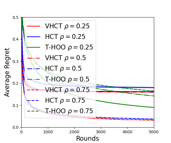
Synthetic Experiments. In Figure 4, we provide the performances of the different algorithms (VHCT, HCT, T-HOO) that need the smoothness parameters under different parameter settings ρ{0.25,0.5,0.75}\rho\in\{0.25,0.5,0.75\}. Here, we choose to plot an equivalent notion, the average regret Rt/tR_{t}/t instead of the cumulative regret RtR_{t} because some curves have very large cumulative regrets, so it would be hard to compare them with the other curves. In general, ρ=0.75\rho=0.75 or ρ=0.5\rho=0.5 are good choices for VHCT and HCT, and ρ=0.25\rho=0.25 is a good choice for T-HOO. Therefore, we use these parameter settings in the real-life experiments and the additional experiments in the next subsection. For POO and PCT, we follow Grill et al. [2015] and use ρmax=0.9\rho_{\max}=0.9. The unknown bound bb is set to be b=1b=1 for all the algorithms used in the experiments.

Refer to caption
(a) Garland
Refer to caption
(b) DoubleSine
Refer to caption
(c) 2D-Rastrigin
Figure 4: Best parameters on the Garland, DoubleSine and Rastrigin function

Landmine Dataset. The landmine dataset contains 29 landmine fields, with each field consisting of different number of positions. Each position has some features extracted from radar images, and machine learning models (like SVM) are used to learn the features and detect whether a certain position has landmine or not. The dataset is available at http://www.ee.duke.edu/~lcarin/LandmineData.zip. We have followed the open-source implementation at https://github.com/daizhongxiang/Federated_Bayesian_Optimization to process the data and train the SVM model. We tune two hyper-parameters when training SVM, the RBF kernel parameter from [0.01, 10], and the L2L_{2} regularization from [1e-4, 10]. The model is trained on the training set with the selected hyper-parameter and then evaluated on the testing set. The testing AUC-ROC score is the blackbox objective to be optimized.

MNIST Dataset and Neural Network. The MNIST dataset can be downloaded from http://yann.lecun.com/exdb/mnist/ and is one of the most famous image classification datasets. We have used stochastic gradient descent (SGD) to train a two-layer feed-forward neural network on the training images, and the objective is the validation accuracy on the testing images. We have used ReLU activation and the hidden layer has 64 units. We tune three different hyper-parameters of SGD to find the best hyper-parameter, specifically, the mini batch-size from [1, 100], the learning rate from [1e-6, 1], and the weight decay from [1e-6, 5e-1].

E.2 Additional Experiments

In this subsection, we provide additional experiments on some other nonconvex optimization evaluation benchmarks. They are used in many optimization researches to evaluate the performance of different optimization algorithms, including the convergence rate, the precision and the robustness such as Azar et al. [2014], Shang et al. [2019], Bartlett et al. [2019]. Detailed discussions of these functions can be found at https://en.wikipedia.org/wiki/Test_functions_for_optimization Although some of these function values (e.g., the Himmelblau function) are not bounded in [0,1][0,1] on the domain we select, the convergence rate of different algorithms will not change as long as the function is uniformly bounded over its domain. To commit a fair comparison (i.e., sharing similar signal/noise ratio), we have re-scaled all the objectives listed below to be bounded by [1,1][-1,1].

We list the functions used and their mathematical expressions as follows.

  • DoubleSine (Figure 5(a)) is (originally) a one dimensional function proposed by Grill et al. [2015] with multiple sharp local minimums and one global minimum. The results are shown in Figure 1(a).

    f(x,y)=20exp[0.20.5(x2+y2)]+exp[0.5(cos2πx+cos2πy)]e20.f(x,y)=20\exp\left[-0.2\sqrt{0.5\left(x^{2}+y^{2}\right)}\right]+\exp[0.5(\cos 2\pi x+\cos 2\pi y)]-e-20.
  • The counter example f(x)=1+1/lnxf(x)=1+1/\ln x in 4 decreases too fast around zero and thus its smoothness cannot be measured by ν1ρh\nu_{1}\rho^{h} for any constants ν1,ρ>0\nu_{1},\rho>0. However, because it is continuously differentiable and even monotone, the function is very easy to optimize. The results are shown in Figure 6(b).

  • Himmelbalu (Figure 5(c)) is (originally) a two dimensional function with four flat global minimums. We use the negative of the original function for maximization, and we restrain xx to be in [5,5]2[-5,5]^{2} to include all four global maximums. The results are shown in Figure 6(c).

    f(x,y)=(x2+y11)2(x+y27)2.f(x,y)=-\left(x^{2}+y-11\right)^{2}-\left(x+y^{2}-7\right)^{2}.
  • Rastrigin (Figure 5(d)) is a multi-dimensional function with a vast number of sharp local minimums and one global minimum. We use the negative of the original function for maximization. We run all the algorithms on the 10-dimensional space [1,1]10[-1,1]^{10}. The results are shown in Figure 6(d).

    f(𝐱)=An+i=1n[Acos(2πxi)xi2] with A=10.f(\mathbf{x})=-An+\sum_{i=1}^{n}\left[A\cos\left(2\pi x_{i}\right)-x_{i}^{2}\right]\text{ with }A=10.
Refer to caption
(a) DoubleSine
Refer to caption
(b) Counter Example
Refer to caption
(c) Himmelblau
Refer to caption
(d) 10D-Rastrigin
Figure 5: Plots of all the synthetic objectives used in the experiments. We have used a 10-dimensional Rastrigin function and the figure in (d) is a two-dimensional one.
Refer to caption
(a) DoubleSine
Refer to caption
(b) Counter Example
Refer to caption
(c) Himmelblau
Refer to caption
(d) 10D-Rastrigin
Figure 6: Cumulative regret of different algorithms on the synthetic functions.

As can be observed in all the figures, VHCT is one of the fastest algorithms, which validates our claims in the theoretical analysis. We remark that Himmelblau is very smooth after the normalization by its maximum absolute value on [5,5]2[-5,5]^{2} (890) and thus a relatively easier task compared with functions such as Rastrigin. DoubleSine contain many local optimums that are very close to the global optimum. Therefore, the regret differences between VHCT and HCT are expected to be small in these two cases.

E.3 Performance of VHCT in the High-noise Setting

Apart from the low-noise setting, we have also examined the performance of 𝚅𝙷𝙲𝚃\mathtt{VHCT} in the high-noise setting. In the following experiments, we have set the noise to be ϵtUniform(0.5,0.5)\epsilon_{t}\sim\text{Uniform}(-0.5,0.5). Note that the function values are in [1,1][-1,1], therefore such a noise is very high. As discussed in Section 4.4, it should be expected that the performance of 𝚅𝙷𝙲𝚃\mathtt{VHCT} is similar to or only marginally better than 𝙷𝙲𝚃\mathtt{HCT} in this case. As shown in Figure 7, the performance of 𝚅𝙷𝙲𝚃\mathtt{VHCT} and 𝙷𝙲𝚃\mathtt{HCT} are similar, which matches our expectation.

Refer to caption
(a) Garland
Refer to caption
(b) DoubleSine
Refer to caption
(c) Himmelblau
Refer to caption
(d) 1D-Rastrigin
Figure 7: Performance of different algorithms on the synthetic functions with high noise