Optimizing dividends and capital injections limited by bankruptcy, and practical approximations for the Cramér-Lundberg process
Abstract
The recent papers Gajek-Kucinsky(2017) and Avram-Goreac-Li-Wu(2020) investigated the control problem of optimizing dividends when limiting capital injections stopped upon bankruptcy. The first paper works under the spectrally negative Lévy model; the second works under the Cramér-Lundberg model with exponential jumps, where the results are considerably more explicit. The current paper has three purposes. First, it illustrates the fact that quite reasonable approximations of the general problem may be obtained using the particular exponential case studied in Avram-Goreac-Li-Wu(2020). Secondly, it extends the results to the case when a final penalty is taken into consideration as well besides a proportional cost for capital injections. This requires amending the “scale and Gerber-Shiu functions" already introduced in Gajek-Kucinsky(2017). Thirdly, in the exponential case, the results will be made even more explicit by employing the Lambert-W function. This tool has particular importance in computational aspects and can be employed in theoretical aspects such as asymptotics.
Keywords: dividend problem, capital injections, penalty at default, scale functions, Lambert-W function, De Vylder-type approximations, rational Laplace transform
1 Introduction
This paper concerns the approximate optimization of a new type of boundary mechanism, which emerged recently in the actuarial literature [APY18, GK17, AGLW20], in the context of the optimal control of dividends and capital injections.
The model. Consider the spectrally negative Lévy risk model:
where is a spectrally positive Lévy process, with Lévy measure . The classic example is that of the perturbed Cramèr-Lundberg risk model with
where is a Brownian motion, where is an independent Poisson process of intensity , and is a family of i.i.d.r.v. whose distribution, density and moments are denoted respectively by . Furthermore,
-
•
the process is modified by dividends and capital injection:
where are adapted, non-decreasing and càdlàg processes, with ;
-
•
the first time when we do not bail-out to positive reserves is called bankruptcy/absolute ruin;
-
•
prior to bankruptcy, dividends are limited by the available reserves: . The set of “admissible" policies satisfying this constraint will be denoted by .
The objective is to maximize the profit:
The value function is
Motivation. The recent papers [GK17, AGLW20] investigated the above control problem of optimizing dividends and capital injections for processes with jumps, when bankruptcy is allowed as well. The second paper works under the Cramér-Lundberg model with exponential jumps, while the first works under the spectrally negative Lévy model, allowing also for the presence of Brownian motion and infinite activity jumps. It turns out that the optimal policy belongs to the class of “bounded buffer policies", which consist in allowing only capital injections smaller than a given and declaring bankruptcy at the first time when the size of the overshoot below 0 exceeds and in paying dividends when the reserve reaches an upper barrier . These will briefly be described as policies from now on. Furthermore, the optimal are the roots of one variable equations with explicit solutions related to the Lambert-W(right) function (ProductLog in Mathematica).
Below, our goal is to show numerically that exponential approximations provide quite reasonable results (as the de Vylder approximation provides for the ruin problem). We will focus in our examples on the case of matrix exponential jumps(which are known to be dense in the class of general nonnegative jumps, with even error bounds for completely monotone jumps being available [VAVZ14]), for two reasons. One is in order to highlight certain exact equations which are similar to their exponential versions, and which may at their turn be used to produce even more accurate approximations in the future, and, secondly, since numerical Laplace inversion for this class may easily tuned to have arbitrarily small errors.
History of the problem: The case of no capital injections (also characterized by or absorption below 0) is the dividend problem posed by De Finetti [DF57, Ger69] where dividends are paid above barrier and is imposed. “The challenge is to find the right compromise between paying early in view of the discounting or paying late in order not to reach ruin too early and thus profit from the positive safety loading for a longer time" [AAM20].
Forced injections and no bankruptcy at (also characterized by a reflection at ) is studied in Shreve [SLG84] where dividends are paid above barrier and is imposed.
From Lokka, Zervos, [LZ08] we know that in the Brownian motion case, it is optimal to either always inject, if , for some critical cost (i.e. use Shreve), or, stop at (use De Finetti). We propose to call this the Lokka, Zervos alternative. The “proof" of this alternative starts by largely assuming it via a heuristically justified border Ansatz [LZ08, (5.2)]:
Extensive literature on SLG forced bailouts (no bankruptcy) can be found at Avram et al., (2007) [APP07], Kulenko and Schmidli, (2008) [KS08], Eisenberg and Schmidli, (2011) [ES11], Pérez et al., (2018) [PYB18], Lindensjo, Lindskog (2019) [LL19], Noba et al., 2020 [NPY20].
Articles [GK17, AGLW20] are the only papers which relate declaring bankruptcy to the size of jumps, with general and exponential jumps, respectively. [GK17] deals also with the presence of Brownian motion and infinite activity jumps, by conditioning at the first draw-down time; the optimality proof is quite involved.
In [AGLW20], it is also shown that neither nor are possible: the Lokka-Zervos alternative disappears, but another interesting alternative holds. Above a certain critical the optimal dividends barrier switches from strictly positive to , and is related in (26) to the Lambert-W function .
The results of [GK17, AGLW20] may be divided in three parts:
-
1.
Compute the value of bounded buffer policies. The key result is (5) below, an explicit determination of the objective , which allows optimizing it numerically.
REMARK 1.
Computing the value function is considerably simplified by the use of first passage recipes available for spectrally negative Lévy processes [AKP04, Kyp14, KKR13, AGVA19], which are built around two ingredients: the and -scale functions, defined respectively for as:
-
(a)
the inverse Laplace transform of , where is the Laplace exponent (which characterizes a Lévy process) and
-
(b)
– see the papers [Sup76, Ber98, AKP04] for the first appearance of these functions. The name -scale/harmonic functions is justified by the fact that these functions are harmonic for the process killed upon entering , in the sense that
are martingales, as shown in [Pis04, Prop. 3] (in the case of , there is also a penalty of at ruin, generalizing to other penalties produces the so-called Gerber-Shiu function).
-
(a)
-
2.
Equations determining candidates for the optimal are obtained by differentiating the objective (which is expressed in terms of the scale functions ), and the optimal pair is identified. As a result, the critical is related in (26) to the Lambert-W function.
-
3.
The optimality of the policy is established.
Note that the last step is quite non-trivial and is achieved by different methods in [GK17] and [AGLW20]. The latter paper starts by formulating a (new) HJB equation associated to this stochastic control problem – see (8).
REMARK 2.
The objective may be optimized numerically using the first step only (the equation (10) for ).
Exponential approximations may also be used, which are similar in spirit with the de Vylder-type approximations. Recall that the philosophy of the de Vylder approximation is to approximate a Cramèr-Lundberg process by a simpler process with exponential jumps, with cleverly chosen exponential rate , and the parameters may also be modified, if one desires to make the approximations exact at –see for example [AHPS19] for more details)
The efficiency of the de Vylder approximation for approximating ruin probabilities is well documented [DV78]. The natural question of whether this type of techniques may work for other objectives, like for example for optimizing dividends and/or reinsurance was already discussed in [Høj02, DD05, BDW07, GSS08, AHPS19]. In this paper, following on previous works [ACFH11, AP14, ABH18], we draw first the attention to the fact that we have not one, but three de Vylder-type approximations for (as for the ruin probability). The best approximation in our experiments when the loading coefficient is large turn out to be the classic de Vylder approximation. However, for approximating near the origin, the two point Padé approximation which fixes both the values works better. The end result here is simply replacing the inverse rate by in the formula for the scale function of the Cramèr-Lundberg process with exponential jumps. In between and , the winner is sometimes the “Renyi approximation" which replaces the inverse rate by , and modifies as well (for the de Vylder approximation, is replaced by , and both are modified).
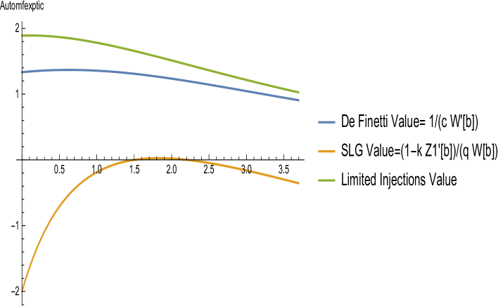
We end this introduction by highlighting in figure 1 the fact that for exponential jumps, the limited capital injections objective function given by (14) for arbitrary but optimal (via a complicated formula) improves the value function with respect to de Finetti and Shreve, Lehoczky and Gaver, for any .
Contents and contributions. Section 2 offers a conjectured profit formula for policies, where we include also a final penalty . The theoretical result of the section 1 revisits [GK17, AGLW20] by linking the two formulations together and emphasizing the impact of the bankruptcy penalty (via the scale function ). Its proof is beyond the scope of the present (already lengthy enough) paper and it can be inferred from either one of [GK17] and [AGLW20] through a three step argument:
-
1.
express the cost by conditioning on the reserve () starting from hitting either 0 or b;
-
2.
get a further relationship on costs and by conditioning on the first claim;
-
3.
finally, mix these conditions together in order to obtain the explicit formula for .
We also wish to point out (in section 2.1) the link to an appropriate HJB variational inequality equation8 and the definition 1 specifying the action regions and their computation starting from the regimes in the HJB system. To the best of our knowledge, this is new and the preliminary studies conducted on more complicated problems (involving reinsurance and reserve-dependent premium) seem to reinforce the relevance of this tool.
In section 7 we provide an alternative matrix exponential form of the exact cost, in the case of matrix exponential jumps.
An explicit determination of and an equity cost dichotomy when dealing with exponential jumps are given in section 3, taking also advantage of properties of the Lambert-W function, which were not exploited before. The two main novelties of the section are:
- •
- •
Again, a further novelty is the presence of the bankruptcy cost .
Section 4 reviews, for completeness, the de Vylder approximation-type approximations. Section 4.1 recalls, for warm-up, some of the oldest exponential approximations for ruin probabilities. Section 4.2 recalls in Proposition 5, following [AP14, AHPS19] three approximations of the scale function 444essentially, this is the “dividend function with fixed barrier”, which had been also extensively studied in previous literature before the introduction of , obtained by approximating its Laplace transform. These amount finally to replacing our process by one with exponential jumps and cleverly crafted parameters based on the first three moments of the claims.
In section 5, we consider particular examples and obtain very good approximations for two fundamental objects of interest: the growth exponent of the scale function , and the (last) global minimum of , which is fundamental in the de Finetti barrier problem. Proceeding afterwards to the problem of dividends and limited capital injections, concepts in section 3 are used to compute a straightforward exponential approximation based on an exponential approximation of the claim density, and a new “correct ingredients approximation" which consists of plugging into the objective function (10) for exponential claims the exact "non-exponential ingredients" (scale functions and, survival and mean functions) of the non-exponential densities. Both methods are observed to yield reasonable values in approximating the objective.
This leads us to our conclusion that from a practical point of view, exponential approximations are typically sufficient in the problems discussed in this paper.
2 The cost function of policies, for the spectrally negative Lévy case
In this section, we allow to be a spectrally positive Lévy process, with a Lévy measure admitting a density . The simplest example is that of the perturbed Cramèr-Lundberg risk model with
where is a Poisson process of intensity , is an independent family of i.i.d.r.v. with density , and is an independent Brownian motion.
We revisit here the problem of optimizing the value of "bounded buffer policies", following [GK17, AGLW20] (in order to relate the results, one needs to replace in the objective of [GK17] by ), while taking into account also the bankruptcy penalty .
An important role in the results will be played by the expected scale after a jump
| (1) |
where is the tail of the Lévy measure and is the Brownian volatility (the identity above follows easily from the -harmonicity of , after an integration by parts of the convolution term and a division by ).
The problem of limited reflection requires introducing a new "scale function and Gerber-Shiu function "– see Remark 4 for further comments on this terminology:
| (2) |
where
EXAMPLE 1.
With exponential jumps and possibly , using the identities
we find that the functions (2) are expressible as products of and the survival or mean function of the jumps:
| (3) |
([GK17] use , instead of , respectively). When , these reduce to quantities in [AGLW20].
The formulas above will be used below as a heuristic approximation in non-exponential cases.
REMARK 3.
Note that
| (4) |
and that are increasing functions in .
We state now a generalization of [GK17, Thm. 4] for the value function of policies, in terms of . In the Cramèr-Lundberg case illustrated below, the proof is straightforward, following [AGLW20]. In the other case, one needs to adapt the proof of [GK17].
THEOREM 1.
Cost function for policies For a spectrally negative Lévy processes, let
denote the expected discounted dividends minus capital injections associated to policies consisting in paying capital injections with proportional cost , provided that the severity of ruin is smaller than , and paying dividends as soon as the process reaches some upper level . Put
Then, it holds that
| (5) |
REMARK 4.
The first equality in (5) will be easily obtained by applying the strong Markov property at the stopping time , but it still contains the unknown .
This relation suggests a definition of the scale and the Gerber-Shiu function , as the coefficient of and the part independent of , respectively.
This equality is also equivalent to
| (6) |
which suggests another analytic definition of the scale and Gerber-Shiu function corresponding to an objective which involves reflection at .
The functions may be shown to stay the same for problems which require only modifying the boundary condition at , like the problem of capital injections for the process reflected at , or the problem of dividends for the process reflected at , with proportional retention (this is in coherence with previously studied problems).
COROLLARY 2.
Let us consider the Cramèr-Lundberg setting without diffusion (i.e. ), For fixed , the optimality equation may be written as
| (7) |
REMARK 5.
The first equality in (7) provides a relation between the objective and the variable ; the second recognizes this as the smooth fit equation .
Proof: Recalling the expressions of , , in (6), in (2), and from [GK17, Lem. A.4]
where denote derivatives with respect to the subscript , Whenever , if achieves the maximum in , it is straightforward (think of the economic interpretation) that achieves the maximum of for every . Therefore, we find
∎
2.1 The HJB System
The optimality proof in [AGLW20] is based on showing that the function (5) with defined in (18), (19) is the minimal AC-supersolution of the HJB system
| (8) |
where the Hamiltonian is given by
| (9) |
To discuss (8), it is useful to introduce the concept of dividend-limited injections strategies and barrier strategies. The following are also valid for its generalizations to mixed singular/continuous controls taking into account reinsurance:
DEFINITION 1.
Dividend-limited injections strategies are stationary strategies where the dividends are paid according to a partition of the state space in five sets as follows:
-
1.
If the surplus is in (absolute ruin), bankruptcy is declared and a penalty is paid;
-
2.
If the surplus is in bailouts/capital injections are used for bringing the surplus to the closest point of .
-
3.
If the surplus is in the open set (continuation/no action set), no controls are used.
-
4.
If the current surplus is in (these are upper-accumulation points of ), dividends are paid at a positive rate, in order to keep the surplus process from moving.
-
5.
If the current surplus is in , a positive amount of money is paid as dividends in order to bring the surplus process to .
Barrier strategies are stationary strategies for which are four consecutive intervals.
REMARK 6.
REMARK 7.
One may conjecture that dividend-limited injections strategies are of a (recursive) multi-band nature. In the case of exponential jumps, [AGLW20] show that the four sets in the optimal solution are intervals, denoted respectively by .
Cheap equity corresponds the case when , and the partition reduces to three sets.
3 Explicit determination of when
In this section we turn to the exponential case, where explicit formulas for the optimizers are available. In particular, we will take advantage of properties of the Lambert-W function, which were not exploited in [AGLW20]. Subsequently, in sections 5, 6 we will show that exponential approximations work typically excellently in the general case. Although these results have already been established in [AGLW20], the present formulations have two achievements:
- 1.
-
2.
make use of a numerical tool (Lambert-W function) to express the optimal quantities of interest .
3.1 The simplified cost function and optimality equations
PROPOSITION 3.
Cost function and optimality equations in the exponential case
-
1.
(10) where we put
-
2.
Put
(11) For fixed , the optimality equation may be written as
(12) -
3.
For fixed and , at critical points with satisfies we must have
Explicitly,
(13) -
4.
When and is fixed, the solution of (13) may be expressed in terms of the principal value of the “Lambert-W(right)" function (an inverse of )
[CGH+96, Boy98, BFS08, Pak15, VLSHGG+19] (this observation is missing in [AGLW20]).
(14) It follows that
(15) - 5.
-
6.
At a critical point , we must have both
(18) and
(19) -
7.
The equation may be solved explicitly for , yielding
(20)
Proof: 1. follows from Theorem 1.1.
2. Let denote the numerator an denominator of in (10). The optimality equation simplifies to
3. (13) is a consequence of 1 and of the smooth fit result Corollary 2.
4. See the proof of the particular case 5; holds since
6. follows from 2. and .3.
7. is straightforward.
∎
REMARK 8.
Note that the de Finetti and Shreve, Lehoczky and Gaver solutions are always non-optimal, when (see (14)).
However, as , and, . This suffices to infer that you get de Finetti case.
On the other hand,
| (21) |
Thus, these regimes can be recovered asymptotically. Let now denote the unique roots of in the two asymptotic cases, which coincide with the classic Shreve, Lehoczky and Gaver and de Finetti barriers.
Then, it may be checked that .
3.2 Existence of the roots of the equations
The following (new) result discusses the existence of the roots of the equations introduced in proposition (3) and relates them to the Lambert-W function.
PROPOSITION 4.
-
1.
increases from to , as we see it in the figure below.

Figure 2: Plot of with and , for , and . is increasing-decreasing (from to ), with a maximum at the unique root of given by
(22) where denote the positive and negative roots of the Cramèr-Lundberg equation .
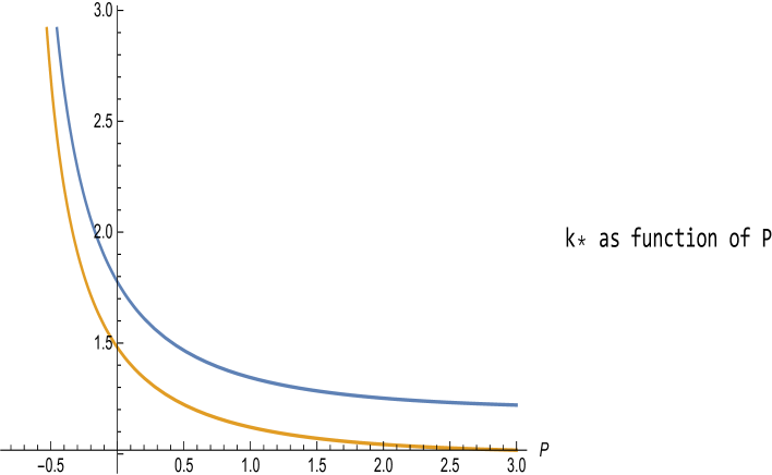
The figure below illustrates the plot of the function and in which the is represented by the black point.

Figure 3: Plots of and with and , for , and . 
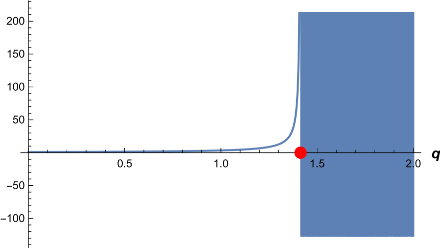
Figure 4: For , and , the root of is at -
2.
Put
(24) and assume
(25) Then, , the function is decreasing in with , and has a unique root
(26) where
(27) (note that the denominator does not equal since and takes always values bigger than ; or, note that , where is the other real branch of the Lambert function).
Furthermore,
(28) -
3.
It follows that has at least one solution of in iff
(29) The first such solution will be denoted by .
Proof: For 1. see [AGLW20, Proof of Theorem 11, A2].
2. By using the assumption we get , and is decreasing.
Put . The inequality (see (29)) may be reduced to
Rewriting the latter as we recognize, by putting , an inequality reducible to The solution is
where is the principal branch of the Lambert-W function.
The final solution is (28), where we may note that the variables have been separated.
3. is straightforward.
∎
REMARK 9.
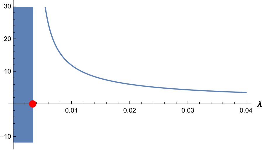
The function blows up at , and converges to when (or when either or are large enough) as may be noticed in the figure below, which blows up at the value Note also that when (or one of are large enough), given by (26) stabilizes to the equilibrium ; this is related to [APP07, Lemma 2], [KS08, Lemma 7], who obtain the same condition for (without buffering capital injections). Intuitively, under these conditions, buffering is not crucial.
At the other end, as tends to its lower limit and to the regime B, the notion of equity expensiveness vanishes, and .
The next two figures illustrate how blows up at the critical values and (represented by red points in the figures below). The dark (blue) parts correspond to the regime .
4 Which exponential approximation?
4.1 Three de Vylder-type exponential approximations for the ruin probability
In the simplest case of exponential jumps of rate and , the formula for the ruin probability is
| (30) |
where is the loading coefficient. By plugging the correct mean of the claims in the second formula yields the simplest approximation for processes with finite mean claims.
More sophisticated is the Renyi exponential approximation
| (31) |
This formula can be obtained as a two point Padé approximation of the Laplace transform, which conserves also the value [AP14]. It may be also derived heuristically from the first formula in (30), via replacing by the correct “excess mean" of the excess/severity density
which is known to be . Heuristically, it makes more sense to approximate instead of the original density , since is a monotone function, and also an important component of the Pollaczek-Khinchine formula for the Laplace transform – see [Ram92, AP14].
More moments are put to work in the de Vylder approximation
| (32) |
Interestingly, the result may be expressed in terms of the so-called "normalized moments"
| (33) |
introduced in [BHT05].
The de Vylder approximation parameters above may be obtained either from
The second derivation via Padé shows that higher order approximations may be easily obtained as well. They might not be admissible, due to negative values, but packages for “repairing" the non-admissibility are available – see for example [DcSA16].
The first derivation of the de Vylder approximation is a process approximation (i.e., independent of the problem considered); as such, it may be applied to other functionals of interest besides ruin probabilities(, dividend barriers, etc), simply by plugging the modified parameters in the exact formula for the ruin probability of the simpler process.
4.2 Three two point Padé approximations of the Laplace transform of scale function
The simplest approximations for the scale function will now be derived heuristically from the following example.
EXAMPLE 2.
The Cramér-Lundberg model with exponential jumps Consider the Cramér-Lundberg model with exponential jump sizes with mean , jump rate , premium rate , and Laplace exponent . Solving for yields two distinct solutions given by
The scale function is:
| (34) |
where .
Plugging now the respective parameters of the de Vylder type approximations in the exact formula (34) for the Cramèr-Lundberg process with exponential claims, we obtain three approximations for :
- 1.
-
2.
Renyi 444This is called DeVylder B) method in [GSS08, (5.6-5.7)], since it is the result of fitting the first two cumulants of the risk process. , obtained by plugging (since is unchanged, the latter equation is equivalent to the conservation of and to the conservation of , so this coincides with the Renyi ruin approximation used in (31).)
-
3.
De Vylder, obtained by plugging .
REMARK 10.
In the case of exponential claims, these three approximations are exact, by definition (or check that for exponential claims all the normalized moments are equal to ).
REMARK 11.
The conditions for the non-negativity of the barrier is . Here, this condition is satisfied for the exact when .
It is shown in [AHPS19, Prop. 1] that the three de Vylder type approximations are two-point Padé approximations of the Laplace transform (hence higher order generalizations are immediately available).
We recall that two-point Padé approximations incorporate into the Padé approximation two initial values of the function (which can be derived easily via the initial value theorem, from the Pollaczek-Khinchine Laplace transform):
| (36) | |||
| (37) |
In our case, incorporating both leads to the natural exponential approximation which is therefore the best near . Incorporating none of them yields the de Vylder approximation, which is the best asymptotically. Incorporating only leads to Renyi, which is expected to be the best in an intermediate regime.
Note that when the jump distribution has a density , it holds that : 666This equation is important in establishing the nonnegativity of the optimal dividends barrier.
| (38) |
Thus, already requires knowing (which is a rather delicate task starting from real data); therefore we will not incorporate into the Padé approximation more than two initial values of the function.
We recall below in Proposition 5 three types of two-point Padé approximations [AHPS19, Prop. 1], and particularize them to the case when the denominator degree is (which are further illustrated below).
PROPOSITION 5.
Three matrix exponential approximations for the scale function.
- 1.
-
2.
To ensure only , we must use the Padé approximation
For , we find
(40) where is the first moment of the excess density . Note that it equals the scale function of a process with exponential claims of rate and with modified to . Since is unchanged, the latter equation is equivalent to the conservation of and to the conservation of , so this coincides with the Renyi approximation 444This is called DeVylder B) method in [GSS08, (5.6-5.7)], since it is the result of fitting the first two cumulants of the risk process. used in (31).
-
3.
The pure Padé approximation yields for
Note that both the coefficient of in the denominator coincides with the coefficient in the classic de Vylder approximation, since , and so does the coefficient of , since
5 Examples of computations involving scale function and dividend value approximations
Our goal in this section is to investigate whether exponential approximations are precise enough to yield reasonable estimates for quantities important in control like
-
1.
the dominant exponent of
-
2.
the last local minimum of , , which yields, when being the global minimum, the optimal De Finetti barrier
-
3.
, which determines if
-
4.
the functional yielding the maximum dividends with capital injections.
All the examples considered involve a Cramèr-Lundberg model with rational Laplace transform (since in this case, the computation of is fast and in principle arbitrarily large precision may be achieved with symbolic algebra systems).
-
1.
For the first three problems, we will use de Vylder type approximations. Graphs of , and some tables summarizing the simulation results will be presented. We note that in most of the cases that we observed, the de Vylder approximation of deviates from the exact value the least – see for example Table 2. For the De Finetti barrier, the "winner" depends on the size of . Unsurprisingly, when near , the natural exponential approximation wins, and as increases, Renyi and subsequently the de Vylder approximation take the upper hand – see for example Table 3.
-
2.
For the computation of , we provide, besides the exact value, also two approximations:
-
(a)
For a given density of claims one computes an exponential density approximation where is the first moment of . Subsequently, , , and are obtained using the exponential approximation . Quantities obtained by this method would be referred to with an affix ‘expo pure’.
-
(b)
For a given density of claims , the value function is computed via the formula which assumes exponential claims in equation 3, but the "ingredients" , and the mean function are the correct ingredients corresponding to our original density . Quantities obtained by this method would be referred to with an affix ‘expo CI’.
It turns out that the pure expo approximation works better for large , and the correct ingredients approximation works better for small .
Note that we only included tables illustrating approximating for the first two examples, to keep the length of the paper under control, but similar results were obtained for the other examples.
-
(a)
5.1 A Cramér-Lundberg process with hyperexponential claims of order 2
We take a look at a Cramér-Lundberg process with density function with , and .
|
|
|
|
|||||||||
|---|---|---|---|---|---|---|---|---|---|---|---|---|
| Exact | 0.110113 | 0 | 3.45398 | 0 | ||||||||
| Expo | 0.110657 | 0.494313 | 3.51173 | 1.67191 | ||||||||
| Dev | 0.110115 | 0.00195933 | 3.48756 | 0.972251 | ||||||||
| Renyi | 0.110078 | 0.0321413 | 3.5323 | 2.26744 |
| Closest approximation | exact | approximation | % error | |
|---|---|---|---|---|
| 1 | Dev | 0.110113 | 0.110115 | 0.00195933 |
| 0.9 | Dev | 0.120328 | 0.120331 | 0.00269878 |
| 0.8 | Dev | 0.132452 | 0.132457 | 0.00380056 |
| 0.7 | Dev | 0.147017 | 0.147025 | 0.00548411 |
| 0.6 | Dev | 0.16475 | 0.164763 | 0.00812643 |
| 0.5 | Dev | 0.186652 | 0.186675 | 0.0123901 |
| 0.4 | Dev | 0.214122 | 0.214163 | 0.0194631 |
| 0.3 | Dev | 0.249118 | 0.249196 | 0.0315039 |
| 0.2 | Dev | 0.294396 | 0.294551 | 0.0524528 |
| 0.1 | Dev | 0.353829 | 0.354145 | 0.0894466 |
| Closest approximation | Barrier exact | Barrier approx | % error Barrier | |
| 1 | Dev | 3.45398 | 3.48756 | 0.972251 |
| 0.9 | Dev | 3.20191 | 3.23103 | 0.909487 |
| 0.8 | Dev | 2.90951 | 2.93074 | 0.729628 |
| 0.7 | Dev | 2.57043 | 2.57742 | 0.272088 |
| 0.6 | Dev | 2.1804 | 2.16054 | 0.910666 |
| 0.5 | Ren | 1.74216 | 1.75266 | 0.60278 |
| 0.4 | Expo | 1.2735 | 1.29456 | 1.65378 |
| 0.3 | Expo | 0.81068 | 0.652264 | 19.5412 |
| J0 | |||||
|---|---|---|---|---|---|
| J0 exact | J0 expo pure | J0 expo pure error | J0 expo CI | J0 expo CI error | |
| 1 | 5.95034 | 5.99151 | 0.691856 | 6.26009 | 5.20551 |
| 0.9 | 5.15579 | 5.17573 | 0.386663 | 5.45269 | 5.7584 |
| 0.8 | 4.39383 | 4.38494 | 0.202205 | 4.67042 | 6.29489 |
| 0.7 | 3.68299 | 3.63933 | 1.18555 | 3.92937 | 6.68958 |
| 0.6 | 3.04577 | 2.96728 | 2.57704 | 3.25112 | 6.7423 |
| 0.5 | 2.50331 | 2.39942 | 4.15022 | 2.65901 | 6.21974 |
| 0.4 | 2.06833 | 1.9585 | 5.31006 | 2.17044 | 4.93725 |
| 0.3 | 1.74095 | 1.65616 | 4.86984 | 1.78984 | 2.80878 |
| 0.2 | 1.50439 | 1.44242 | 4.11969 | 1.50871 | 0.286672 |
| 0.1 | 1.30271 | 1.25324 | 3.79748 | 1.30271 | 0 |
| a | |||||
|---|---|---|---|---|---|
| a exact | a expo pure | a expo pure error | a expo CI | a expo CI error | |
| 1 | 3.9669 | 3.99434 | 0.691861 | 4.17339 | 5.20551 |
| 0.9 | 3.4372 | 3.45049 | 0.386665 | 3.63512 | 5.7584 |
| 0.8 | 2.92922 | 2.9233 | 0.202204 | 3.11361 | 6.29489 |
| 0.7 | 2.45533 | 2.42622 | 1.18555 | 2.61958 | 6.68958 |
| 0.6 | 2.03051 | 1.97818 | 2.57704 | 2.16741 | 6.7423 |
| 0.5 | 1.66888 | 1.59961 | 4.15022 | 1.77268 | 6.21974 |
| 0.4 | 1.37888 | 1.30566 | 5.31006 | 1.44696 | 4.93725 |
| 0.3 | 1.16063 | 1.10411 | 4.86983 | 1.19323 | 2.80878 |
| 0.2 | 1.00293 | 0.961612 | 4.11969 | 1.0058 | 0.286672 |
| 0.1 | 0.868476 | 0.835496 | 3.79748 | 0.868476 | 0 |
| b | |||||
| b exact | b expo pure | b expo pure error | b expo CI | b expo CI error | |
| 1 | 1.41036 | 1.46188 | 3.65293 | 1.25374 | 11.1045 |
| 0.9 | 1.37645 | 1.44439 | 4.93621 | 1.23362 | 10.3761 |
| 0.8 | 1.31492 | 1.40417 | 6.78809 | 1.19529 | 9.09781 |
| 0.7 | 1.21057 | 1.32258 | 9.25207 | 1.12775 | 6.84178 |
| 0.6 | 1.04634 | 1.17215 | 12.0245 | 1.01753 | 2.7529 |
| 0.5 | 0.810767 | 0.920406 | 13.5229 | 0.853397 | 5.25805 |
| 0.4 | 0.510085 | 0.538725 | 5.61475 | 0.634716 | 24.4335 |
| 0.3 | 0.17425 | 0.0105496 | 93.9457 | 0.376872 | 116.282 |
| 0.2 | 0 | 0 | 0 | 0.105322 | 100 |
| 0.1 | 0 | 0 | 0 | 0 | 0 |
5.2 A Cramér-Lundberg process with hyperexponential claims of order 3
Consider a Cramér-Lundberg process with density function , and , , , , .
The Laplace exponent of this process is and from this one can invert to obtain the scale function 222Laplace inversion done via Mathematica; coefficients and exponents are decimal approximations of the real values.
From this, we see that the dominant exponent is .
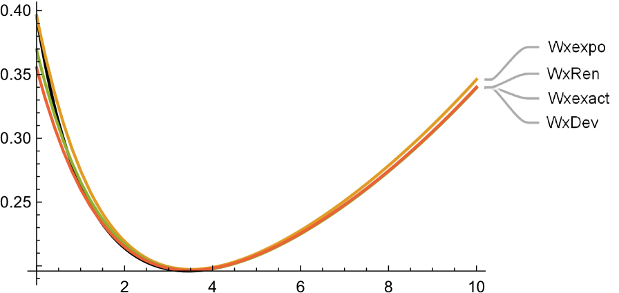
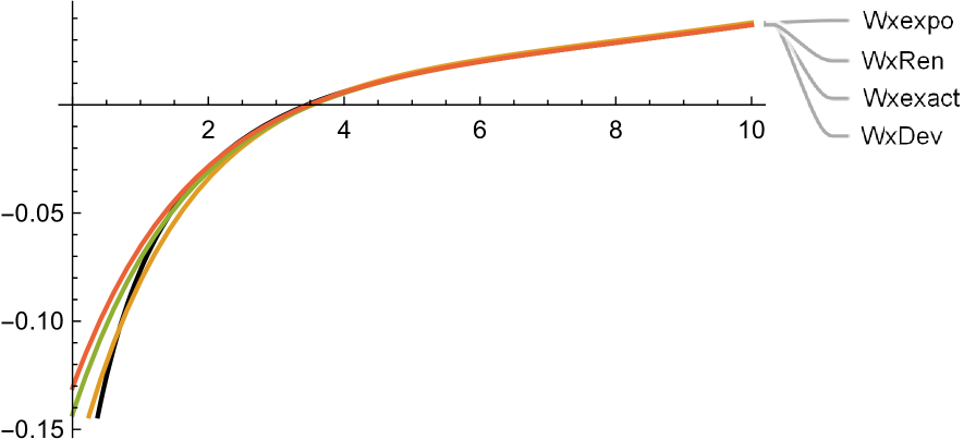
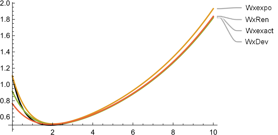
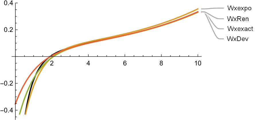
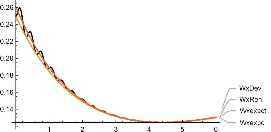
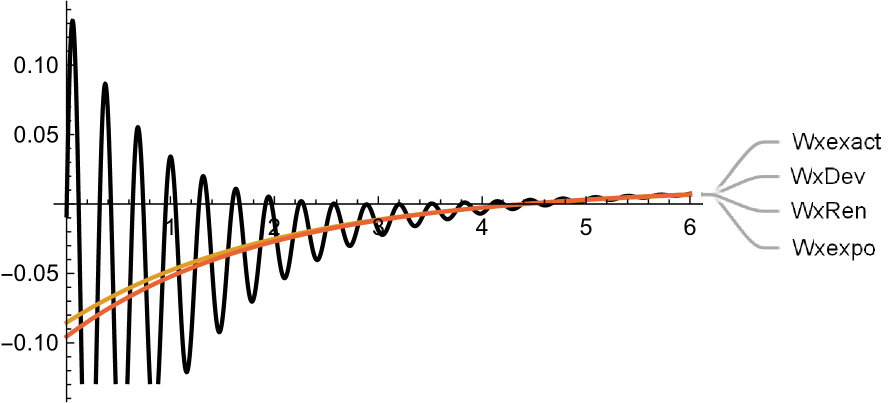
Figure 8 shows the exact and approximate plots of the first two derivatives of . The exact plots are labelled Wxexact, and coloured as the darkest. The plots of exhibit noticeable unique minima around , with the exact one being at , which is the optimal barrier that maximizes dividends here. Note that the approximations are practically indistinguishable from the exact around this point (which is our main object of interest here).
|
|
|
|
|||||||||
|---|---|---|---|---|---|---|---|---|---|---|---|---|
| Exact | 0.18198 | 0 | 1.89732 | 0 | ||||||||
| Expo | 0.184095 | 1.162215628 | 2.04608 | 7.840532962 | ||||||||
| Renyi | 0.181708 | 0.149466974 | 2.08136 | 9.699997892 | ||||||||
| Dev | 0.182011 | 0.017034839 | 1.91233 | 0.79111589 |
| Closest approximation | exact | approximation | % error | |
|---|---|---|---|---|
| 263/235 | Dev | 0.18198 | 0.182011 | 0.0168217 |
| 243/235 | Dev | 0.194712 | 0.194754 | 0.0213671 |
| 223/235 | Dev | 0.209221 | 0.209279 | 0.0274827 |
| 203/235 | Dev | 0.225876 | 0.225957 | 0.0358309 |
| 183/235 | Dev | 0.245146 | 0.245262 | 0.0474032 |
| 163/235 | Dev | 0.267635 | 0.267806 | 0.0637063 |
| 143/235 | Dev | 0.294126 | 0.294382 | 0.0870647 |
| 123/235 | Dev | 0.325643 | 0.326038 | 0.121115 |
| 103/235 | Dev | 0.363539 | 0.364163 | 0.171618 |
| 83/235 | Dev | 0.40961 | 0.410625 | 0.247788 |
| 63/235 | Dev | 0.466261 | 0.46796 | 0.364457 |
| 43/235 | Dev | 0.536719 | 0.539647 | 0.545532 |
| 23/235 | Dev | 0.62533 | 0.630516 | 0.829419 |
| 3/235 | Dev | 0.737962 | 0.747389 | 1.27736 |
| Closest approximation | Barrier exact | Barrier approx | % error Barrier | |
| 263/235 | Dev | 1.89732 | 1.91233 | 0.791183 |
| 243/235 | Dev | 1.79954 | 1.78002 | 1.08482 |
| 183/235 | Ren | 1.45224 | 1.52484 | 4.9989 |
| 163/235 | Ren | 1.31579 | 1.33691 | 1.60463 |
| 143/235 | Ren | 1.16804 | 1.12368 | 3.79796 |
| 123/235 | Expo | 1.00898 | 1.04123 | 3.19653 |
| 103/235 | Expo | 0.839228 | 0.794964 | 5.27444 |
| 83/235 | Expo | 0.660338 | 0.513179 | 22.2854 |
| 63/235 | Expo | 0.474896 | 0.196234 | 58.6785 |
| 43/235 | Expo | 0.286563 | 0 | 100 |
| 23/235 | Expo | 0.0998863 | 0 | 100 |
| 3/235 | All | 0 | 0 | 0 |
We move now to the dividend problem with capital injections with cost as in Theorem 1. One can compute the value function at in terms of , ,, , and – see equation 5.
To provide a more concrete example, fixing ,, as input parameters we compute for values of as a function of , with results summarized in the tables below. The tables provide comparisons of the computed optimal quantities , , and to an approximation using all exponential inputs (referred to as , , and expo pure) and to an approximation which uses actual inputs but computed using the exponential formula as described in equation 3 (referred to as , , and expo CI).
| J0 | |||||
|---|---|---|---|---|---|
| expo pure | expo pure error | expo CI | expo CI error | ||
| 263/235 | 3.7747 | 3.76883 | 0.155556 | 4.11784 | 9.09041 |
| 243/235 | 3.41491 | 3.38603 | 0.845606 | 3.74156 | 9.5654 |
| 223/235 | 3.0636 | 3.00802 | 1.81444 | 3.36985 | 9.99637 |
| 203/235 | 2.72335 | 2.63828 | 3.1238 | 3.00466 | 10.3296 |
| 183/235 | 2.39737 | 2.28225 | 4.80185 | 2.64879 | 10.4871 |
| 163/235 | 2.08958 | 1.94765 | 6.79226 | 2.3062 | 10.3665 |
| 143/235 | 1.80446 | 1.64396 | 8.8946 | 1.9823 | 9.85516 |
| 123/235 | 1.54668 | 1.38072 | 10.73 | 1.68379 | 8.86472 |
| 103/235 | 1.32041 | 1.16526 | 11.7499 | 1.4178 | 7.37587 |
| 83/235 | 1.12864 | 1.00194 | 11.2258 | 1.19022 | 5.45555 |
| 63/235 | 0.972835 | 0.88785 | 8.73585 | 1.00404 | 3.20798 |
| 43/235 | 0.852739 | 0.789923 | 7.36635 | 0.859039 | 0.738837 |
| 23/235 | 0.751597 | 0.701299 | 6.69218 | 0.751597 | 0 |
| 3/235 | 0.660372 | 0.620567 | 6.02761 | 0.660372 | 0 |
| a | |||||
|---|---|---|---|---|---|
| expo pure | expo pure error | expo CI | expo CI error | ||
| 263/235 | 2.51647 | 2.74523 | 0.155536 | 2.51255 | 9.09042 |
| 243/235 | 2.27661 | 2.49437 | 0.845596 | 2.25735 | 9.56541 |
| 223/235 | 2.0424 | 2.24657 | 1.81443 | 2.00535 | 9.99638 |
| 203/235 | 1.81557 | 2.00311 | 3.1238 | 1.75885 | 10.3296 |
| 183/235 | 1.59825 | 1.76586 | 4.80185 | 1.5215 | 10.4871 |
| 163/235 | 1.39306 | 1.53747 | 6.79226 | 1.29844 | 10.3665 |
| 143/235 | 1.20298 | 1.32153 | 8.8946 | 1.09598 | 9.85516 |
| 123/235 | 1.03112 | 1.12252 | 10.73 | 0.920479 | 8.86472 |
| 103/235 | 0.880271 | 0.945198 | 11.7499 | 0.77684 | 7.37587 |
| 83/235 | 0.752428 | 0.793477 | 11.2258 | 0.667962 | 5.45555 |
| 63/235 | 0.648557 | 0.669362 | 8.73585 | 0.5919 | 3.20798 |
| 43/235 | 0.568493 | 0.572693 | 7.36635 | 0.526616 | 0.738838 |
| 23/235 | 0.501065 | 0.501065 | 6.69218 | 0.467532 | 0 |
| 3/235 | 0.440248 | 0.440248 | 6.02761 | 0.413711 | 0 |
| b | |||||
|---|---|---|---|---|---|
| expo pure | expo pure error | expo CI | expo CI error | ||
| 263/235 | 0.709355 | 0.805116 | 13.4997 | 0.677918 | 4.43179 |
| 243/235 | 0.695874 | 0.801936 | 15.2416 | 0.671779 | 3.46259 |
| 223/235 | 0.677601 | 0.794377 | 17.2337 | 0.662801 | 2.18425 |
| 203/235 | 0.653005 | 0.779265 | 19.3352 | 0.649805 | 0.490147 |
| 183/235 | 0.620126 | 0.751601 | 21.2012 | 0.631097 | 1.76912 |
| 163/235 | 0.576553 | 0.704104 | 22.123 | 0.604293 | 4.81128 |
| 143/235 | 0.519526 | 0.627369 | 20.7579 | 0.566198 | 8.98366 |
| 123/235 | 0.446259 | 0.511076 | 14.5246 | 0.512961 | 14.947 |
| 103/235 | 0.354524 | 0.346046 | 2.39143 | 0.440755 | 24.3231 |
| 83/235 | 0.243362 | 0.126054 | 48.2032 | 0.347059 | 42.6099 |
| 63/235 | 0.113593 | 0 | 100 | 0.231975 | 104.216 |
| 43/235 | 0 | 0 | 0 | 0.0987484 | 0 |
| 23/235 | 0 | 0 | 0 | 0 | 0 |
| 3/235 | 0 | 0 | 0 | 0 | 0 |
To provide a point of comparison, we fix , and compute the de Finetti barrier to be and the corresponding dividend value function when starting at to be .
| % deviation | % deviation | ||||
|---|---|---|---|---|---|
| 1 | 154.123 | 3.0801 | 5.07857 | 100 | 0 |
| 2 | 65.714 | 1.31327 | 3.31174 | 43.0208 | 1.08108 |
| 3 | 42.863 | 0.856604 | 2.85507 | 25.4792 | 1.4139 |
| 4 | 31.4465 | 0.628448 | 2.62692 | 17.6853 | 1.56178 |
| 5 | 24.6995 | 0.493611 | 2.49208 | 13.4234 | 1.64264 |
| 6 | 20.2855 | 0.4054 | 2.40387 | 10.7759 | 1.69287 |
| 7 | 17.1884 | 0.343504 | 2.34197 | 8.98441 | 1.72686 |
| 8 | 14.9014 | 0.2978 | 2.29627 | 7.69619 | 1.7513 |
| 9 | 13.1463 | 0.262724 | 2.26119 | 6.72732 | 1.76968 |
| 10 | 11.758 | 0.23498 | 2.23345 | 5.97306 | 1.78399 |
| 100 | 1.11095 | 0.0222019 | 2.02067 | 0.533448 | 1.8872 |
| 1000 | 0.110409 | 0.00220648 | 2.00067 | 0.0527257 | 1.89632 |
| 10000 | 0.0109536 | 0.000218903 | 1.99869 | 0.00533526 | 1.89722 |
5.3 A Cramér-Lundberg process with oscillating density and scale function
In the following example, we study a Cramèr-Lundberg model with density of claims given by
where
Assuming further that , , , and that , , the Laplace exponent for this process is and the scale function is
|
|
|
|
|||||||||
|---|---|---|---|---|---|---|---|---|---|---|---|---|
| Exact | 0.0881484 | 0 | 4.38201 | 0 | ||||||||
| Expo | 0.0878658 | 0.32053 | 4.42263 | 0.927122 | ||||||||
| Renyi | 0.0881481 | 0.000314617 | 4.39788 | 0.362284 | ||||||||
| Dev | 0.0881484 | 6.11743*10^-6 | 4.39745 | 0.352331 |
Clearly, our completely monotone approximation cannot fully reproduce functions like in examples like this where oscillations occur (note however that the de Finetti optimal barrier is well approximated here). If a more exact reproduction is necessary, higher order approximations should be used.
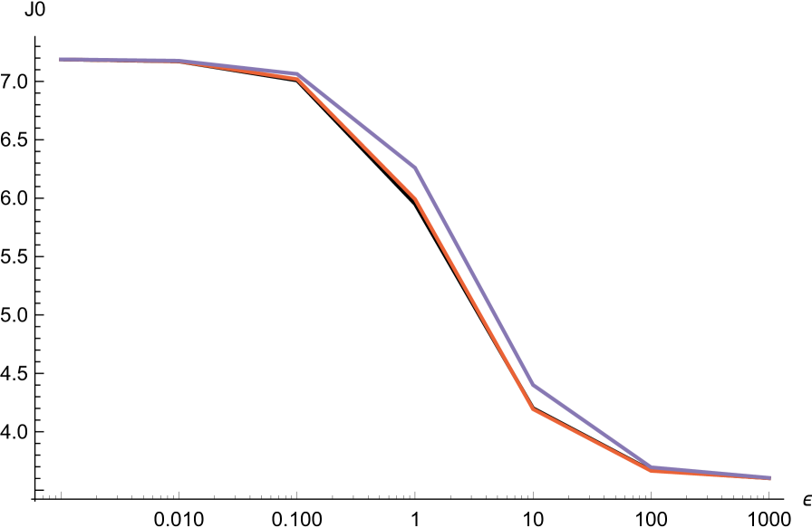
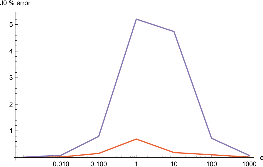
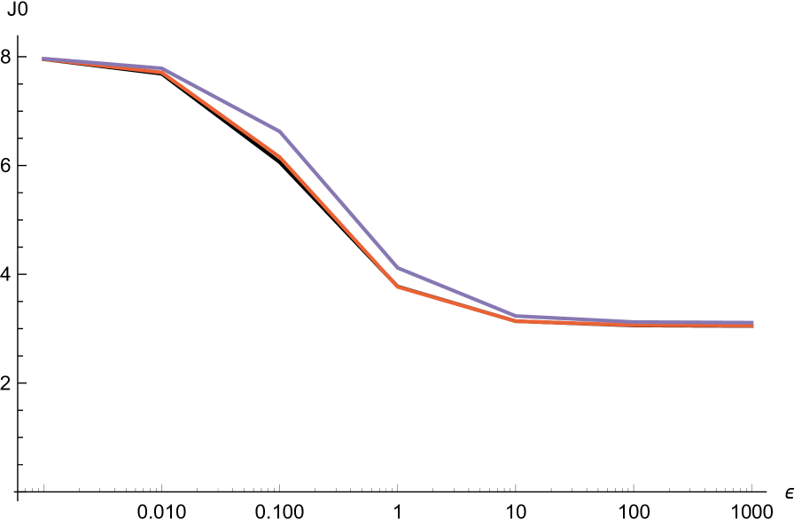
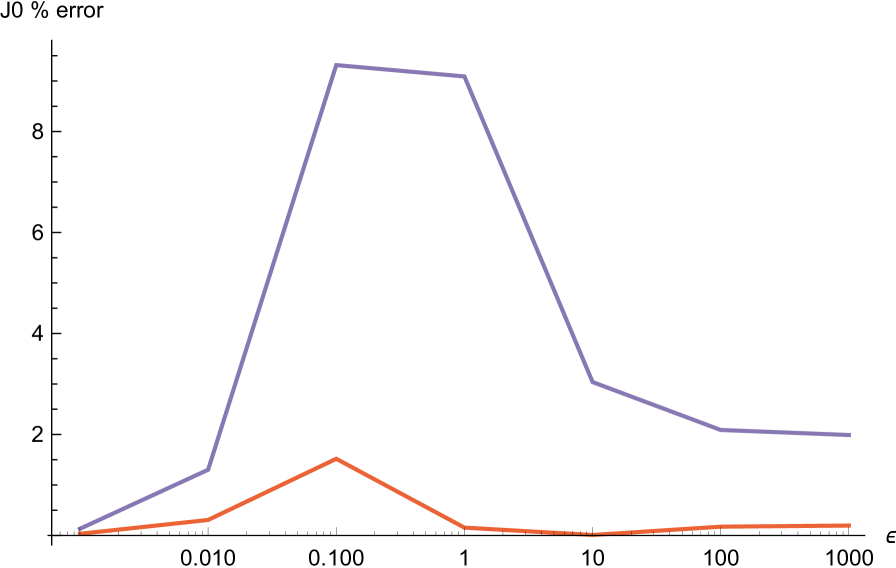
6 The maximal error of exponential approximations along one parameter families of Cramér-Lundberg processes
In this section, we provide the two approximations for the dividend value with capital injections , and the dividend barrier , for two one parameter families of Cramér-Lundberg processes, with densities given respectively by:
| (41) | |||
| (42) |
where is the normalization constant, and compute the maximal error of approximation when and . For this choice, the pure exponential approximation works considerably better, .
| J0 | |||||
|---|---|---|---|---|---|
| J0 exact | J0 expo pure | J0 expo pure error | J0 expo CI | J0 expo CI error | |
| 0.001 | 7.1879 | 7.18802 | 0.0016603 | 7.18849 | 0.00827967 |
| 0.01 | 7.17075 | 7.17193 | 0.0164663 | 7.17666 | 0.0824782 |
| 0.1 | 7.008 | 7.01863 | 0.151653 | 7.06358 | 0.793041 |
| 1 | 5.95034 | 5.99151 | 0.691856 | 6.26009 | 5.20551 |
| 10 | 4.20175 | 4.19406 | 0.183122 | 4.40089 | 4.73941 |
| 100 | 3.66909 | 3.6654 | 0.100631 | 3.69555 | 0.721228 |
| 1000 | 3.6025 | 3.60208 | 0.0117065 | 3.60523 | 0.075585 |
We do the same thing for the family of densities given by .
| J0 | |||||
|---|---|---|---|---|---|
| J0 exact | J0 expo pure | J0 expo pure error | J0 expo CI | J0 expo CI error | |
| 0.001 | 7.95508 | 7.95771 | 0.0330111 | 7.96565 | 0.132796 |
| 0.01 | 7.68765 | 7.71127 | 0.307292 | 7.78772 | 1.30166 |
| 0.1 | 6.06176 | 6.15381 | 1.5186 | 6.62641 | 9.31507 |
| 1 | 3.7747 | 3.76883 | 0.155556 | 4.11784 | 9.09041 |
| 10 | 3.1382 | 3.1379 | 0.00959692 | 3.23354 | 3.03813 |
| 100 | 3.05894 | 3.06427 | 0.174306 | 3.12284 | 2.08921 |
| 1000 | 3.0508 | 3.05678 | 0.196219 | 3.11149 | 1.98956 |
7 The profit function when the claims are distributed according to a matrix exponential jumps density
Consider now the more general case when the claims are distributed according to a matrix exponential density generated by a row vector and by an invertible matrix of order , which are such that the vector is decreasing componentwise to , and , with a column vector. As customary, we restrict w.l.o.g. to the case when is a probability vector, and , so that
is a valid survival function.
The matrix versions of our functions are:
| (43) |
where
| (44) |
The product formulas (43) may also be established directly in the phase-type case, using the conditional independence of the ruin probability of the overshoot size.
We derive first these extensions from scratch for phase-type densities, in order to highlight their probabilistic interpretation. Later, we will show that the matrix exponential jumps case follows as a particular case of [GK17].
Recall first [AA10] that where is a vector whose components represent the probability that ruin occurs during a certain phase, and that the conditional independence of ruin and overshoots translates into the product formula
| (45) |
To take advantage of this, it is convenient to replace from the beginning by , taking advantage of the formula [AKP04, Kyp14]
| (46) |
Alternatively, one may introduce a vector function
| (47) |
On the other hand, the mean function may be written as
The following result follows in the phase-type case just as in the exponential case [AGLW20]; in the matrix exponential jumps case, it may be obtained from [GK17]:
PROPOSITION 6.
For a Cramèr-Lundberg process (compound Poisson ) with matrix exponential jumps of type , it holds that
-
1.
(48) where
(49) and
(50) -
2.
For fixed , the optimality equation simplifies to
(51)
REMARK 12.
The additive separation of which was the basis of proving optimality in the exponential case does not seem possible anymore, but (50) allows the numeric computation of the optimum.
References
- [AA10] Hansjörg Albrecher and Sören Asmussen, Ruin probabilities, vol. 14, World Scientific, 2010.
- [AAM20] Hansjoerg Albrecher, Pablo Azcue, and Nora Muler, Optimal ratcheting of dividends in insurance, SIAM Journal on Control and Optimization 58 (2020), no. 4, 1822–1845.
- [ABH18] Florin Avram, Abhijit Datta Banik, and András Horváth, Ruin probabilities by Padé’s method: simple moments based mixed exponential approximations (Renyi, De Vylder, Cramér–Lundberg), and high precision approximations with both light and heavy tails, European Actuarial Journal (2018), 1–27.
- [ACFH11] Florin Avram, Donatien Chedom-Fotso, and András Horváth, On moments based Padé approximations of ruin probabilities, Journal of Computational and Applied mathematics 235 (2011), no. 10, 3215–3228.
- [AGLW20] Florin Avram, D. Goreac, J Li, and X Wu, Equity cost induced dichotomy for optimal dividends in the cramér-lundberg model, IME (2020).
- [AGVA19] Florin Avram, D. Grahovac, and C. Vardar-Acar, The scale functions kit for first passage problems of spectrally negative Lévy processes, and applications to the optimization of dividends, arXiv preprint (2019).
- [AHPS19] Florin Avram, Andras Horváth, Serge Provost, and Ulyses Solon, On the padé and laguerre–tricomi–weeks moments based approximations of the scale function w and of the optimal dividends barrier for spectrally negative lévy risk processes, Risks 7 (2019), no. 4, 121.
- [AKP04] Florin Avram, Andreas Kyprianou, and Martijn Pistorius, Exit problems for spectrally negative Lévy processes and applications to (Canadized) Russian options, The Annals of Applied Probability 14 (2004), no. 1, 215–238.
- [AM14] Pablo Azcue and Nora Muler, Stochastic optimization in insurance: A dynamic programming approach, Springer, 2014.
- [AP14] Florin Avram and Martijn Pistorius, On matrix exponential approximations of ruin probabilities for the classic and brownian perturbed cramér-lundberg processes, Insurance: Mathematics and Economics 59 (2014), 57–64.
- [APP07] Florin Avram, Zbigniew Palmowski, and Martijn R Pistorius, On the optimal dividend problem for a spectrally negative Lévy process, The Annals of Applied Probability (2007), 156–180.
- [APY18] Florin Avram, José Luis Pérez, and Kazutoshi Yamazaki, Spectrally negative Lévy processes with Parisian reflection below and classical reflection above, Stochastic processes and Applications 128 (2018), 255–290.
- [BDW07] Christopher J Beveridge, David CM Dickson, and Xueyuan Wu, Optimal dividends under reinsurance, Centre for Actuarial Studies, Department of Economics, University of …, 2007.
- [Ber98] Jean Bertoin, Lévy processes, vol. 121, Cambridge university press, 1998.
- [BFS08] PB Brito, F Fabiao, and A Staubyn, Euler, lambert, and the lambert w-function today., Mathematical Scientist 33 (2008), no. 2.
- [BHT05] Andrea Bobbio, András Horváth, and Miklós Telek, Matching three moments with minimal acyclic phase type distributions, Stochastic models 21 (2005), no. 2-3, 303–326.
- [Boy98] JP Boyd, Global approximations to the principal real-valued branch of the lambert w-function, Applied mathematics letters 11 (1998), no. 6, 27–31.
- [CGH+96] Robert M Corless, Gaston H Gonnet, David EG Hare, David J Jeffrey, and Donald E Knuth, On the lambertw function, Advances in Computational mathematics 5 (1996), no. 1, 329–359.
- [DD05] David Dickson and Steve Drekic, Optimal dividends under a ruin probabilityconstraint, 2005.
- [DF57] Bruno De Finetti, Su un’impostazione alternativa della teoria collettiva del rischio, Transactions of the XVth international congress of Actuaries, vol. 2, 1957, pp. 433–443.
- [DcSA16] Bogdan Dumitrescu, Bogdan C cSicleru, and Florin Avram, Modeling probability densities with sums of exponentials via polynomial approximation, Journal of Computational and Applied Mathematics 292 (2016), 513–525.
- [DV78] Fl De Vylder, A practical solution to the problem of ultimate ruin probability, Scandinavian Actuarial Journal 1978 (1978), no. 2, 114–119.
- [ES11] Julia Eisenberg and Hanspeter Schmidli, Minimising expected discounted capital injections by reinsurance in a classical risk model, Scandinavian Actuarial Journal 2011 (2011), no. 3, 155–176.
- [Ger69] Hans U Gerber, Entscheidungskriterien für den zusammengesetzten poisson-prozess, Ph.D. thesis, ETH Zurich, 1969.
- [GK17] Leslaw Gajek and Lukasz Kuciński, Complete discounted cash flow valuation, Insurance: Mathematics and Economics 73 (2017), 1–19.
- [GSS08] Hans U Gerber, Elias SW Shiu, and Nathaniel Smith, Methods for estimating the optimal dividend barrier and the probability of ruin, Insurance: Mathematics and Economics 42 (2008), no. 1, 243–254.
- [Høj02] Bjarne Højgaard, Optimal dynamic premium control in non-life insurance. maximizing dividend pay-outs, Scandinavian Actuarial Journal 2002 (2002), no. 4, 225–245.
- [KKR13] Alexey Kuznetsov, Andreas E Kyprianou, and Victor Rivero, The theory of scale functions for spectrally negative Lévy processes, Lévy Matters II, Springer, 2013, pp. 97–186.
- [KS08] Natalie Kulenko and Hanspeter Schmidli, Optimal dividend strategies in a cramér–lundberg model with capital injections, Insurance: Mathematics and Economics 43 (2008), no. 2, 270–278.
- [Kyp14] Andreas Kyprianou, Fluctuations of Lévy processes with applications: Introductory lectures, Springer Science & Business Media, 2014.
- [LL19] Kristoffer Lindensjö and Filip Lindskog, Optimal dividends and capital injection under dividend restrictions, arXiv preprint arXiv:1902.06294 (2019).
- [LZ08] Arne Løkka and Mihail Zervos, Optimal dividend and issuance of equity policies in the presence of proportional costs, Insurance: Mathematics and Economics 42 (2008), no. 3, 954–961.
- [NPY20] Kei Noba, José-Luis Pérez, and Xiang Yu, On the bailout dividend problem for spectrally negative markov additive models, SIAM Journal on Control and Optimization 58 (2020), no. 2, 1049–1076.
- [Pak15] Anthony G Pakes, Lambert’s w meets kermack–mckendrick epidemics, IMA Journal of Applied Mathematics 80 (2015), no. 5, 1368–1386.
- [Pis04] Martijn R Pistorius, On exit and ergodicity of the spectrally one-sided Lévy process reflected at its infimum, Journal of Theoretical Probability 17 (2004), no. 1, 183–220.
- [PYB18] José-Luis Pérez, Kazutoshi Yamazaki, and Alain Bensoussan, Optimal periodic replenishment policies for spectrally positive Lévy demand processes, arXiv preprint arXiv:1806.09216 (2018).
- [Ram92] Colin M Ramsay, A practical algorithm for approximating the probability of ruin, Transactions of the Society of Actuaries 44 (1992), 443–461.
- [SLG84] Steven E Shreve, John P Lehoczky, and Donald P Gaver, Optimal consumption for general diffusions with absorbing and reflecting barriers, SIAM Journal on Control and Optimization 22 (1984), no. 1, 55–75.
- [Sup76] VN Suprun, Problem of destruction and resolvent of a terminating process with independent increments, Ukrainian Mathematical Journal 28 (1976), no. 1, 39–51.
- [VAVZ14] Eleni Vatamidou, Ivo Jean Baptiste Franccois Adan, Maria Vlasiou, and Bert Zwart, On the accuracy of phase-type approximations of heavy-tailed risk models, Scandinavian Actuarial Journal 2014 (2014), no. 6, 510–534.
- [VLSHGG+19] H Vazquez-Leal, MA Sandoval-Hernandez, JL Garcia-Gervacio, AL Herrera-May, and UA Filobello-Nino, Psem approximations for both branches of lambert function with applications, Discrete Dynamics in Nature and Society 2019 (2019).