Optimized protocols for duplex quantum transduction
Abstract
Quantum transducers convert quantum signals through hybrid interfaces of physical platforms in quantum networks. Modeled as quantum communication channels, performance of unidirectional quantum transduction can be measured by the quantum channel capacity. However, characterizing performance of quantum transducers used for duplex quantum transduction where signals are converted bidirectionally remains an open question. Here, we propose rate regions to characterize the performance of duplex quantum transduction. Using this tool, we find that quantum transducers optimized for simultaneous duplex transduction can outperform strategies based on the standard protocol of time-shared unidirectional transduction. Integrated over the frequency domain, we demonstrate that rate region can also characterize quantum transducers with finite bandwidth.
Introduction.—Quantum transducers convert quantum signals between physically distinct carriers, enabling quantum information exchange across multiple platforms in quantum networks Kimble (2008). For example, a microwave-to-optical quantum transducer Lambert et al. (2020); Han et al. (2021); Andrews et al. (2014); Vainsencher et al. (2016); Fan et al. (2018); Rueda et al. (2019); Jiang et al. (2020); Mirhosseini et al. (2020); McKenna et al. (2020); Xu et al. (2021); Tu et al. (2022); Shen et al. (2022) can distribute processed quantum states stored in superconducting qubits over optical fibers. Various designs of quantum transducers have been developed, utilizing hybrid interfaces like electro-optics Tsang (2010); Fan et al. (2018); Rueda et al. (2019); McKenna et al. (2020); Xu et al. (2021), optomechanics Aspelmeyer et al. (2014); Stannigel et al. (2010); Safavi-Naeini and Painter (2011); Hill et al. (2012); Palomaki et al. (2013); Andrews et al. (2014); Lecocq et al. (2016); Vainsencher et al. (2016); Jiang et al. (2020); Mirhosseini et al. (2020); Shen et al. (2022), and electro-magnonics Zhang et al. (2014); Tabuchi et al. (2015); Shen et al. (2022).
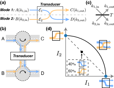
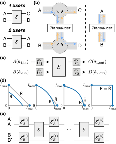
As devices for quantum state transfer, quantum transducers can be abstracted as quantum channels. Most bosonic quantum transducers use red-detuned pumps Han et al. (2021); Andrews et al. (2014); Fan et al. (2018); Rueda et al. (2019); Jiang et al. (2020); Mirhosseini et al. (2020); McKenna et al. (2020) to engineer a two-mode scattering process that is equivalent to a beam splitter. The input signal of one mode gets converted to the output signal of the other mode , yielding two unidirectional transduction channels and (Fig. 1(a)). Oftentimes, only a single channel is utilized to transduce quantum signal from one mode to the other, which we refer to as unidirectional quantum transduction. The performance of unidirectional quantum transduction is characterized by the quantum capacity of either or Zhang et al. (2018); Wang et al. (2022).
By leveraging both unidirectional transduction channels, quantum signals can be converted bidirectionally which we refer to as duplex quantum transduction 111Previous works on “bidirectional conversion” Andrews et al. (2014); Vainsencher et al. (2016); Jiang et al. (2020); Xu et al. (2021) measures the two unidirectional transduction channels separately on a single device, while the duplex quantum transduction we consider here is more general.. Duplex quantum transduction can be modeled as a quantum interference channel Fawzi et al. (2012); Sen (2012); Das et al. (2021), with senders and and receivers and . The senders and receivers can be distinct users by separating the input and output signals of each mode with circulators (Fig. 1(b)). For example, a lossless beam splitter with efficiency (Fig. 1(c)) implements a quantum interference channel:
| (1) |
One strategy for duplex quantum transduction is to alternate between using and , while simultaneous transduction of uncorrelated input signals and may be more efficient. However, and can interfere with each other when put in use simultaneously, e.g., the input signal for acts as added noise for in a beam splitter (Eq. (1)). As a result, characterizing the performance of duplex quantum transduction requires a new metric beyond the quantum capacities of the individual unidirectional transduction channels.
We propose to use achievable information rate region as the performance metric. The achievable rates of a quantum device depend on the quantum channels it implements as well as the input signal encodings, with channel parameters (such as in Eq. (1)) determined by the physical device parameters. In duplex quantum transduction, both transduction channels and transmit quantum information at rates and respectively. For simultaneous duplex transduction, the pair of achievable rates depends on how we encode quantum information into the quantum signals. By varying the encodings for and , we obtain a two-dimensional region of achievable information rates (Fig. 1(d)). The rate region characterizes the performance of simultaneous duplex transduction and its boundary indicates the optimized coding strategies. Past studies have also employed rate regions or capacity regions to study the trade-off among multiple quantum channels, albeit limited to sending classical information Bennett et al. (2003); Childs et al. (2006); Fawzi et al. (2012); Sen (2012); Shi et al. (2021) or distributing entanglement in qubit-based quantum networks Pant et al. (2019); Shi and Qian (2020); Vardoyan et al. (2021); Dai et al. (2022). So far, there is no analysis investigating the achievable quantum information rate region at the hardware level, such as quantum transducers.
Furthermore, we can combine simultaneous duplex transduction with the time-sharing strategy, where we alternate between different signal encodings and even device parameters. This leads to a new region of achievable rates that is the convex hull of the original region, and we refer to the new region as the time-sharing achievable rate region. For example, we can perform transduction in one direction with for 40% of the time and in the opposite direction with for the rest 60% of the time (black dot Fig. 1(d)). Notably, when the original region is not convex, time-sharing can offer additional performance boost for duplex quantum transduction.
In this work, we define the (time-sharing) achievable rate region and apply the tool to characterize the performance of two-mode quantum transducers. We demonstrate that a sizable portion of quantum transducers can benefit from simultaneously transducing quantum signals in both directions. We also discuss how reflectionless scattering leads to the optimal duplex quantum transduction, as well as the effect of finite bandwidth.
Rate regions of duplex quantum transduction.—We consider quantum transducers with a linear input-output relation
| (2) |
where the scattering matrix is unitary and depends on the device parameters of the transducer Han et al. (2021). We choose ports 1 and 2 as the signal ports, and are the injected vacuum noise from the internal loss channels. The two transduction channels are
| (3) |
Intuitively, the transmission coefficients and determine the transduction efficiency, while the reflection coefficients and lead to the interference between and .
Here we define the achievable information rates for simultaneous duplex transduction. For a quantum channel , the achievable rate of quantum information with an input state is measured by the coherent information Wilde (2013). Let be a purification of , we have
| (4) |
where is the von Neumann entropy of and is the identity map on . For , the achievable rate is 0. Generalizing to a quantum interference channel , the simultaneously achievable information rates with uncorrelated input state are
| (5) |
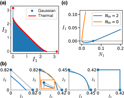
Given the challenges in determining the quantum capacity for lossy channels with added noise Schumacher and Nielsen (1996); Lloyd (1997); Devetak (2005); Weedbrook et al. (2012), we focus on the rate region achievable with thermal input states as a lower bound. When the input signals of and are thermal states with average photon number and , the outputs are also thermal states with photon number and (Fig. 2(a)). Here is the power reflection coefficient from port , is the power transmission coefficient from port to port , and we assume . For finite and , the reflected signal from one channel adds thermal noise to the other channel, which leads to the trade-off between and for simultaneous duplex transduction.
The achievable rates for Eq. (3) with thermal input states are (see Appendix A)
| (6) |
where ,
| (7) |
and
| (8) |
The rate region only depends on channel parameters . We could combine simultaneous duplex transduction with the time-sharing protocol, and the resulting time-sharing rate region is the convex hull . Additionally, numerical evidences suggest that thermal encodings are likely optimal among general Gaussian encodings (see Appendix A.1). The rate regions can be calculated similarly when the environment injects thermal noise rather than vacuum noise via the internal loss channels (see Appendix A.2).
The rate region can be determined from its boundary . For the special cases of unidirectional quantum transduction with and , we achieve information rates and on (Fig. 2(b), blue dots). Here is the quantum capacity of the pure-loss channel Holevo and Werner (2001). For and , corresponds to a continuous mapping and can be solved numerically with the low-rank Jacobian condition , where is the Jacobian matrix. In Fig. 2(b), we plot the rate regions (blue lines and dots) and (grey lines) for different reflection coefficients . We choose with .
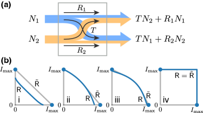
Finite reflection results in a noticeable discontinuity of the boundary at the axis (Fig. 2(b)i-iii). This can be explained from the upper bound on the thermal-loss capacity Rosati et al. (2018); Sharma et al. (2018); Noh et al. (2019). Assuming , the channel is a thermal loss channel with noise photon . From the upper bound Rosati et al. (2018); Sharma et al. (2018); Noh et al. (2019)
| (9) |
we must have to achieve a positive information rate . On the other hand, when the quantum capacity is achieved at , which leads to the discontinuity at .
If one side is reflectionless with , the discontinuity of vanishes at the axis (Fig. 2(b)ii axis). If both sides are reflectionless, there is no interference between the two transduction channels and the maximal square region can be achieved (Fig. 2(b)iv). Therefore it is possible to outperform the time-shared unidirectional transduction (Fig. 1(d) grey dashed line) with the simultaneous duplex transduction, as long as the reflection coefficients are small (Fig. 2(b)ii-iv).
So far we have only considered direct transduction without adaptive control Zhang et al. (2018) or shared entanglement Zhong et al. (2020a, b); Wu et al. (2021). In Appendix B, we briefly discuss duplex quantum transduction assisted with local operations and classical communication (LOCC), along with the scenario where the senders are the same as the receivers which allows the interference-based techniques Lau and Clerk (2019); Zhang et al. (2022).
Optimized transduction protocols.—Here we apply the tool of rate regions to analyze a physical transducer model. The channel parameters , and thus the achievable rates, depend on the device parameters of the transducer. We therefore generalize the achievable rate regions to include not only different signal encodings but also different device parameters. The boundary of the resulting rate region leads to optimized signal encodings and device parameters for the transducer.
We consider a transducer model for frequency conversion between two bosonic modes and (Fig. 3 (a)). The lab frame Hamiltonian is
| (10) |
where are the mode frequencies, is the pump frequency and is the interaction rate. An input signal at frequency in mode 1 gets converted to an output signal at frequency in mode 2, and vice versa. The Hamiltonian in the rotating frame of the signal is
| (11) |
where and .
Assuming mode has external (internal) loss rate , the scattering matrix only depends on the ratios (see Appendix D). In practice, the loss rates of two modes may differ by orders of magnitude, but the ratios and are often close Fan et al. (2018); McKenna et al. (2020); Xu et al. (2021). Therefore, we assume symmetric loss rates for simplicity and the more general case is discussed in Appendix D. The input-output relation is given by
| (12) |
where are the internal loss channels, and
| (13) |
Here is the identity matrix, and
| (14) |
We focus on optimizing the detunings of the transducer, while keeping other relevant parameters fixed. Besides the signal encodings , the achievable rates also depends on the device parameters . We therefore define the rate region as . The optimized signal encodings and detunings can be obtained from the boundary of the time-sharing rate region .
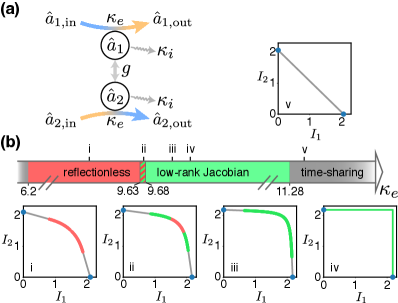
The boundary of the rate region can be determined by exploring several possible solutions. On the and axes, the quantum capacity of unidirectional quantum transduction increases with the transmission coefficient. Therefore we choose that leads to the highest transmission rate to achieve the information rates and on . For and , corresponds to a continuous mapping . The boundary as extreme values of the mapping can be obtained by comparing two possible solutions. One solution is from the low-rank Jacobian condition , where is the Jacobian matrix. The other solution is from the reflectionless condition with and where or . We consider this solution separately since the Jacobian matrix may be undefined under the limit of . The reflectionless solution can be calculated analytically. For example, requires
| (15) |
which leads to the achievable rates at
| (16) |
In practice, we expect an approximate reflectionless solution with and finite , due to input power constraints and uncertainties in controlling the reflection coefficients.
We calculate the time-sharing rate region for several choices of at and (Fig. 3(b)). The boundary may be composed of one or more types of the protocols: reflectionless (red), low-rank Jacobian (green) and time-sharing (grey). For example, for the boundary contains all three types of protocols (Fig. 3(b)ii) while for or the optimized protocols is time-shared unidirectional transduction. It is also worth mentioning that for the transducers benefit from the simultaneous duplex transduction.
If both and detunings are tunable, it can be proved that the highest transmission rate occurs when (see Appendix C). Therefore the optimal duplex quantum transduction is achieved with the two-side reflectionless condition at and (Fig. 3(b)iv). In other words, is the largest possible region in the sense that for any .
Frequency-integrated rate region.—Quantum transducer usually has a finite conversion bandwidth, which determines the range of signal frequencies that can be converted efficiently Zeuthen et al. (2020). Larger bandwidth enables higher operation speed of the transducer, and is preferable in presence of decoherence. Within the bandwidth, quantum signals at multiple frequencies can be transduced independently with frequency-dependent conversion efficiencies.
We can perform duplex quantum transduction in parallel for various signal frequencies, and the frequency-dependent scattering matrices result in distinct achievable rate regions that vary with frequency. Let for the transducer model Eq. (11), the signal detuning in the rotating frame becomes , and the frequency-dependent rate region is . We plot the time-sharing rate regions for multiple (Fig. 4(a)), and compare with the quantum capacity (Fig. 4(b)). For within the grey shaded region, simultaneous duplex transduction is advantageous, while outside this region time-shared unidirectional transduction is the optimal protocol.
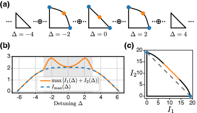
To obtain the total achievable rate region, we sum the contributions from the individual rate regions at each signal frequency (Fig. 4(a)). The frequency-integrated rate region for time-shared duplex transduction is defined as
| (17) |
where is a set of evenly spaced frequencies with a frequency spacing , and is the Minkowski sum De Berg et al. (2008) of two sets and . For general sets the complexity of Minkowski sum is , while for convex sets and in the complexity is De Berg et al. (2008). Therefore numerical evaluation of is efficient since is convex in .
We calculate the Minkowski sum of all rate regions in Fig. 4(a), and the resulting frequency-integrated rate region is shown in Fig. 4(c). The boundary can be achieved with frequency dependent protocols. For example, to realize the orange part of with a slope of -1, we choose the simultaneous duplex transduction protocol that maximizes (Fig. 4(a) orange dots) for signal detuning within the grey shaded region in Fig. 4(b). For other , we perform the time-shared unidirectional transduction. Benefiting from simultaneous duplex transduction, the frequency-integrated rate region outperforms the time-shared unidirectional transduction (Fig. 4(c) grey dashed line).
Discussion.—We proposed the (time-sharing) rate region to quantify the performance of duplex quantum transduction, and studied optimized protocols for a two-mode quantum transducer. Unlike unidirectional quantum transduction, duplex quantum transduction is influenced by the reflection coefficients, and we explored how the reflectionless condition can be related to the optimal duplex quantum transduction. Furthermore, we incorporated the finite bandwidth of the transducer and introduced the frequency-integrated rate region. In future works, it would be interesting to consider non-Gaussian encodings (see Appendix E), as well as other approaches to quantum transduction such as adaptive control Zhang et al. (2018), shared entanglement Zhong et al. (2020a, b); Wu et al. (2021) and interference-based methods Lau and Clerk (2019); Zhang et al. (2022). Our method can also be extended to analyze the performance of multiplex quantum hardware with more than two quantum channels, such as characterizing the performance of a 3-port quantum circulator with a 3-dimensional rate region. Exploring alternative performance metrics Siddiqui and Wilde (2022) for duplex quantum transduction may provide further insights.
Acknowledgements.
We thank Amir Safavi-Naeini, Cheng Guo, Chiao-Hsuan Wang, Mark M. Wilde and Siddhartha Das for helpful discussions. We acknowledge support from the ARO(W911NF-23-1-0077), ARO MURI (W911NF-21-1-0325), AFOSR MURI (FA9550-19-1-0399, FA9550-21-1-0209), AFRL (FA8649-21-P-0781), NSF (OMA-1936118, ERC-1941583, OMA-2137642), NTT Research, and the Packard Foundation (2020-71479). L.J. acknowledges the support from the Marshall and Arlene Bennett Family Research Program. This material is based upon work supported by the U.S. Department of Energy, Office of Science, National Quantum Information Science Research Centers.Appendix A Achievable rates of linear transducers
We provide details for the achievable rates Eq. (6) and discuss about the capacity region as well as rate region with general Gaussian states. The derivations are based on properties of Gaussian states and channels Weedbrook et al. (2012); Noh et al. (2019), and we follow the convention in Ref. Noh et al. (2019).
The transducer defined in Eq. (2) is a passive linear system, i.e., linear system without squeezing. Since is unitary, Eq. (2) is a Gaussian unitary transformation described by a symplectic matrix
| (18) |
with
| (19) |
where and we have defined the phase rotation matrix
| (20) |
The coherent information Eq. (4) can be calculated analytically for Gaussian input states. We choose a -mode Gaussian state with covariance matrix , where is the covariance matrix for mode . For quantum channel , we can purify the input state of mode 1 with a reference system. The joint covariance matrix of the reference system and mode 1 is
| (21) |
where
| (22) |
and the decomposition of general one-mode Gaussian states is
| (23) |
Here is the squeezing parameter and is the angle of the squeezing axis. We have defined and the single mode squeezing transformation .
The coherent information for channel is
| (24) |
where is the von Neumann entropy of a Gaussian state with covariance matrix , and
| (25) |
Here is the output state of mode 2 and is the joint output state of the reference system and mode 2.
We assume vacuum input states for modes with . In this case,
| (26) |
where we have used the fact that is unitary. Therefore only depends on and . Similarly, only depends on and . If the input states to mode 1 and 2 are thermal states instead of general Gaussian states, Eq. (24) reduces to Eq. (6) and the rate region only depends on .
A.1 Thermal states vs general Gaussian states
Let and be the rate regions achieved with thermal states and general Gaussian states respectively. Obviously . Below we prove that thermal states give rise to local optima of . Here we assume fixed channel parameters and the rate regions are obtained by varying the signal encodings.
Consider a mapping , where parametrizes the input states. A point is a local optimum if the two gradient vectors are in the opposite direction: with . For any small deviation around , the changes satisfy . Therefore if increases must decrease, and vice versa. Since and cannot be increased at the same time, is a local optimum. Notice that local optimum requires , which is stronger than the low-rank Jacobian condition since the low-rank Jacobian condition also includes .
For general Gaussian states , where are from the decomposition of (Eq. (23)). Notice that only depend on the relative angle between the two squeezing axes. This leads to the symmetry for , since and together is equivalent to rotating the squeezing axis by 90 degree which keeps unchanged. From this symmetry, we have
| (27) |
at for any .
For thermal states at the boundary , the gradient vectors must satisfy with . These thermal states correspond to general Gaussian states at , where the gradient vectors also satisfy with . This proves that thermal states are the local optima of .
We numerically calculate by sweeping (Fig. 5(a) blue region), and compare it with (Fig. 5(a) red line and red dots). The result gives , which indicates that thermal states are likely the global optima among general Gaussian states. The same conclusion also holds for other channel parameters that we tested.
A.2 Thermal noise from the internal loss channels
So far we have only considered vacuum noise injected from the internal loss channels, while thermal noises are common in practical devices, such as the pump-induced heating in microwave-optical quantum transducers Han et al. (2021). Here we take into account the effects of thermal noises by assuming all internal loss channels have average thermal occupation, i.e., . The more general situations where the internal loss channels have different thermal occupations can be studied similarly. The achievable rates under thermal noises are also given by Eq. (6), except now the output photon numbers are
| (28) |
We calculate the rate regions for in Fig. 6(b) at different transmission and reflection coefficients. The regions are much smaller than the ones with vacuum noise (main text Fig. 2(b)). The highest rates achievable with thermal states (Fig. 6(b) blue dots) are given by Holevo and Werner (2001)
| (29) |
where and .
With thermal noise, one-side reflectionless condition no longer leads to vanishing discontinuity of , which is different from the vacuum noise case. In the second subfigure of Fig. 6(b), we have while is still discontinuous at the axis (see inset). This is because to achieve the highest rate on the axis, we need to have minimal added thermal noise which requires . On the other hand, to achieve under thermal noise , must exceed some threshold that is larger than 0 (Fig. 6(c) blue dot).
Appendix B Different settings of duplex quantum transduction
In this section, we discuss a few different settings to operate a quantum transducer in the duplex scenario, based on the number of users involved and whether or not the transduction is assisted with LOCC.
4 users, no LOCC. In the main text, we focus on the 4-user setting, where the senders and are different from the receivers and (Fig. 6(a)). The 4-user setting can be realized by separating the input and output signal of each mode with a circulator (Fig. 6(b)). In this case, we could formally define the capacity region and study the symmetry of the capacity region.
The quantum capacity of a quantum channel is the maximal coherent information over all possible input states, including entangled states across multiple channel uses Schumacher and Nielsen (1996); Lloyd (1997); Devetak (2005). We can generalize quantum capacity to the capacity region for simultaneous duplex transduction. For a quantum interference channel , the capacity region is given by
| (30) |
for all with . Here is the space of density matrices on and are defined in Eq. (5).
Since the capacity region is invariant under arbitrary single-mode unitaries before and after the quantum channel (Fig. 6(c)), we can exploit this symmetry to obtain equivalent channels with the same capacity region. More specifically, we perform single-mode rotations which gives
| (31) |
where
| (32) |
We choose the rotation angles and the symplectic matrix becomes
| (33) |
where . Therefore, a scattering matrix has the same capacity region as a scattering matrix for the signal ports
| (34) |
4 users, with LOCC. We consider duplex quantum transduction in the 4-user setting where each transduction channel is assisted with LOCC. For a quantum channel , the LOCC-assisted capacity 222LOCC-assisted capacity is also known as “two-way capacity”, but we avoid the term “two-way” to prevent any confusion with “duplex” quantum transduction. is the maximal quantum information rate when the forward quantum channel is assisted with forward and backward classical communication Bennett et al. (1997). The LOCC-assisted capacity is lower bounded by the reverse coherent information García-Patrón et al. (2009)
| (35) |
where is a purification of . For a quantum interference channel , the LOCC assisted achievable rates with input state are
| (36) |
and negative are set to 0.
We consider linear transducers with thermal input states . The achievable rates are
| (37) |
The rate region gives a lower bound on the LOCC-assisted capacity region.
In Fig. 6(d), we plot the rate regions (blue dots and lines) as well as their convex hulls (grey lines) for different reflection coefficients. Here and is the LOCC-assisted capacity for pure-loss channel Pirandola et al. (2017).
2 users. Alternatively, we may also consider the 2-user (bipartite) setting where and are both the senders and receivers (Fig. 6(a)). The 2-user duplex quantum transduction can be modeled as a bidirectional quantum channel Das et al. (2021). The key difference from the 4-user setting is that local operations are possible between different uses of the transducer (Fig. 6(e)). Without classical communication between and Bennett et al. (2003); Childs et al. (2006); Lau and Clerk (2019); Zhang et al. (2022); Ding et al. (2023), the performance of the transducer can still be characterized by the capacity region . With classical communication, however, the entanglement generation capacity becomes the performance metric instead of the capacity region, since and can perform time-shared quantum teleportation using entanglement generated during the channel uses. Upper bounds on the entanglement capacity of bidirectional channels have been studied before Bäuml et al. (2018); Das et al. (2020, 2021).
Appendix C Optimality of two-side reflectionless condition
Here we prove that two-side reflectionless condition leads to optimal duplex quantum transduction within a more general setting. For linear transducers that we considered, a larger transmission coefficient with smaller reflection coefficients strictly leads to a better rate region. In other words, if . Below we show that two-side reflectionless condition gives the largest transmission and therefore the optimal rate region.
Consider a general -mode linear Hamiltonian , where and is the detuning of mode in the rotating frame. Mode also has external (internal) loss rate . The input-output relation is given by
| (38) |
where is the input (output) operator for the external coupling of mode and is the input (output) operator for the internal loss of mode . The scattering matrix is
| (39) |
where is the identity matrix and
| (40) |
We only consider external coupling ports with . The power transmission coefficient from port to port is , where for . The power reflection coefficient for port is . We would like to find conditions that maximize the transmission.
Notice that for any variable
| (41) |
which leads to
| (42) |
as well as
| (43) |
Therefore we have
| (44) |
and
| (45) |
We have reached the conclusion: if the detuning and external coupling rate are tunable for mode , then maximizing leads to zero reflection from mode since
| (46) |
If the detunings and external coupling rates for both ports and are tunable, maximizing gives the two-side reflectionless condition .
Back to the two-mode case where are tunable. Solving the necessary condition leads to a unique solution of as well as
| (47) |
Notice that takes its maximum at finite values of . Due to the uniqueness of the solution, two-side reflectionless condition must correspond to the global maximum of the transmission coefficient, and thus is optimal for duplex quantum transduction.
Furthermore, in the two-side reflectionless case, the two channels and are completely decoupled. This is true not just for thermal input states, but also for general quantum states . In other words, does not depend on and does not depend on .
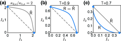
Appendix D Two-mode transducer with asymmetric loss rates
In the main text, we studied two-mode quantum transducer with symmetric loss rates. Here we generalize the discussion to asymmetric loss rates. The scattering matrix now is given by Eq. (39) for , instead of Eq. (13) in the main text. Notice that only depends on the ratios between the device parameters since it is invariant under the transformation
| (48) |
For a two-mode transducer, only depends on , for and . Therefore we set the internal loss rates of both modes to be 1 without loss of generality, and only study the ratios between the external and internal loss rates. In practice, the loss rates of two modes may differ by orders of magnitude, but the ratios and are often close Fan et al. (2018); McKenna et al. (2020); Xu et al. (2021).
In Fig. 7(a), we plot the time-sharing rate region for the asymmetric case with , which demonstrates the benefit from the simultaneous duplex transduction with asymmetric loss ratios. The optimal rate region achieved with the two-side reflectionless condition Eq. (47) requires symmetric ratios . Therefore the rate regions with asymmetric loss ratios (Fig. 7(a)) are all subsets of the optimal rate region in Fig. 3(b)iv.
Appendix E encodings
Although we focus on Gaussian encodings throughout the paper, non-Gaussian states such as single photon states may be easier to implement with current technologies. Here we restrict to the simplest non-Gaussian encodings, the encodings, where the rate regions are obtained from the coherent information (Eq. (5)) for all density matrices in the 0 and 1 photon subspace, i.e., .
We calculate the rate regions for the lossless beam splitter channel (Eq. (1)) at different transmission coefficients. The simultaneous duplex transduction outperforms the time-shared unidirectional transduction for large enough (Fig. 7(b)). This makes sense since the lossless beam splitter approaches the ideal SWAP operation as with a square rate region. Interestingly, is discontinuous at both axes for (Fig. 7(c)) while we do not observe any discontinuity at , although both cases have non-zero reflection coefficients .
References
- Kimble (2008) H. J. Kimble, Nature 453, 1023 (2008).
- Lambert et al. (2020) N. J. Lambert, A. Rueda, F. Sedlmeir, and H. G. L. Schwefel, Advanced Quantum Technologies 3, 1900077 (2020).
- Han et al. (2021) X. Han, W. Fu, C.-L. Zou, L. Jiang, and H. X. Tang, Optica 8, 1050 (2021).
- Andrews et al. (2014) R. W. Andrews, R. W. Peterson, T. P. Purdy, K. Cicak, R. W. Simmonds, C. A. Regal, and K. W. Lehnert, Nature Physics 10, 321 (2014).
- Vainsencher et al. (2016) A. Vainsencher, K. J. Satzinger, G. A. Peairs, and A. N. Cleland, Applied Physics Letters 109, 033107 (2016).
- Fan et al. (2018) L. Fan, C.-L. Zou, R. Cheng, X. Guo, X. Han, Z. Gong, S. Wang, and H. X. Tang, Science Advances 4, eaar4994 (2018).
- Rueda et al. (2019) A. Rueda, W. Hease, S. Barzanjeh, and J. M. Fink, npj Quantum Information 5, 1 (2019).
- Jiang et al. (2020) W. Jiang, C. J. Sarabalis, Y. D. Dahmani, R. N. Patel, F. M. Mayor, T. P. McKenna, R. Van Laer, and A. H. Safavi-Naeini, Nature Communications 11, 1166 (2020).
- Mirhosseini et al. (2020) M. Mirhosseini, A. Sipahigil, M. Kalaee, and O. Painter, Nature 588, 599 (2020).
- McKenna et al. (2020) T. P. McKenna, J. D. Witmer, R. N. Patel, W. Jiang, R. V. Laer, P. Arrangoiz-Arriola, E. A. Wollack, J. F. Herrmann, and A. H. Safavi-Naeini, Optica 7, 1737 (2020).
- Xu et al. (2021) Y. Xu, A. A. Sayem, L. Fan, C.-L. Zou, S. Wang, R. Cheng, W. Fu, L. Yang, M. Xu, and H. X. Tang, Nature Communications 12, 4453 (2021).
- Tu et al. (2022) H.-T. Tu, K.-Y. Liao, Z.-X. Zhang, X.-H. Liu, S.-Y. Zheng, S.-Z. Yang, X.-D. Zhang, H. Yan, and S.-L. Zhu, Nature Photonics 16, 291 (2022).
- Shen et al. (2022) Z. Shen, G.-T. Xu, M. Zhang, Y.-L. Zhang, Y. Wang, C.-Z. Chai, C.-L. Zou, G.-C. Guo, and C.-H. Dong, Physical Review Letters 129, 243601 (2022).
- Tsang (2010) M. Tsang, Physical Review A 81, 063837 (2010).
- Aspelmeyer et al. (2014) M. Aspelmeyer, T. J. Kippenberg, and F. Marquardt, Reviews of Modern Physics 86, 1391 (2014).
- Stannigel et al. (2010) K. Stannigel, P. Rabl, A. S. Sørensen, P. Zoller, and M. D. Lukin, Physical Review Letters 105, 220501 (2010).
- Safavi-Naeini and Painter (2011) A. H. Safavi-Naeini and O. Painter, New Journal of Physics 13, 013017 (2011).
- Hill et al. (2012) J. T. Hill, A. H. Safavi-Naeini, J. Chan, and O. Painter, Nature Communications 3, 1196 (2012).
- Palomaki et al. (2013) T. A. Palomaki, J. W. Harlow, J. D. Teufel, R. W. Simmonds, and K. W. Lehnert, Nature 495, 210 (2013).
- Lecocq et al. (2016) F. Lecocq, J. B. Clark, R. W. Simmonds, J. Aumentado, and J. D. Teufel, Physical Review Letters 116, 043601 (2016).
- Zhang et al. (2014) X. Zhang, C.-L. Zou, L. Jiang, and H. X. Tang, Physical Review Letters 113, 156401 (2014).
- Tabuchi et al. (2015) Y. Tabuchi, S. Ishino, A. Noguchi, T. Ishikawa, R. Yamazaki, K. Usami, and Y. Nakamura, Science 349, 405 (2015).
- Zhang et al. (2018) M. Zhang, C.-L. Zou, and L. Jiang, Physical Review Letters 120, 020502 (2018).
- Wang et al. (2022) C.-H. Wang, F. Li, and L. Jiang, Nature Communications 13, 6698 (2022).
- Note (1) Previous works on “bidirectional conversion” Andrews et al. (2014); Vainsencher et al. (2016); Jiang et al. (2020); Xu et al. (2021) measures the two unidirectional transduction channels separately on a single device, while the duplex quantum transduction we consider here is more general.
- Fawzi et al. (2012) O. Fawzi, P. Hayden, I. Savov, P. Sen, and M. M. Wilde, IEEE Transactions on Information Theory 58, 3670 (2012).
- Sen (2012) P. Sen, in 2012 IEEE International Symposium on Information Theory Proceedings (2012) pp. 736–740.
- Das et al. (2021) S. Das, S. Bäuml, M. Winczewski, and K. Horodecki, Physical Review X 11, 041016 (2021).
- Bennett et al. (2003) C. Bennett, A. Harrow, D. Leung, and J. Smolin, IEEE Transactions on Information Theory 49, 1895 (2003).
- Childs et al. (2006) A. M. Childs, D. W. Leung, and H.-K. Lo, International Journal of Quantum Information 04, 63 (2006), arxiv:quant-ph/0506039 .
- Shi et al. (2021) H. Shi, M.-H. Hsieh, S. Guha, Z. Zhang, and Q. Zhuang, npj Quantum Information 7, 1 (2021).
- Pant et al. (2019) M. Pant, H. Krovi, D. Towsley, L. Tassiulas, L. Jiang, P. Basu, D. Englund, and S. Guha, npj Quantum Information 5, 1 (2019).
- Shi and Qian (2020) S. Shi and C. Qian, in Proceedings of the Annual Conference of the ACM Special Interest Group on Data Communication on the Applications, Technologies, Architectures, and Protocols for Computer Communication, SIGCOMM ’20 (Association for Computing Machinery, New York, NY, USA, 2020) pp. 62–75.
- Vardoyan et al. (2021) G. Vardoyan, S. Guha, P. Nain, and D. Towsley, ACM SIGMETRICS Performance Evaluation Review 48, 45 (2021).
- Dai et al. (2022) W. Dai, A. Rinaldi, and D. Towsley, in 2022 IEEE International Conference on Quantum Computing and Engineering (QCE) (2022) pp. 389–399.
- Wilde (2013) M. M. Wilde, Quantum Information Theory (Cambridge University Press, Cambridge, 2013).
- Schumacher and Nielsen (1996) B. Schumacher and M. A. Nielsen, Physical Review A 54, 2629 (1996).
- Lloyd (1997) S. Lloyd, Physical Review A 55, 1613 (1997).
- Devetak (2005) I. Devetak, IEEE Transactions on Information Theory 51, 44 (2005).
- Weedbrook et al. (2012) C. Weedbrook, S. Pirandola, R. García-Patrón, N. J. Cerf, T. C. Ralph, J. H. Shapiro, and S. Lloyd, Reviews of Modern Physics 84, 621 (2012).
- Holevo and Werner (2001) A. S. Holevo and R. F. Werner, Physical Review A 63, 032312 (2001).
- Rosati et al. (2018) M. Rosati, A. Mari, and V. Giovannetti, Nature Communications 9, 4339 (2018).
- Sharma et al. (2018) K. Sharma, M. M. Wilde, S. Adhikari, and M. Takeoka, New Journal of Physics 20, 063025 (2018).
- Noh et al. (2019) K. Noh, V. V. Albert, and L. Jiang, IEEE Transactions on Information Theory 65, 2563 (2019).
- Zhong et al. (2020a) C. Zhong, Z. Wang, C. Zou, M. Zhang, X. Han, W. Fu, M. Xu, S. Shankar, M. H. Devoret, H. X. Tang, and L. Jiang, Physical Review Letters 124, 010511 (2020a).
- Zhong et al. (2020b) C. Zhong, X. Han, H. X. Tang, and L. Jiang, Physical Review A 101, 032345 (2020b).
- Wu et al. (2021) J. Wu, C. Cui, L. Fan, and Q. Zhuang, Physical Review Applied 16, 064044 (2021).
- Lau and Clerk (2019) H.-K. Lau and A. A. Clerk, npj Quantum Information 5, 1 (2019).
- Zhang et al. (2022) M. Zhang, S. Chowdhury, and L. Jiang, npj Quantum Information 8, 1 (2022).
- Zeuthen et al. (2020) E. Zeuthen, A. Schliesser, A. S. Sørensen, and J. M. Taylor, Quantum Science and Technology 5, 034009 (2020).
- De Berg et al. (2008) M. De Berg, O. Cheong, M. Van Kreveld, and M. Overmars, Computational Geometry: Algorithms and Applications (Springer, Berlin, Heidelberg, 2008).
- Siddiqui and Wilde (2022) A. U. Siddiqui and M. M. Wilde, “Quantifying the performance of bidirectional quantum teleportation,” (2022), arxiv:2010.07905 [quant-ph] .
- Note (2) LOCC-assisted capacity is also known as “two-way capacity”, but we avoid the term “two-way” to prevent any confusion with “duplex” quantum transduction.
- Bennett et al. (1997) C. H. Bennett, D. P. DiVincenzo, and J. A. Smolin, Physical Review Letters 78, 3217 (1997).
- García-Patrón et al. (2009) R. García-Patrón, S. Pirandola, S. Lloyd, and J. H. Shapiro, Physical Review Letters 102, 210501 (2009).
- Pirandola et al. (2017) S. Pirandola, R. Laurenza, C. Ottaviani, and L. Banchi, Nature Communications 8, 15043 (2017).
- Ding et al. (2023) D. Ding, S. Khatri, Y. Quek, P. W. Shor, X. Wang, and M. M. Wilde, IEEE Transactions on Information Theory 69, 3034 (2023).
- Bäuml et al. (2018) S. Bäuml, S. Das, and M. M. Wilde, Physical Review Letters 121, 250504 (2018).
- Das et al. (2020) S. Das, S. Bäuml, and M. M. Wilde, Physical Review A 101, 012344 (2020).