Optimization of the Shape of a Hydrokinetic Turbine’s Draft Tube and Hub Assembly Using Design-by-Morphing with Bayesian Optimization
Abstract
Finding the optimal design of a hydrodynamic or aerodynamic surface is often impossible due to the expense of evaluating the cost functions (say, with computational fluid dynamics) needed to determine the performances of the flows that the surface controls. In addition, inherent limitations of the design space itself due to imposed geometric constraints, conventional parameterization methods, and user bias can restrict all of the designs within a chosen design space regardless of whether traditional optimization methods or newer, data-driven design algorithms with machine learning are used to search the design space. We present a 2-pronged attack to address these difficulties: we propose (1) a methodology to create the design space using morphing that we call Design-by-Morphing (DbM); and (2) an optimization algorithm to search that space that uses a novel Bayesian Optimization (BO) strategy that we call Mixed variable, Multi-Objective Bayesian Optimization (MixMOBO). We apply this shape optimization strategy to maximize the power output of a hydrokinetic turbine. Applying these two strategies in tandem, we demonstrate that we can create a novel, geometrically-unconstrained, design space of a draft tube and hub shape and then optimize them simultaneously with a minimum number of cost function calls. Our framework is versatile and can be applied to the shape optimization of a variety of fluid problems.
keywords:
Draft-Tubes , Hydro-Kinetic Turbines , Design-by-Morphing , Shape Optimization , CFD , Bayesian optimization , MixMOBO , HedgeMO[inst1]organization=Mechanical Engineering Department, University of California, Berkeley,addressline=6116 Etcheverry Hall, city=Berkeley, postcode=94720-1740, state=California, country=U.S.A.
1 Introduction
1.1 Motivation and Background
Renewable energy is fundamental to meeting our energy demands in a sustainable fashion. Although there exist several renewable sources for clean energy (wind, wave, solar, etc.), hydroelectric power is perhaps the most pertinent as a viable replacement for petroleum, natural gas and other fossil fuels. In fact, hydropower was one of the largest renewable energy sources in the United States in 2021 [1]. As such, it is important to consider ways in which the hydroelectric power plant (HEPP) can be more efficient, and thereby more cost-effective.
The relative size of HEPP’s is usually classified by the amount of power they generate. Although there exists no unique definition of “small” hydropower, it is often accepted as a generating capacity at or below 10 megawatt electrical (MWe) [2]. The demand for “small” hydropower is steadily increasing [3] despite concerns about its potential adverse environmental impacts (but impact studies and how the impacts scale with the size of the hydropower plant remain controversial [4, 5]). Currently, there are numerous undeveloped sites across the globe that have large potentials for efficient and sustained power generation via small hydropower [6]. The sites with the most potential and that are easiest to exploit are those with low-impact stream-reaches, existing non-powered dams, and sites with existing conduits [2]. Motivated by this potential for inexpensive and sustainable energy, we propose here a new methodology for the design of some of the parts of a small hydrokinetic turbine. As a specific demonstration of our methodology, we provide a new, more efficient design of the draft tube and hub assembly of a small, low-head Kaplan turbine.
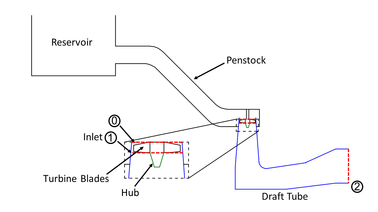
The turbine component of the HEPP works by converting the potential and kinetic energy of the water entering the turbine into mechanical work, and then producing electricity via a generator [7]. As one of the oldest and largest sources of renewable energy, there exists a wide variety of hydrokinetic turbines, but a concept common to all of them is the dynamic pressure or hydraulic head (where is the static pressure, the density and the velocity) of the water entering the turbine. Using Bernoulli’s principle (see 2) we can relate this head to the amount of power an ideal turbine can produce and the physical properties of the hydropower system such as the relative heights of the dam, penstock, and tail water discharge [8]. For high head ranges, impulse turbines (e.g., Pelton) exploit only the velocity of the fluid across the runner (see Fig. 1) to create the mechanical of the turbine blade; whereas in medium and low head ranges, reaction turbines (e.g., Francis and, with later developments for low head applications, Kaplan) exploit both the fluid’s velocity and the fluid pressure or enthalpy across the runner. It is the conversion of enthalpy that allows the draft tube and hub assembly to enhance the performance of a reaction turbine [9, 10]. The draft tube and hub assembly make up only part of the overall hydropower system’s performance, but they are most important for low-head turbines, which we consider here to be those under 20 m.
The draft tube is a diffuser, or several diffusers joined together, that sits beneath the runner of the turbine and directs the flow downstream of the turbine blades to the tailwater pool. It therefore has a large role in determining the dimensions of the lower section of the power plant [11]. The draft tube increase the efficiency of the turbine by adjusting the dynamic pressure such that the static pressure just downstream of the turbine blade is decreased. The adjustment is done by decelerating the velocity of the fluid passing through the draft tube, and it is this property (hereafter referred to as the “pressure recovery”) that affects the power-generating capacity of Kaplan and other reaction turbines [12, 13].
The hub is a conically shaped part that extends just past the inlet of the draft tube, centered about the axis turbine’s of rotation and connecting its blades. Water flows into the draft tube through an annular-shaped region between the hub and the draft tube wall. The hub rotates with the same angular velocity as the turbine blade, while the outer boundary of the draft tube is non-rotating. (See Fig. 1.) It is important to optimize the hub because it modifies the inlet flow to the draft tube, and therefore has a large effect on the pressure recovery.
Poorly designed parts of the draft tube or hub can significantly decrease a turbine’s efficiency by exacerbating turbulence and increasing friction losses. For example, the draft tube’s elbow (Fig.1), which is necessary for redirecting the tailwater flow, can promote flow separation due to excessive centrifugal force at its inner radius. Similarly, a poorly designed hub can allow the swirl flow at the inlet due to the turbine blades create instabilities in the flow that lead to noise, vibration (prompting failure due to fatigue), and even the reversal of flow through the center of the draft tube (causing sudden changes in power output of the turbine) [14]. A well-designed hub can help prevent these problems, and, in addition, allow a larger opening angle of the diffuser (and therefore higher pressure recovery). As such, we not only optimize the draft tube, but also the hub, which is usually neglected in prior optimization studies [15, 16, 17].
Much of the optimization effort of Kaplan draft tubes in recent years was focused on improving the sharp-heeled elbow draft tube [17]. This shape was first installed in 1949 at the Hölleforsen Hydro Power Station in Vattenfall, northern Sweden, utilising a 25m head and with a power generating capacity of 150 MWe [18]. Gubin [17] and Dahlbäck [19] independently argued that this draft tube shape needed improvement, and subsequently there have been many proposed design changes. Marjavaara and Lundström [20] and Marjavaara [15] use a Response Surface Method (RSM) surrogate modeling strategy, as well as a commercial CFD code (ANSYS CFX4.4) to create new designs with different parametrizations (circular and elliptical, respectively) of the elbow section. More recent improvements include those of Daniels et al. [21, 22] who use multi-objective Bayesian optimization to maximize pressure recovery using a series of subdividing curves, optimizing over the inflow cone, outer-heel, and secondary straight diffuser. Other improved designs focus on the optimization of the draft tube for low-head applications while retaining the sharp-heel shape [23, 24].
1.2 Design-by-Morphing
Design search space creation or parametrization is an integral part of any shape optimization process. Parameterization determines both the design space and the complexity of the optimization problem. A desirable parameterization technique must cover a wide design space within a limited number of design parameters[25, 26, 27], necessary during the early design stage when minimum geometric constraints are placed and radical changes during the optimization process are required.
For a set number of parameters, parametrization techniques are judged on the different fidelity and ranges of control they offer [28, 27, 25]. Discrete methods [29], where design parameters are exactly the discrete surface points that define the airfoil shapes. The displacement of each point can be adjusted [30], and very fine local control can be achieved. However, to describe a shape accurately and with high fidelity, a large number of surface points are needed, which increases the number of parameters of the optimization problem. To accommodate the large number of design variables, gradient-based method are usually used to guide the optimization which can easily get stuck at a local optimum.
High-fidelity features can be captured by B-splines [31, 32], and nonuniform rational B-spline (NURBS) [33] which form curves by connecting low-order Bézier segments defined by the control points. The fidelity of shape representation with these techniques depend on the number of parameters used for curve definition, increasing the computational complexity. To reduce the number of the design parameters, the control points can be grouped together, free-form deformation (FFD) method [34, 35]. Other techniques include spectral representation techniques which use some basis functions or modes, such as proper orthogonal decomposition (POD) [36, 37], Hicks-Henne’s approach [38], and class/shape function transformation (CST) method [39, 40].
To address the design challenges for improved hydrodynamic and aerodynamic surfaces, we introduced a new framework, Design-by-Morphing (DbM), for creating a design space that is versatile enough to include old and new designs and that is sufficiently free of human bias to produce a radical and counter-intuitive design search space. The strategy cannot be called fully free from designer bias due to the choice of baseline shapes by designer, but the negative weights and radical baseline shapes, described later, minimize this effect. DbM uses the shape space as the basis for the parametrization scheme, thus allowing infinite fidelity without increasing the design space parameters for any shape, since it is the weight on the shape itself that is optimized. This is not possible with any conventional scheme discussed above and DbM has been shown to reproduce the entire UIUC database to very fidelity using just 25 parameters in [41]. DbM was first used by Oh et al. [42] and later used in other optimization problems [41, 43]. An -dimensional design space for a shape is created by choosing baseline shapes. The shape within our design space is specified by the choice of the weights of these baselines from which the design is morphed. The bounds of the weights are sufficiently large that the morphed shapes can be not only interpolations among the shapes, but also extrapolations. Furthermore, any of the weights can be negative so that features of poorly performing baseline shapes can either be suppressed or entirely avoided. Negative weights and large positive weights allow for unintuitive shapes and for extrapolations. Many design techniques only allow for small departures from existing designs [44] or allow only local changes at one or a few specific locations, rather than global changes to the overall shape [45, 46]. This is especially problematic with most methods that use control points. CAD, and/or NURBS. Generally, methods with parametric control [28, 45, 47, 48, 49] and the adjoint method [44, 46, 50] limit the amount of change that can be made to a design so that radical new designs are not possible. DbM also allows a more extensive design space where both spatially local and global changes can be made to the design, and those changes can be subtle and/or radical [41]. This allows us to find an optimum which may be a completely new, unconventional shape [42].
1.3 Improved Bayesian Optimization
Once a design space is chosen, many engineering optimization problems require the repeated numerical (or laboratory) evaluation of an expensive multi-modal black-box function to determine the performance or cost of a particular design. In optimizations of a surface that interacts with a fluid, generally the fluid flow must be computed with an expensive Computational Fluid Dynamics (CFD) program to determine the quantitative performance of each candidate design. Those quantitative results are then fed into an optimizing algorithm to determine the best performing design. The expense of computing the performance function with CFD makes many optimization problems intractable. Furthermore, the highly nonlinear behaviour of fluid flows often leads to a design space where the performance function has many local maxima, and it is difficult for the search algorithm to find the global maximum.
Optimizing draft tubes is an example of a search requiring an expensive multi-modal, black-box, performance function because the efficiency and pressure recovery of each candidate draft tube must be computed with CFD. Gradient based optimization techniques are unsuitable for multi-modal optimization since they get stuck in local optima and might require a number of function calls to either multi-start or get out of the local optimum. Global optimization schemes, such as evolutionary algorithm on the other hand require a large number of function calls to reach a global optimum, making them unsuitable for expensive black-box functions. Compared to Bayesian optimization, a genetic algorithm requires at least two orders of magnitude greater number of function calls to find the global optimum [51]. Bayesian Optimization (BO) is an efficient search method for this type of optimization because it requires far fewer evaluations of the performance function to find an optimum than most other optimization algorithms [52, 53]. BO techniques have been successful in the design of architected meta-materials [54, 55, 56, 57, 58, 59], hyper-parameter tuning for machine learning algorithms [60, 61, 62], drug design [63, 64], and controller sensor placement [65]. In this study, we use an improvement that we made to BO, that we call Mixed-variable Multi-Objective Bayesian Optimization (MixMOBO) [51]. Previously, we used MixMOBO to design an architected meta-material that has maximum strain-energy density [59].
2 Preliminaries
Any kinetic energy or potential energy that is not converted into mechanical energy of the turbine shaft (and then into electrical energy) is discarded (i.e., wasted) when it leaves the turbine blades. A well-designed draft tube minimizes the wasted energy by converting dynamic head into static head. The schematic of a hydrokinetic turbine assembly is shown in Figure 1. The overall drop in pressure across the turbine blade is , where is the average fluid pressure just upstream of the turbine blade and is assumed to be fixed and independent of the designs of the hub and draft tube. is the average fluid pressure just downstream of the turbine blade, which is dependent on the designs of the hub and draft, and, in general, must be computed numerically and cannot be estimated using control volume analysis or a Bernoulli equation. However, control volume analysis does allow us to estimate the theoretically available power, , that can drive the turbine blade and produce electricity. It is
| (1) |
where are the cross-sectional areas of the flow upstream and downstream of the turbine blade (where the subscripts refer to the location in Fig. 1) and are the characteristic velocities at these same locations.111Although can be thought of as an average streamwise velocity of the fluid upstream of the turbine blades, the amount of power that the blades can extract depends on the detailed flow interaction of the fluid velocity with the blade, which among other things depends on the swirl of the upstream velocity. Therefore, we leave the definition of this ‘characteristic’ velocity purposefully undefined. We assume that along with , and are fixed, given parameters, and are not affected by the hub and draft tube designs. The goal of a well-designed hub assembly and draft tube is to maximize .
Traditionally, [11, 13, 66], the mean pressure recovery is defined as and is the performance function used to the power output . We define the dimensionless mean pressure recovery coefficient as:
| (2) |
where is the density of the fluid, and are the average pressures, averaged over their respective cross-sections, and the subscripts refer to the location in Fig. 1. Using this definition and eq. (1), we see that and are related by
| (3) |
Because is positive (and because , , , , , and are assumed to be fixed, and independent of the designs of the hub and draft tube), maximizing and maximizing are equivalent. We therefore have chosen to be the performance function that is maximized in this study.
Note that in order to prevent back flow without a draft tube, would need to be greater than or equal to the given reference or gauge pressure . Because is assumed to be given (and the same value with or without a draft tube), the maximum value of without a draft tube would be constrained by
| (4) |
The draft tube allows , and therefore allows an extra amount of power, , to be generated. Note that because , , and are assumed to be fixed, maximizing minimizes . Also note that because the fluid must be discharged from the draft tube at () with a finite velocity, and therefore the discharged fluid must necessarily contain some kinetic energy that cannot be recovered or converted into shaft mechanical energy, can never sufficiently maximized, and never sufficiently minimized (even in the inviscid case) to make the generating system 100% efficient [7, 8, 9].
3 Methodology
An overview of our procedure is demonstrated in the schematic in Fig. 2. Our method starts with five different draft tube and two different hub baseline shapes to create the DbM search space. This search space is then initially sampled randomly for 50 data points. This data was then used to determine the next epoch or batch of designs or test points to evaluate using the MixMOBO algorithm. Each batch is a set of 5 data points or designs. As each new batch of designs is evaluated, their ’s are added to the data base that MixMOBO uses to compute the next batch of designs to evaluate.This procedure continues until the evaluation budget is reached.

3.1 Baseline Shapes
The design space is created from five baseline draft tube shapes and two baseline hub shapes. The shapes are morphed with the weights chosen by MixMOBO to create a new draft tube and hub shape. These baselines are shown in Figure 2. The five baseline draft tube shapes are homeomorphic to each other as are the two baseline hub shapes. Some of the baselines that we chose were used previously in literature so that we were able to exploit any inherent advantageous features they might have, while other baselines were chosen to have non-intuitive features that would lead to radical designs, rather than incremental improvements. In the past, the fundamental design features of the Kaplan draft tube were formed through experimental observation and quasi-empirical formulae derived from geometries already installed and in use in HEPPs [21]. The works of Gubin [17], Cervantes [11], Mulu [67] and Nilsson et. al. [14] [68]) provide insights into draft tube geometries.
Our first baseline shape for the draft tube is the sharp heel draft tube, which has been the focus of extensive optimization attempts. It is also the subject of extensive experimental and numerical studies, the majority of which were completed through the European Research Community On Flow, Turbulence And Combustion (ERCOFTAC) Turbine-99 Workshop series [69, 70, 66]. For this reason, this shape also provides excellent validation of our CFD setup.
The second and third baseline draft tube shapes are based on designs cited by Gubin [17] and are particularly well-suited to low-head applications (i.e., for Kaplan turbines). The fourth and fifth baseline tube shapes were both devised in order to create features which would expand the design space. These shapes were generated by taking the average shape of the first three baseline shapes and then adding radically different features such as a rounded outlet and a circular diffuser shape. The addition of these baseline shape can be thought of in a similar manner to adding mutation within a generation in genetic algorithms. All the baseline draft tubes have the same shape at their inlets, and in all cases the planes containing inlet and outlet are perpendicular to each other.
Both baseline hubs have the same radius at the inlet, the same radius at the end of the hub, and the same length. The first baseline hub shape is based on one currently used in a Kaplan turbine [67, 71]. The second baseline hub is a cone shape, and which was historically used in a wide variety of low to medium head reaction turbines [17]. Morphing these two hubs allows for a variation in the inlet geometry, which in turn modifies the flow profile near the inlet and therefore the pressure recovery. The baseline hub shapes are shown in Figure 2.
3.2 Design-By-Morphing
Design-by-Morphing (DbM) works by creating a one-to-one correspondence between the set of baseline shapes. The shapes are then “morphed” i.e. linearly combined together using “weights”. These weights are the independent parameters that form the search space for optimizing the shape. DbM requires that the set of shapes be homeomorphic or topologically equivalent so that a one-to-one correspondence can be created between the surface elements. This one-to-one correspondence is created by defining a collocation strategy for the baseline shapes that ensures all constraints for our design are fulfilled (for example inlet and outlet orientation) even if individual shapes are radically different from each other.
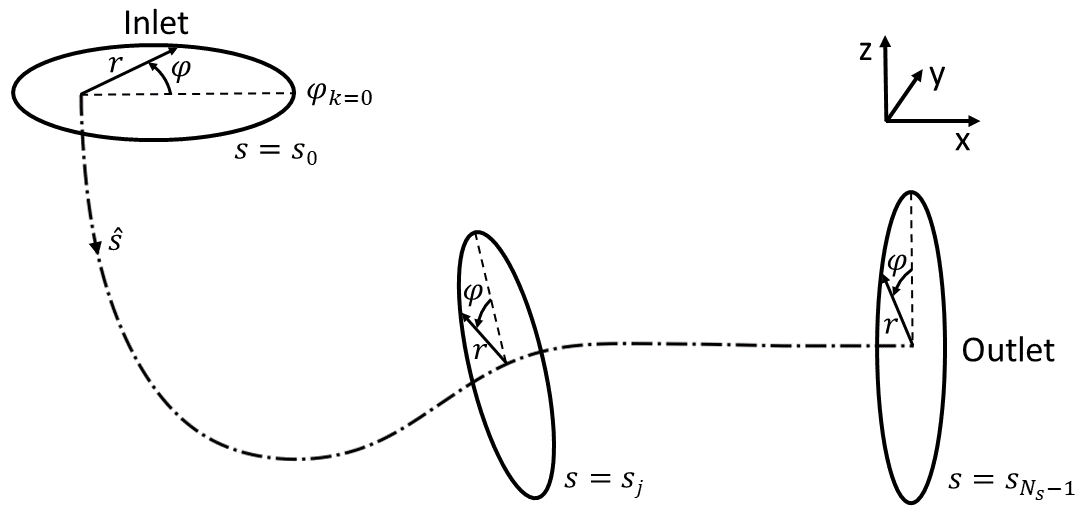
For the draft tube baseline shapes (shown in Figs. 3 and 4), the inlet is constrained to a plane parallel to the horizontal (-) plane and the outlet is constrained to a plane parallel to the vertical (-) plane for all the baseline shapes. Note that this ensures that all the morphed shape inlets and outlets are similarly constrained i.e. inlets are in the same horizontal plane and the outlets are in the same vertical plane. Fig 3 explains how we construct a single coordinate system for all of the baseline and morphed draft tubes that is mapped from the cylindrical coordinates . The axis is mapped to the origin curve in the figure with with arc length and local unit vector . The boundary of the draft tube is defined by its intersections with each of the perpendicular planes shown in Fig. 3. Within each perpendicular plane, the intersection of the plane with the draft tube boundary is defined by the closed curve , the radial distance of the draft tube boundary from the origin curve in the perpendicular plane. We note here that, because the same origin line is used for all of the baseline shapes, the start and end points of the origin line are always constrained to the same location in the inlet and outlet planes. The draft tube shape, however, changes around the origin line, meaning that the average path length for a fluid particle to travel from inlet to outlet, can vary for each draft tube.
In each of the perpendiclar planes, we discretize into equally-spaced collocation angles with , with and . The radius of the draft tube as a function of the arc length and polar angle is completely defined by the radial location matrix , with , and . Note that the perpendicular planes and the collocation angles are the same for all of the the baseline and the morphed draft tubes.
For hub shapes, the same collocation strategy is used as we used for the draft tube shapes, with the origin curve of the hubs passing through the center of both of the baseline hubs because the baseline hub are axi-symmetric.
After morphing, each morphed radial matrix can be projected back into a 3-D shape as in Figure 4.

Because all of the five baseline draft tube shapes are homeomorphic, they can easily be combined into a new morphed shape, given by , once the weights , of each baseline are chosen (see Fig. 4):
| (5) |
Note that negatives weights and weights greater than unity allow for extrapolations; negative weights also allow us to “avoid” some baselines. This means that the only existing constraints are those imposed by choosing the baselines shapes themselves. That said, the lack of CAD parameterization means that DbM may produce non-physical, self-intersecting shapes when negative weights are applied. If the morphed shape is not physical because it has intersecting radial boundaries, we set the pressure recovery function of that morphed draft tube function to be zero so that the optimization method avoids that region of design space. For draft tube optimization, we limit the allowable range of the weights of each of the draft tubes such that: .
The morphed shape of the hub is given by an equation similar to eq. (5), but the sum is over only 2 baseline radii. We denote the weights for hubs with to differentiate it from the draft tube weights. Furthermore, the sum weight for the second hub baseline is constrained by , and for the morphed hub shape, . Due to the fact that sums of the weights of the draft tube baseline shapes and of the hub baseline shapes are fixed, there are only 6 degrees of freedom in choosing the values of the weights of the baseline shapes, so our design space has 6 dimensions.
3.3 CFD Setup and Validation
The coefficient of pressure recovery of each morphed draft tube shape that is physically allowable is determined with CFD. We validated the CFD code by comparing our simulations of the sharp heel draft tube with previously published results. In order to compute the flow in a morphed hub and draft tube shape, a mesh of that shape is created from a surface point cloud of the shape using Gmsh [72]. The average statistics of a typical mesh is given in Table 1, where D is the inlet diameter. The software used is OpenFOAM, and the solver used is pimpleFoam.
| Max Cell Size / D | 0.638 |
| Number of Elements | 7.9e+05 |
| Number of Nodes | 1.3e+05 |
| Meshing Algorithm | Delaunay (3D) |
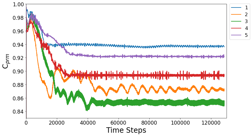
For turbulence modeling, we use the - turbulence model. This choice was made based on its success in previous draft tube studies [13, 73]. Based on the kinematic viscosity of water, the distance between the outer edge of the hub and the inlet wall, and the average streamwise velocity at the inlet, the Reynolds number is 5.56e+05, and based on the azimuthal velocity of the hub, it is 9.48e+05. No-slip conditions are applied at the rotating, inner hub wall () and at the non-rotating draft tube boundary.222The optimization studies in the past for draft tubes [23, 24], did not consider a rotating hub inlet condition, which makes the CFD boundary conditions less close to the actual operating or experimental conditions The inlet velocity is axisymmetric with non-zero values of the azimuthal, radial, and streamwise components. Our CFD simulations use the experimentally measured inlet velocities found by Engström et al. [70]. The outlet pressure is the pressure at location in Fig. 1, and is fixed gauge pressure, but the pressure at the inlet, needed to determine the , is computed by the CFD code as a function of , , and time. We run the CFD for 128,571 time steps for each morphed hub/draft tube shape. Our choice of the number of time steps is based on how long it takes the solution to reach a statistical steady state – see Fig. 5. Note that , given by eq. (2), is not determined at a single time step, but rather it is averaged over the final 28,500 time steps of the computation (and note that as shown in Fig. 5, the solution has converged to a statistically-steady equilibrium during those final time steps). The time step was chosen to be , where is the outer diameter of the hub and is the average streamwise inlet velocity. This time step was chosen based on a time resolution study (see below).
The CFD is validated in two ways. The first compares our CFD-computed pressures with the experimentally-measured values along the top and bottom center lines of the baseline 1, Sharp-Heel, draft tube. The second uses baseline 1 to test the convergence of the CFD code by refining the numerical time step and grid size. We note here that the experimental studies did not provide the values, thus no comparison could be made.
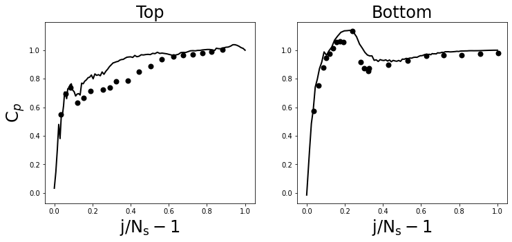
The local pressure recovery along the top and bottom lines of the first baseline shape (i.e., the sharp heel draft tube) is shown (and defined) in Figure 6. The figure compares our numerically-computed local pressure recovery values to the experimentally-measured values [70]. Figures similar to Fig. 6 appear throughout the ERCOFTAC Turbine-99 Workshop series, and the deviation between our CFD and experimental values are consistent with the previous numerical studies.
The second way we validated our use of our OpenFoam code and gridding scheme was by time step and mesh refinement. We chose our time step size by decreasing its value in the CFD code until the late time-averaged values of the sharp heel draft tube with the first hub baseline shape changed by less than . In particular, once we set the value of the time step as , we repeated the calculation of the local pressure recovery for both the top and bottom as a function of as defined in Fig. 6 – once with a time step greater than that used in the figure and once with it lower. Plots of these new curves computed with these time steps are indistinguishable from the curves (error less than 0.5%) shown in Fig. 6 (at the resolution at which we created the figure), validating that our time step is sufficiently small. We determined the size of the spatial resolution of the grid for the CFD in a similar manner: we decreased the grid size (or equivalently, increased the square of the number of grid points) until the late time-averaged values values of the sharp heel draft tube changed by less than . We also recomputed the two curves of the in Fig. 6 with a spatial resolution of the spatial gridding mesh with a size that was greater than that used in the figure and once with it lower. Again, we found that the plots of these new curves computed with these grids are indistinguishable (error less than 0.5%) from the curves shown in Fig. 6, validating that our grid is sufficiently fine.
It is important to note that Fig. 5 shows that it takes more than 50,000 time steps for our numerically-computed to reach a statistical equilibrium. The 50,000 time steps corresponds to a time that is approximately equal to 10 “advective times”, where the latter is the streamwise length of the draft tube divided by the average streamwise velocity at the inlet . Previous numerical studies of draft tubes were often validated by comparing the numerically-computed local pressure recovery at the bottom or top of the draft tube with the experimentally measured values. However, in many of those studies the codes were run for only one advective time (5000 of our time steps) before the pressure recovery factor was evaluated [70]. Figure 5 clearly shows that although that time be sufficient to numerically capture the final statistically steady state of , it is insufficient for the full flow and to have come to a statistical steady state.
3.4 Bayesian Optimization
In our previous work, we developed a Mixed-variable, Multi-Objective Bayesian Optimization (MixMOBO) algorithm [51], a framework for optimizing mixed-variable, multi-objective problems with noisy black-box function using parallel batch updates of the data set, that is, letting the acquisition function pick several points to evaluate at each iteration to allow their CFD evaluations to be carried out in parallel. MixMOBO was proven to be more efficient in terms of number of black-box function evaluations compared to other algorithms in small data settings. In our previous studies, we used MixMOBO to design a microlattice structure with the objective of maximizing its strain-energy density [59]. We are also applying MixMOBO for the optimization of vertical axis wind turbines [43].
Our current study adapts the generalized MixMOBO algorithm for the specific case of 6 continuous variables with parallel batch updates using the HedgeMO algorithm [51]. Our HedgeMO strategy uses the Upper Confidence Bound, Expected Improvement, Probability of Improvement, and Stochastic Monte-Carlo [52, 51] acquisition functions. We apply our Bayesian optimization algorithm in tandem with DbM here for the shape optimization of a draft tube/hub. This section details our adaptation of the MixMOBO algorithm for our current study.
The search in our 6-dimensional design space (consisting of the 5 weights of the baseline draft tubes and the 1 independent weight of the two baseline hubs) for the draft tube/hub design with the maximum is an example of an optimization problem that can generically be posed as:
| (6) |
where is the objective to be maximized (in this case ), and is a -dimensional (in this case 6-dimensional) variable vector, defined over a bounded set (in this case, the weights of the baselines). For many practical engineering problems, is expensive to evaluate (as is the case here, which requires repeated CFD evaluations of a complex draft tube designs). In such cases, a Bayesian optimization algorithm is often the best choice [52]. Bayesian optimization is a sequential optimization technique, specifically designed to find the optimal solution of a noisy black-box function with the fewest possible evaluations or function calls to . At every iteration of the algorithm, a surrogate model , usually a Gaussian process (GP), is fit over the data set .
| (7) |
Here is the total number of evaluated points (in this case, morphed draft tube/hub designs) and is the vector of continuous variable vector.
The MixMOBO algorithm is agnostic to the choice of kernel function. For our current study, we use a simple modified squared exponential kernel due to its good performance for continuous variable problems:
| (8) |
where is a vector containing all the hyper-parameters, is the covariance hyper-parameter matrix and is the vector of covariance lengths and distance between the variables defined to be their Euclidean distances.
Once the GP surface has been fit, the next query point in the design space that should be chosen to evaluation must explore the space that most probably contains the optimum (e.g., the design with the largest ), and must also try to improve the fit for the next iteration, i.e. choose a region of space where information is sparse. These two determinations are not the same, and the former is called “exploitation” and the latter “exploration”. Bayesian optimization strives to create a balance of exploitation and exploration that continues until there is either evidence that a global optimum has been found or a maximum prescribed number of iterations of the algorithm is reached. An acquisition function, which we represnt here by , determines the next query point (or points) in the design space to be evaluated with (in this case, with the costly CFD), by balancing the competing needs of exploitation and exploration. Once the next query point (or points) has been determined , is evaluated for that point (or points) and is then appended to the data set, . To optimize the exploitation/exploration balance, we use a GA to optimize the acquisition functions, which, although expensive to use on an actual black-box function, is an ideal candidate for optimizing the acquisition function working on the surrogate surface.
MixMOBO uses HedgeMO, a hedging strategy for acquisition functions, as part of its framework. Hedge strategies use a portfolio of acquisition functions, rather than a single acquisition function [74]. HedgeMO also allows parallel ‘-batches’ of query points. The detailed algorithmic flowchart of our adapted MixMOBO algorithm is shown in Algorithm 1. We note that the convergence criterion presented by [74] holds for our portfolio as well.
The process is repeated until the evaluation budget is reached. Our choice for the evaluation budget was based on several optimization experiments on test functions and design spaces, described below, that we believe to be representative of the draft tube/hub optimization. To determine the number of iterations of the Bayesian optimization algorithm, or epochs (where each epoch determines the of 5 morphed draft tube/hub designs in parallel), required to likely find the optimal design within the design space, we carried out optimizations of a suite of test functions with different properties and whose maximum values could be determined analytically. We optimized the Spherical, Rastringin, Syblinski-Tang and Amalgamated functions, all of which are standard functions used to test optimization schemes [75] with the exception of the Amalgmated function, which is novel and created by us to mimic some of the properties of the draft tube/hub design space. The test functions that we used to determine the number of epochs that are needed for MixMOBO to likely find the maximum are defined in Table 3. Similar to the design space of the draft tube/hub, each test function was tested with 6 dimensions.
| Name | Objective Functions | Notes |
|---|---|---|
| Spherical | ||
| Rastringin | ||
| Syblinski-Tang | ||
| Amalgamated |
Figure 7 shows how MixMOBO approaches the global maximum of each of the four test functions as a function of epoch. Two of the four test functions find the global maximum within 75 epochs.
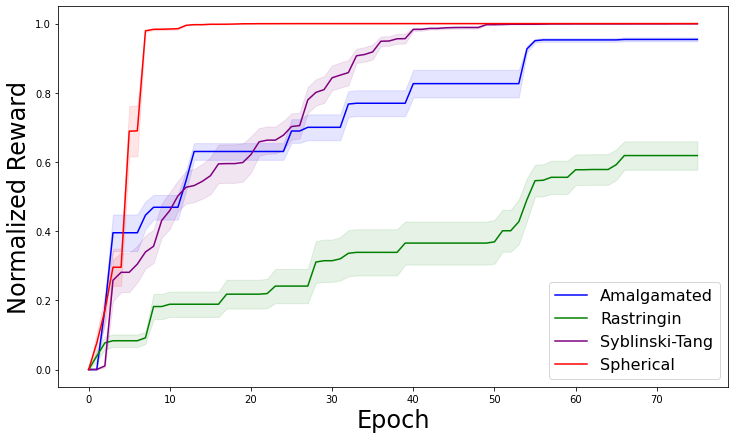
The optimization was terminated after 75 epochs because the test functions reached reasonable convergence, other than Rastringin function, which is know to have a a multitude of local optima, as shown in Fig. 7. We could only afford 75 epochs worth of CFD evaluations of candidate draft tube designs in our computational budget so the evaluations were not carried past 75 epochs. As depicted in our Results, the draft tube optimization converged to the final design in 30 epochs. MixMOBO, like most Bayesian optimization schemes, needs to be initialized with evaluations of random designs. Based on the results shown on Test Functions, we use 50 random evaluations, and 75 epochs with 5 parallel batch evaluations per epoch to optimize our 6-dimensional design space.
4 Results
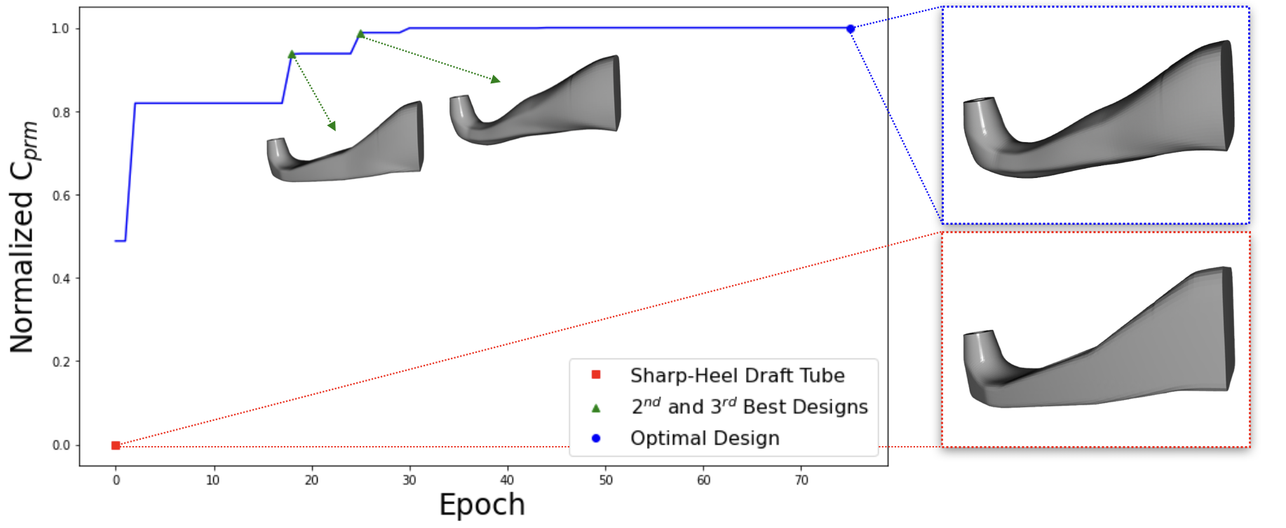
We searched for the morphed draft tube/hub design with the maximum in our 6-dimensional design space using MixMOBO with 50 initial random designs and 75 epochs with 5 design evaluations per epoch. The results our shown in Fig. 8 and Table 4. The Normalized used in the figure is defined as: of Current Epoch’s Optimum of Sharp heel draft tube with the baseline 1 hub of the Optimum design found by MixMOBO of Sharp heel with baseline 1 hub.
We note here that our CFD simulations are run to convergence, as explained in Section 3.3. If we ran our simulations for only one advective time, we would potentially have gotten a higher value, which would not be converged and erroneous, as shown in Fig. 5.
Figure 8 and the Table show that the of the sharp heel draft tube with the baseline hub 1 is significantly lower than the of the best (and second and third best) design found with MixMOBO. In fact, the of the best of the 50 random designs that were used to initialize MixMOBO was better than that of the sharp heel draft tube, which shows the strength of our Design-by-Morphing approach. The sharp heel draft tube had the best (when coupled with hub shape 1) of all the baseline draft tubes. We note that the of the optimal design found by MixMOBO is significantly better than the Sharp-Heel draft tube, which is the draft tube of choice for Kaplan turbines around the world [17].
| Design | Epoch | |||||||
|---|---|---|---|---|---|---|---|---|
| Sharp-Heel | 1 | 0 | 0 | 0 | 0 | 0.5 | ||
| Best | 19 | 0.86 | -0.17 | 0.40 | -0.21 | 0.98 | 0.98 | |
| Best | 26 | 0.88 | -0.24 | 0.26 | -0.17 | 0.99 | 0.92 | |
| Optimal | 30 | 0.90 | -0.14 | 0.22 | -0.25 | 0.99 | 0.99 |
Note that all three of the morphed draft tube/hub designs in Table 4 have at least one negative weight, meaning that they are extrapolations, rather than interpolations of the baseline shapes. Generally, extrapolation is not possible with conventional design techniques. The Design-by-Morphing (DbM) response surface is highly sensitive to any changes in the values of the weights, which makes the DbM design space highly non-convex. We found that with each new epoch, small changes in the weights led to significant changes in the overall shape of the morphed draft tube/hub. This characteristic means that the DbM space needs to optimized with high precision where very small changes in the weights need to be considered. In particular, if we were to consider the value of each weight to be a discrete, rather than a continuous variable, then the design space would need to have a very large number of discrete variables. Since we are treating the weights here as continuous variables, the sensitive dependence of the morphed shape on the weight values means that most conventional optimization schemes, the search may get “stuck” at a local maximum and will fail to find the global maximum. Bayesian Optimization algorithms, including MixMOBO, that are designed to search for the global maximum of , will tend to over-explore the region of the design space around a local maximum. This effect, however, is less pronounced for BO based schemes since they do not depend upon the gradient of the surrogate surfaces. MixMOBO also uses “mutation” to get out of the local maxima. Our numerical experiments with MixMOBO show that it tends to not get stuck at local maxima, and it finds the global maximum [51].
5 Conclusion
We have introduced a novel systematic shape optimization framework using the Design-by-Morphing (DbM) technique with a Mixed-variable Multi-Objective Bayesian Optimization (MixMOBO) algorithm. As a proof-of-concept of this optimization framework, we found the shape of a draft tube/hub for a hydrokinetic turbine such that the coefficient of pressure recovery was maximized. Our Design-by-Morphing (DbM) technique creates novel shapes from interpolations and extrapolations of pre-existing designs and/or new ones, and the shapes we create are free from designer’s biases. Most existing design strategies cannot extrapolate among designs, and this limits their abilities to create radically different designs.
The design space created with the Design-by-Morphing framework was searched by our novel MixBOBO Bayesian Optimization. This search method is especially useful when the property that is being optimized, in this case the , is costly to compute (or find experimentally). In these cases, it is necessary for the search algorithm to find the optimum design with as few evaluations of as possible. Using MixMOBO, we successfully found a design with large (certainly a local maximum in the design space, and possibley the global maximum) with 30 epochs, or 200 evaluations of a design’s .
The draft tube/hub design found here has a significantly better coefficient of mean pressure recovery than the sharp-heel draft tube, which is the most commonly used draft tube for hydrokinetic turbines. More significantly, we have shown that the design framework used here, which can easily be generalized to a number of engineering design optimization problems, with the current study providing a proof-of-concept for our optimization framework. DbM provides a methodology to create a bias and constraint free design space which also allows extrapolation from the existing designs and can yield radical shapes. MixMOBO provides a global optimization strategy to optimize optimize design spaces where evaluating each candidate design is extremely expensive, the design space contains mixed variables and/or multiple objectives, rendering conventional optimization techniques intractable. The framework can be used for optimizing expensive black-box shape optimization problems such as vertical-axis wind turbines [43], high-performance airfoils [41] and architected meta-materials [51].
References
- eia [2022] U.s. energy information administration monthly energy review, december 2021, https://www.eia.gov/totalenergy/data/monthly/archive/00352112.pdf, 2022.
- Curtis et al. [2017] T. Curtis, A. Levine, K. Johnson, State models to incentivize and streamline small hydropower development, National Renewable Energy Laboratory (NREL), U.S. Department of Energy, 2017.
- of Energy [2001] U. S. D. of Energy, Hydropower vision, https://www.energy.gov/sites/default/files/2018/02/f49/Hydropower-Vision-021518.pdf, 2001. Accessed 03-29-2022.
- Bakken et al. [2012] T. H. Bakken, H. Sundt, A. Ruud, A. Harby, Development of small versus large hydropower in norway– comparison of environmental impacts, Energy Procedia 20 (2012) 185–199. URL: https://www.sciencedirect.com/science/article/pii/S1876610212007497. doi:https://doi.org/10.1016/j.egypro.2012.03.019, technoport 2012 - Sharing Possibilities and 2nd Renewable Energy Research Conference (RERC2012).
- Couto BA and Olden [2018] T. Couto BA, J. D. Olden, Global proliferation of small hydropower plants - science and policy, in: Front Ecol Environ, volume 16, 2018, pp. 91–100. doi:https://doi.org/10.1002/fee.1746.
- Hall G. et al. [2006] D. Hall G., K. S. Reeves, J. Brizzee, R. Lee D., G. Carroll R., G. Sommers L., Feasibility assessment of the water energy resources of the united states for new low power and small hydro classes of hydroelectric plants, Idaho National Laboratory, 2006.
- Kaltschmitt et al. [2007] M. Kaltschmitt, W. Streicher, A. Wiese, Renewable Energy: Technology, Environment and Economics, Springer, Berlin, Heidelberg, 2007.
- Mulley [2004] R. Mulley, Flow of Industrial Fluids - Theory and Equations, Taylor & Francis Group, LLC, 2004.
- Warnick et al. [1984] C. C. Warnick, H. A. Mayo, J. L. Carson, L. H. Sheldon, Hydropower Engineering, Prentice-Hall, Inc., 1984.
- Sheldon [1998] L. H. Sheldon, Reviewing the approaches to hydro optimization, Hydro Review 17 (1998) 60–67.
- Cervantes [2003] M. J. Cervantes, Effects of boundary conditions and unsteadiness on draft tube flow, ph.d. thesis, Division of Fluid Mechanics, Luleå University of Technology (2003).
- Krivchenko [1994] G. Krivchenko, Hydraulic Machines: Turbines and Pumps, CRC Press, Inc., 1994.
- Andersson [2009] U. Andersson, An experimental study of the flow in a sharp-heel kaplan draft tube, ph.d. thesis, Division of Fluid Mechanics, Luleå University of Technology (2009).
- Nilsson [2006] H. Nilsson, 3d numerical analysis of the unsteady turbulent swirling flow in a conical diffuser using fluent and openfoam, in: IAHR 2006, 2006.
- Marjavaara [2006] B. D. Marjavaara, Cfd driven optimization of hydraulic turbine draft tubes using surrogate models, Division of Fluid Mechanics, Luleå University of Technology (2006).
- Dahlhaug [1997] O. G. Dahlhaug, A study of swirl flow in draft tubes, Norwegian University of Science and Technology Trondheim, 1997.
- Gubin [1970] M. Gubin, Draft Tubes of Hydro-electric Stations, Energiya Press, Moscow, 1970.
- hol [2022] Hölleforsen - vattenfall ab, https://powerplants.vattenfall.com/holleforsen/, 2022. Accessed: 2022-03-28.
- Dahlbäck [1996] N. Dahlbäck, Redesign of sharp heel draft tube - results from tests in model and prototype, in: E. Cabrera, V. Espert, F. Martínez (Eds.), Proceedings of the XVIII IAHR Symposium on Hydraulic Macehinery and Cavitation, Springer-Science+Business Media, B.V., 1996, pp. 985–993.
- Marjavaara and Lundström [2003] B. Marjavaara, T. Lundström, Automatic shape optimisation of a hydropower draft tube, in: E. Cabrera, V. Espert, F. Martínez (Eds.), ASME/JSME 4th Joint Fluids Summer Engineering Conference, volume 2, 2003, p. 1819–1824.
- Daniels et al. [2021] S. J. Daniels, A. A. M. Rahat, G. R. Tabor, J. E. Fieldsend, R. M. Everson, Application of multi‐objective bayesian shape optimisation to a sharp‐heeled kaplan draft tube, Optimization and Engineering 22 (2021).
- Daniels et al. [2018] S. J. Daniels, A. A. M. Rahat, R. M. Everson, G. R. Tabor, J. E. Fieldsend, A suite of computationally expensive shape optimisation problems using computational fluid dynamics, in: A. Auger, C. M. Fonseca, N. Lourenço, P. Machado, L. Paquete, D. Whitley (Eds.), Parallel Problem Solving from Nature – PPSN XV, Springer International Publishing, Cham, 2018, pp. 296–307.
- Eisinger and Ruprecht [2002] R. Eisinger, A. Ruprecht, Automatic shape optimisation of hydro turbine components based on cfd, TASK quarterly: Scietific Bulletin of Academic Computing Centre Gdańsk 6 (2002) 101–111.
- McNabb et al. [2014] J. McNabb, C. Devals, S. Kyriacou, N. Murry, B. Mullins, Cfd based draft-tube hydraulic design optimisation, in: 27th IAHR symposium on hydraulic machinery and systems, 2014.
- Sobester and Barrett [2008] A. Sobester, T. Barrett, Quest for a truly parsimonious airfoil parameterization scheme, The 26th Congress of ICAS and 8th AIAA ATIO (2008). doi:10.2514/6.2008-8879.
- Sripawadkul et al. [2010] V. Sripawadkul, M. Padulo, M. Guenov, A Comparison of Airfoil Shape Parameterization Techniques for Early Design Optimization, in: 13th AIAA/ISSMO Multidisciplinary Analysis Optimization Conference, American Institute of Aeronautics and Astronautics, Fort Worth, Texas, 2010. URL: https://arc.aiaa.org/doi/10.2514/6.2010-9050. doi:10.2514/6.2010-9050.
- Masters et al. [2015] D. A. Masters, N. J. Taylor, T. Rendall, C. B. Allen, D. J. Poole, Review of Aerofoil Parameterisation Methods for Aerodynamic Shape Optimisation, in: 53rd AIAA Aerospace Sciences Meeting, American Institute of Aeronautics and Astronautics, Kissimmee, Florida, 2015. URL: https://arc.aiaa.org/doi/10.2514/6.2015-0761. doi:10.2514/6.2015-0761.
- Moazam Sheikh et al. [2017] H. Moazam Sheikh, Z. Shabbir, H. Ahmed, M. H. Waseem, M. Z. Sheikh, Computational fluid dynamics analysis of a modified savonius rotor and optimization using response surface methodology, Wind Engineering 41 (2017) 285–296.
- Jameson [1988] A. Jameson, Aerodynamic design via control theory, Journal of Scientific Computing 3 (1988) 233–260. URL: https://link.springer.com/article/10.1007/BF01061285. doi:10.1007/bf01061285.
- Samareh [2001] J. A. Samareh, Survey of shape parameterization techniques for high-fidelity multidisciplinary shape optimization, AIAA Journal 39 (2001) 877–884. URL: https://ui.adsabs.harvard.edu/abs/2001AIAAJ..39..877S/abstract. doi:10.2514/2.1391.
- Sanaye and Hassanzadeh [2014] S. Sanaye, A. Hassanzadeh, Multi-objective optimization of airfoil shape for efficiency improvement and noise reduction in small wind turbines, Journal of Renewable and Sustainable Energy 6 (2014) 053105. URL: http://aip.scitation.org/doi/10.1063/1.4895528. doi:10.1063/1.4895528.
- Han and Zingg [2014] X. Han, D. W. Zingg, An adaptive geometry parametrization for aerodynamic shape optimization, Optimization and Engineering 15 (2014) 69–91. URL: http://link.springer.com/10.1007/s11081-013-9213-y. doi:10.1007/s11081-013-9213-y.
- Schramm et al. [1995] U. Schramm, W. D. Pilkey, R. I. DeVries, M. P. Zebrowski, Shape design for thin-walled beam cross sections using rational b splines, AIAA Journal 33 (1995) 2205–2211. doi:10.2514/3.12870.
- Sederberg and Parry [1986] T. W. Sederberg, S. R. Parry, Free-form deformation of solid geometric models, ACM SIGGRAPH Computer Graphics 20 (1986) 151–160. URL: https://dl.acm.org/doi/epdf/10.1145/15886.15903. doi:10.1145/15886.15903.
- Lamousin and Waggenspack [1994] H. Lamousin, N. Waggenspack, Nurbs-based free-form deformations, IEEE Computer Graphics and Applications 14 (1994) 59–65. URL: https://ieeexplore.ieee.org/document/329096. doi:10.1109/38.329096.
- J. Toal et al. [2010] D. J. J. Toal, N. W. Bressloff, A. J. Keane, C. M. E. Holden, Geometric filtration using proper orthogonal decomposition for aerodynamic design optimization, AIAA Journal 48 (2010) 916–928. doi:10.2514/1.41420.
- Ghoman et al. [2012] S. Ghoman, Z. Wang, P. Chen, R. Kapania, A pod-based reduced order design scheme for shape optimization of air vehicles, 53rd AIAA/ASME/ASCE/AHS/ASC Structures, Structural Dynamics and Materials Conference¡BR¿20th AIAA/ASME/AHS Adaptive Structures Conference¡BR¿14th AIAA (2012). doi:10.2514/6.2012-1808.
- Hicks and Henne [1978] R. M. Hicks, P. A. Henne, Wing Design by Numerical Optimization, Journal of Aircraft 15 (1978) 407–412. URL: https://arc.aiaa.org/doi/10.2514/3.58379. doi:10.2514/3.58379.
- Kulfan and Bussoletti [2006] B. Kulfan, J. Bussoletti, ”Fundamental” Parameteric Geometry Representations for Aircraft Component Shapes, in: 11th AIAA/ISSMO Multidisciplinary Analysis and Optimization Conference, American Institute of Aeronautics and Astronautics, Portsmouth, Virginia, 2006. URL: http://arc.aiaa.org/doi/10.2514/6.2006-6948. doi:10.2514/6.2006-6948.
- Akram and Kim [2021] M. T. Akram, M.-H. Kim, CFD Analysis and Shape Optimization of Airfoils Using Class Shape Transformation and Genetic Algorithm—Part I, Applied Sciences 11 (2021) 3791. URL: https://www.mdpi.com/2076-3417/11/9/3791. doi:10.3390/app11093791.
- Sheikh et al. [2022] H. M. Sheikh, S. Lee, J. Wang, P. S. Marcus, Airfoil optimization using design-by-morphing, 2022. URL: https://arxiv.org/abs/2207.11448. doi:10.48550/ARXIV.2207.11448.
- Oh et al. [2018] S. Oh, C.-H. Jiang, C. Jiang, P. S. Marcus, Finding the optimal shape of the leading-and-trailing car of a high-speed train using design-by-morphing, Computational Mechanics 62 (2018) 23–45. doi:10.1007/s00466-017-1482-4.
- Sheikh and Marcus [2019] H. M. Sheikh, P. S. Marcus, Vertical Axis Wind Turbine Design Using Design-by-Morphing and Bayesian Optimization, in: APS Division of Fluid Dynamics Meeting Abstracts, APS Meeting Abstracts, 2019, p. Q14.007.
- Schramm et al. [2018] M. Schramm, B. Stoevesandt, J. Peinke, Optimization of airfoils using the adjoint approach and the influence of adjoint turbulent viscosity, Computation 6 (2018). URL: https://www.mdpi.com/2079-3197/6/1/5. doi:10.3390/computation6010005.
- Chen et al. [2007] J. Chen, V. Shapiro, K. Suresh, I. Tsukanov, Shape optimization with topological changes and parametric control, International Journal for Numerical Methods in Engineering 71 (2007) 313–346. doi:10.1002/nme.1943.
- Zhang et al. [1995] W.-H. Zhang, P. Beckers, C. Fleury, A unified parametric design approach to structural shape optimization, International Journal for Numerical Methods in Engineering 38 (1995) 2283–2292. doi:10.1002/nme.1620381309.
- Hughes et al. [2005] T. J. R. Hughes, J. A. Cottrell, Y. Bazilevs, Isogeometric analysis: CAD, finite elements, NURBS, exact geometry and mesh refinement, Computer Methods in Applied Mechanics and Engineering 194 (2005) 4135–4195. doi:10.1016/j.cma.2004.10.008.
- Shyy et al. [2001] W. Shyy, N. Papila, R. Vaidyanathan, K. Tucker, Global design optimization for aerodynamics and rocket propulsion components, Progress in Aerospace Sciences 37 (2001) 59–118. doi:10.1016/S0376-0421(01)00002-1.
- Wang et al. [2011] X. D. Wang, C. Hirsch, S. Kang, C. Lacor, Multi-objective optimization of turbomachinery using improved NSGA-II and approximation model, Computer Methods in Applied Mechanics and Engineering 200 (2011) 883–895. doi:10.1016/j.cma.2010.11.014.
- Fang and Li [2015] L. Fang, X. Li, Design optimization of unsteady airfoils with continuous adjoint method, Applied Mathematics and Mechanics 36 (2015) 1329. URL: https://www.amm.shu.edu.cn/CN/abstract/article_16192.shtml. doi:10.1007/s10483-015-2010-9.
- Sheikh and Marcus [2022] H. M. Sheikh, P. S. Marcus, Bayesian optimization for multi-objective mixed-variable problems, 2022. arXiv:2201.12767.
- Brochu et al. [2010] E. Brochu, V. M. Cora, N. de Freitas, A tutorial on bayesian optimization of expensive cost functions, with application to active user modeling and hierarchical reinforcement learning, 2010. arXiv:1012.2599.
- Williams and Rasmussen [2006] C. K. I. Williams, C. E. Rasmussen, Gaussian processes for machine learning, volume 2, MIT press Cambridge, MA, 2006.
- Frazier and Wang [2015] P. I. Frazier, J. Wang, Bayesian optimization for materials design, Springer Series in Materials Science (2015) 45–75. doi:10.1007/978-3-319-23871-5_3.
- Chen et al. [2018] D. Chen, M. Skouras, B. Zhu, W. Matusik, Computational discovery of extremal microstructure families, Science Advances 4 (2018) eaao7005.
- Chen et al. [2019] W. Chen, S. Watts, J. A. Jackson, W. L. Smith, D. A. Tortorelli, C. M. Spadaccini, Stiff isotropic lattices beyond the maxwell criterion, Science Advances 5 (2019) eaaw1937.
- Shaw et al. [2019] L. A. Shaw, F. Sun, C. M. Portela, R. I. Barranco, J. R. Greer, J. B. Hopkins, Computationally efficient design of directionally compliant metamaterials, Nature Communications 10 (2019) 1–13.
- Song et al. [2019] J. Song, Y. Wang, W. Zhou, R. Fan, B. Yu, Y. Lu, L. Li, Topology optimization-guided lattice composites and their mechanical characterizations, Composites Part B: Engineering 160 (2019) 402–411.
- Vangelatos et al. [2021] Z. Vangelatos, H. M. Sheikh, P. S. Marcus, C. P. Grigoropoulos, V. Z. Lopez, G. Flamourakis, M. Farsari, Strength through defects: A novel bayesian approach for the optimization of architected materials, Science Advances 7 (2021). doi:10.1126/sciadv.abk2218.
- Snoek et al. [2012] J. Snoek, H. Larochelle, R. P. Adams, Practical bayesian optimization of machine learning algorithms, 2012. arXiv:1206.2944.
- Chen et al. [2018] Y. Chen, A. Huang, Z. Wang, I. Antonoglou, J. Schrittwieser, D. Silver, N. de Freitas, Bayesian optimization in alphago, CoRR abs/1812.06855 (2018). arXiv:1812.06855.
- Oh et al. [2018] C. Oh, E. Gavves, M. Welling, BOCK : Bayesian optimization with cylindrical kernels, in: Proceedings of the 35th International Conference on Machine Learning, volume 80 of Proceedings of Machine Learning Research, PMLR, 2018, pp. 3868–3877.
- Pyzer-Knapp [2018] E. Pyzer-Knapp, Bayesian optimization for accelerated drug discovery, IBM Journal of Research and Development PP (2018) 1–1. doi:10.1147/JRD.2018.2881731.
- Korovina et al. [2020] K. Korovina, S. Xu, K. Kandasamy, W. Neiswanger, B. Poczos, J. Schneider, E. Xing, Chembo: Bayesian optimization of small organic molecules with synthesizable recommendations, in: Proceedings of the Twenty Third International Conference on Artificial Intelligence and Statistics, volume 108 of Proceedings of Machine Learning Research, PMLR, 2020, pp. 3393–3403.
- Krause et al. [2008] A. Krause, A. Singh, C. Guestrin, Near-optimal sensor placements in gaussian processes: Theory, efficient algorithms and empirical studies, Journal of Machine Learning Research 9 (2008) 235–284.
- Cervantes et al. [2005] M. Cervantes, T. Engström, L. Gustavsson, in: Proceedings of the third IAHR/ERCOFTAC Workshop on draft tube flows: Turbine-99 III, Division of Fluid Mechanics, Luleå University of Technology, 2005.
- Mulu [2012] B. G. Mulu, An experimental and numerical investigation of a kaplan turbine model, ph.d. thesis, Division of Fluid and Experimental Mechanics, Luleå University of Technology (2012).
- Nilsson et al. [2009] H. Nilsson, S. Muntean, R. F. Susan-Resiga, Evaluation of openfoam for cfd of turbulent flow in water turbines, in: IAHR 2009, 2009.
- Gebart et al. [2000] B. R. Gebart, L. Gustavsson, R. Karlsson, in: Turbine-99: Workshop on Draft Tube Flow, Division of Fluid Mechanics, Luleå University of Technology, 2000.
- Engström et al. [2001] T. Engström, L. Gustavsson, R. Karlsson, in: Proceedings of Turbine-99 - Workshop 2: The second ERCOFTAC Workshop on Draft Tube Flow, Division of Fluid Mechanics, Luleå University of Technology, 2001.
- Mulu et al. [2012] B. Mulu, P. Jonsson, M. Cervantes, Experimental investigation of a kaplan draft tube – part i: Best efficiency point, Division of Fluid Mechanics, Luleå University of Technology (2012).
- Geuzaine and Remacle [2022] C. Geuzaine, J.-F. Remacle, Gmsh, 2022. URL: http://gmsh.info/.
- Wu et al. [2012] Y. Wu, S. Liu, H.-S. Dou, S. Wu, T. Chen, Numerical prediction and similarity study of pressure fluctuation in a prototype kaplan turbine and the model turbine, Computers & Fluids 56 (2012) 128–142. doi:10.1016/j.compfluid.2011.12.005.
- Brochu et al. [2011] E. Brochu, M. W. Hoffman, N. de Freitas, Portfolio allocation for bayesian optimization, 2011. arXiv:1009.5419.
- Tušar et al. [2019] T. Tušar, D. Brockhoff, N. Hansen, Mixed-integer benchmark problems for single- and bi-objective optimization, in: Proceedings of the Genetic and Evolutionary Computation Conference, GECCO ’19, Association for Computing Machinery, New York, NY, USA, 2019, p. 718–726. URL: https://doi.org/10.1145/3321707.3321868. doi:10.1145/3321707.3321868.