Optimization of Adams-type difference formulas in Hilbert space
1V.I. Romanovskiy Institute of Mathematics, Uzbekistan Academy of Sciences, Tashkent, Uzbekistan
2Department of Informatics and computer graphics, Tashkent State Transport University, Tashkent, Uzbekistan
3Department of Mathematics and natural sciences, Bukhara Institute of Natural Resources Management, Bukhara, Uzbekistan
Abstract. In this paper, we consider the problem of constructing new optimal explicit and implicit Adams-type difference formulas for finding an approximate solution to the Cauchy problem for an ordinary differential equation in a Hilbert space. In this work, I minimize the norm of the error functional of the difference formula with respect to the coefficients, we obtain a system of linear algebraic equations for the coefficients of the difference formulas. This system of equations is reduced to a system of equations in convolution and the system of equations is completely solved using a discrete analog of a differential operator . Here we present an algorithm for constructing optimal explicit and implicit difference formulas in a specific Hilbert space. In addition, comparing the Euler method with optimal explicit and implicit difference formulas, numerical experiments are given. Experiments show that the optimal formulas give a good approximation compared to the Euler method.
Keywords. Hilbert space; initial-value problem; multistep method; the error functional; optimal explicit difference formula; optimal implicit difference formula.
1. Introduction
It is known that the solutions of many practical problems lead to solutions of differential equations or their systems. Although differential equations have so many applications and only a small number of them can be solved exactly using elementary functions and their combinations. Even in the analytical analysis of differential equations, their application can be inconvenient due to the complexity of the obtained solution. If it is very difficult to obtain or impossible to find an analytic solution to a differential equation, one can find an approximate solution.
In the present paper we consider the problem of approximate solution to the first order linear ordinary differential equation
| (1.1) |
with the initial condition
| (1.2) |
We assume that is a suitable function and the differential equation (1.1) with the initial condition (1.2) has a unique solution on the interval .
For approximate solution of problem (1.1)-(1.2) we divide the interval into pieces of the length and find approximate values of the function for at nodes .
A classic method of approximate solution of the initial-value problem (1.1)-(1.2) is the Euler method. Using this method, the approximate solution of the differential equation is calculated as follows: to find an approximate value of the function at the node , it is used the approximate value at the node :
| (1.3) |
where , so that is a linear combination of the values of the unknown function and its first-order derivative at the node
Everyone are known that there are many methods for solving the initial-value problem for ordinary differential equation (1.1). For example, the initial-value problem can be solved using the Euler, Runge-Kutta, Adams-Bashforth and Adams-Moulton formulas of varying degrees [1]. In [2] by Ahmad Fadly Nurullah Rasedee, et al., research they discussed the order and stepsize strategies of the variable order stepsize algorithm. The stability and convergence estimations of the method are also established. In the work [3] by Adekoya Odunayo M. and Z.O.Ogunwobi, it was shown that the Adam-Bashforth-Moulton method is better than the Milne Simpson method in solving a second-order differential equation. Some studies have raised the question of whether Nordsieck’s technique for changing the step size in the Adams-Bashforth method is equivalent to the explicit continuous Adams-Bashforth method. And in N.S.Hoang and R.B.Sidje’s work [4] they provided a complete proof that the two approaches are indeed equivalent. In the works [5] and [6] there were shown the potential superiority of semi-explicit and semi-implicit methods over conventional linear multi-step algorithms.
However, it is very important to choose the right one among these formulas to solve the Initial-value problem and it is not always possible to do this. Also, in this work, in contrast to the above-mentioned works, exact estimates of the error of the formula is obtained.
Our aim, in this paper, is to construct new difference formulas that are exact for and optimal in the Hilbert space . Also these formulas can be used to solve certain classes of problems with great accuracy.
The rest of the work is organized as follows. In the first paragraph, an algorithm for constructing an explicit difference formula in the space is given. The above algorithm is used to obtain an analytical formula for the optimal coefficients of an explicit difference formula. In the second section, the same algorithm is used to obtain an analytical formula for the optimal coefficients of the implicit difference formula. In the third and fourth sections, respectively, exact formulas are given for the square of the norm of the error functionals of explicit and implicit difference formulas. Numerical experiments are presented at the end of the work.
2. Optimal explicit difference formulas of Adams-Bashforth type in the Hilbert space
We consider a difference formula of the following form for the approximate solution of the problem (1.1)-(1.2) [7, 8]
| (2.1) |
where is a natural number, and are the coefficients, functions belong to the Hilbert space . The space is defined as follows
equipped with the norm [9, 10]
| (2.2) |
The following difference between the sums given in the formula (2.1) is called the error of the formula (2.1) [11]
To this error corresponds the error functional [12]
| (2.3) |
where is Dirac’s delta-function. We note that is the value of the error functional at a function and it is defined as [13, 14]
It should be also noted that since the error functional is defined on the space it satisfies the following conditions
These give us the following equations with respect to coefficients and :
| (2.4) |
| (2.5) |
Based on the Cauchy-Schwartz inequality for the absolute value of the error of the formula (2.1) we have the estimation
Hence, the absolute error of the difference formula (2.1) in the space is estimated by the norm of the error functional on the conjugate space . From this we get the following[15].
Problem 1. Calculate the norm of the error functional .
From the formula (2.3) one can see that the norm depends on the coefficients and .
Problem 2. Find such coefficients that satisfy the equality
In this case are called the optimal coefficients and the corresponding difference formula (2.1) is called the optimal difference formula.
A function satisfying the following equation is called the extremal function of the difference formula (2.1) [13]
| (2.6) |
Since the space is a Hilbert space, then from the Riesz theorem on the general form of a linear continuous functional on a Hilbert space there is a function (which is the extremal function) that satisfies the following equation [16, 17]
| (2.7) |
and the equality holds, here is the inner product in the space and is defined as follows [18]
Theorem 2.1.
According to the above mentioned Riesz’s theorem, the following equalities is fulfilled
By direct calculation from the last equality for the norm of the error functional for the difference formula (2.1) we have the following result [18].
Theorem 2.2.
For the norm of the error functional of the difference formula (2.1) we have the following expression
| (2.9) |
where and .
It is known that stability in the Dahlquist sense, just like strong stability, is determined only by the coefficients , For this reason, our search for the optimal formula is only related to finding . Therefore, in this subsection we consider difference formulas of the Adams-Bashforth type, i.e. and , , [19, 20]. Then is easy to check, that the coefficients satisfy the condition (2.4).
In this work, we find the minimum of the norm (2.9) by the coefficients under the condition (2.5) in the space [21]. Then using Lagrange method of undetermined multipliers we get the following system of linear equations with respect to the coefficients :
| (2.10) |
| (2.11) |
It is easy to prove that the solution of this system gives the minimum value to the expression (2.9) under the condition (2.5). Here is an unknown constant, are optimal coefficient. Given that , , , the system (2.10),(2.11) is reduced to the form,
| (2.12) |
| (2.13) |
where
| (2.14) |
| (2.15) |
Assuming that for and , we rewrite the system (2.12), (2.13) in the convolution form
| (2.16) |
We denote first equation of the system (2.16) by
| (2.17) |
(2.12) implies that
| (2.18) |
Now calculating the convolution we have
For we get
For
Then and the function becomes
| (2.19) |
We use to find the unknowns and from the discrete analogue of the differential operator which is given below [22]
| (2.20) |
The unknowns and are determined from the conditions
| (2.21) |
Calculate the convolution
From (2.19) with and , we have
Hence, due to (2.21), we get
From the first equation is equal to the following
From the second equation is equal to the following
so
Now we calculate the optimal coefficients
Let then
thus, for
Compute
hence, for
Now calculate for
thereby, for
Finally, we have proved the following theorem.
Theorem 2.3.
In the Hilbert space there is a unique optimal explicit difference formula of the Adams-Bashforth type whose coefficients are determined by following expressions
| (2.22) |
| (2.23) |
Thus, the optimal explicit difference formula in has the form
| (2.24) |
where
3. Optimal implicit difference formulas of Adams-Moulton type in the Hilbert space
Consider an implicit difference formula of the form
| (3.1) |
with the error function
| (3.2) |
in the space .
In this section, we also consider the case and
i.e. Adams-Moulton type formula.
Minimizing the norm of the error functional (3.2) of an implicit difference formula of the form (3.1) with respect to the coefficients in the space
we obtain a system of linear algebraic equations
Here are unknowns coefficients of the implicit difference formulas (3.1), and is an unknown constant,
| (3.3) |
| (3.4) |
Assuming, in general, that
| (3.5) |
rewrite the system in the convolution form
Denote by Shows that
| (3.6) |
Now we find for and . Let , then
Here is defined by the equality
| (3.7) |
Similarly, for we have
Here is defined by the equality
| (3.8) |
(3.7) and (3.8) immediately imply that
| (3.9) |
So for any is defined by the formula
| (3.10) |
If we operate operator (2.20) on expression , we get
| (3.11) |
Assuming that for and , we get a system of linear equations for finding the unknowns and in the formula (3.10). Indeed, calculating the convolution, we have
| (3.12) |
Equating the expression (3.12) to zero with and using the formulas (3.10), (2.20) we get
or
By virtue of the formulas (3.3) and (3.4), finally, we find
| (3.13) |
| (3.14) |
Then from (3.9) we find that .
As a result, we rewrite through the (3.13) and (3.14) as follows
| (3.15) |
Now we turn to calculating the optimal coefficients of implicit difference formulas according to the formula (3.11)
So .
Calculate the next optimal coefficient
Thus .
Go to computed when
Thereby, for
Then calculate
hence
Finally, we have proved the following.
Theorem 3.1.
In the Hilbert space , there exists a unique optimal implicit difference formula, of Adams-Moulton type, whose coefficients are determined by formulas
| (3.16) |
| (3.17) |
Consequently, the optimal implicit difference formula in has the form
| (3.18) |
where
4. Norm of the error functional of the optimal explicit difference formula
The square of the norm of an explicit Adams-Bashforth type difference formula is expressed by the equality
| (4.1) |
In this section, we deal with the calculation of the squared norm (4.1) in the space . For this we use the coefficients and , which is detected in the formulas (2.22) and (2.23).
Theorem 4.1.
The square of the norm of the optimal error functional of an explicit difference formula of the form (2.1) in the quotient space is expressed as formula
5. Norm of the error functional of the implicit optimal difference formula
In this case, the square of the norm of the error functional of an implicit Adams-Moulton type difference formula of the form (3.1) is expressed by the equality
| (5.1) |
Here we use the optimal coefficients of an implicit difference formula of the form (3.1), which is detected in the formulas (3.16) and (3.17).
Then, we calculate (5.1) as follows
Consequently, we get the following result.
Theorem 5.1.
Among all implicit difference formulas of the form (3.1) in the Hilbert space , there is a unique implicit optimal difference formula square the norms of the error functional of which is determined by the equality
6. Numerical results
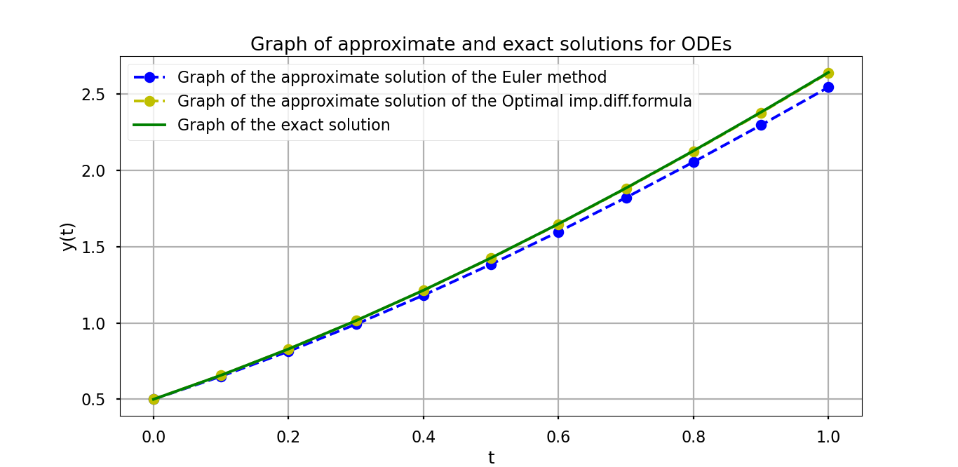
In this section, we give some numerical results in order to show tables and graphs of solutions and errors of our optimal explicit difference formulas (2.24) and optimal implicit difference formulas (3.18), with coefficients given correspondingly in Theorem 2.3 and Theorem 3.1.
We show the results of the created formulas in some examples in the form of tables and graphs. Here, of course, the results presented in the table are then shown in the graph.We have taken examples from the book by Burden R.L. et al [1] to illustrate numerical results.


In accordance with the table above, shown in Figures 1,3,5, on the left side of these Figures 2,4,6, graphs of approximate and exact solutions are shown, and on the right side of these Figures 2,4,6, graphs of the difference between the actual and approximate solutions. As can be seen from the results presented above, in a certain sense, optimal explicit formula give better results than the classical Euler formula.


In accordance with the table above, shown in Figure 7, on the left side of these Figure 8, graphs of approximate and exact solutions are shown, and on the right side of these Figure 8, graphs of the difference between the exact and approximate solutions. As can be seen from the result presented above, in a certain sense, optimal implicit difference formulas give better results than the classical Euler formula.
7. Conclusion
In conclusion, In this paper, new Adams-type optimal difference formulas are constructed and exact expressions for the exact estimation of their error are obtained. Moreover, we have shown that the results obtained by the optimal explicit difference formulas constructed in the Hilbert space are better than the results obtained by the Euler formula. In addition, the optimal implicit formula is more accurate than the optimal explicit formula and the effectiveness of the new optimal difference formulas was shown in the numerical results.
References
- [1] Burden R.L., Faires D.J., Burden A.M. Numerical Analysis. - Boston, MA : Cengage Learning, 2016, 896 p.
- [2] Ahmad Fadly Nurullah Rasedee, Mohammad Hasan Abdul Sathar, Siti Raihana Hamzah, Norizarina Ishak, Tze Jin Wong, Lee Feng Koo and Siti Nur Iqmal Ibrahim. Two-point block variable order step size multistep method for solving higher order ordinary differential equations directly. Journal of King Saud University - Science, vol.33, 2021, 101376, https://doi.org/10.1016/j.jksus.2021.101376
- [3] Adekoya Odunayo M. and Z.O. Ogunwobi. Comparison of Adams-Bashforth-Moulton Method and Milne-Simpson Method on Second Order Ordinary Differential Equation. Turkish Journal of Analysis and Number Theory, vol.9, no.1, 2021: 1-8., https://doi:10.12691/tjant-9-1-1.
- [4] N.S. Hoang, R.B. Sidje. On the equivalence of the continuous Adams-Bashforth method and Nordsiecks technique for changing the step size. Applied Mathematics Letters, 2013, 26, pp. 725-728.
- [5] Loïc Beuken, Olivier Cheffert, Aleksandra Tutueva, Denis Butusov and Vincent Legat. Numerical Stability and Performance of Semi-Explicit and Semi-Implicit Predictor-Corrector Methods. Mathematics, 2022, 10(12), https://doi.org/10.3390/math10122015
- [6] Aleksandra Tutueva and Denis Butusov. Stability Analysis and Optimization of Semi-Explicit Predictor-Corrector Methods. Mathematics, 2021, 9, 2463. https://doi.org/10.3390/math9192463
- [7] Babus̆ka I., Sobolev S.L. Optimization of numerical methods. - Apl. Mat., 1965, 10, 9-170.
- [8] Babus̆ka I., Vitasek E., Prager M. Numerical processes for solution of differential equations. - Mir, Moscow, 1969, 369 p.
- [9] Shadimetov Kh.M., Hayotov A.R. Optimal quadrature formulas in the sense of Sard in space. Calcolo, Springer, 2014, V.51, pp. 211-243.
- [10] Shadimetov Kh.M., Hayotov A.R. Construction of interpolation splines minimizing semi-norm in space. BIT Numer Math, Springer, 2013, V.53, pp. 545-563.
- [11] Shadimetov Kh.M. Functional statement of the problem of optimal difference formulas. Uzbek mathematical Journal, Tashkent, 2015, no.4, pp.179-183.
- [12] Shadimetov Kh.M., Mirzakabilov R.N. The problem on construction of difference formulas. Problems of Computational and Applied Mathematics, - Tashkent, 2018, no.5(17). pp. 95-101.
- [13] Sobolev S.L. Introduction to the theory of cubature formulas. - Nauka, Moscow, 1974, 808 p.
- [14] Sobolev S.L., Vaskevich V.L. Cubature fromulas. - Novosibirsk, 1996, 484 p.
- [15] Shadimetov Kh.M., Mirzakabilov R.N. On a construction method of optimal difference formulas. AIP Conference Proceedings, 2365, 020032, 2021.
- [16] Akhmedov D.M., Hayotov A.R., Shadimetov Kh.M. Optimal quadrature formulas with derivatives for Cauchy type singular integrals. Applied Mathematics and Computation, Elsevier, 2018, V.317, pp. 150-159.
- [17] Boltaev N.D., Hayotov A.R., Shadimetov Kh.M. Construction of Optimal Quadrature Formula for Numerical Calculation of Fourier Coefficients in Sobolev space . American Journal of Numerical Analysis, 2016, v.4, no.1, pp. 1-7.
- [18] Hayotov A.R., Karimov R.S. Optimal difference formula in the Hilbert space . Problems of Computational and Applied Mathematics, - Tashkent, 5(35), 129-136, (2021).
- [19] Dahlquits G. Convergence and stability in the numerical integration of ordinary differential equations. -Math. Scand., 1956, v.4, pp. 33-52.
- [20] Dahlquits G. Stability and error bounds in the numerical integration of ordinary differential equations. - Trans. Roy. Inst. Technol. Stockholm, 1959.
- [21] Shadimetov Kh. M., Mirzakabilov R. N. Optimal Difference Formulas in the Sobolev Space. - Contemporary Mathematics. Fundamental Directions, 2022, Vol.68, No.1, 167-177.
- [22] Shadimetov Kh.M., Hayotov A.R. Construction of a discrete analogue of a differential operator Uzbek Matematical Journal, - Tashkent, 2004, no. 2, pp. 85-95.